Intrinsic Curvature in the X-ray Spectra of BL Lacertae Objects

Abstract

We report results from XMM-Newton observations of thirteen X-ray bright BL Lacertae objects, selected from the Einstein Slew Survey sample. The survey was designed to look for evidence of departures of the X-ray spectra from a simple power law shape (i.e., curvature and/or line features), and to find objects worthy of deeper study. Our data are generally well fit by power-law models, with three cases having hard ($\Gamma<2;dN/dE\propto E^{-\Gamma}$) spectra that indicate synchrotron peaks at $E\lower 2.15277pt\hbox{$\;\buildrel>\over{\sim}\;$}5$ keV. Previous data had suggested a presence of absorption features in the X-ray spectra of some BL Lacs. In contrast, none of these spectra show convincing examples of line features, either in absorption or emission, suggesting that such features are rare amongst BL Lacs, or, more likely, artifacts caused by instrumental effects. We find significant evidence for intrinsic curvature (steepening by $d\Gamma/d({\rm log}E)=0.4\pm 0.15$) in fourteen of the seventeen X-ray spectra. This cannot be explained satisfactorily via excess absorption, since the curvature is essentially constant from $0.5-6$ keV, an observation which is inconsistent with the modest amounts of absorption that would be required. We use the XMM-Newton Optical Monitor data with concurrent radio monitoring to derive broadband spectral energy distributions and peak frequency estimates. From these we examine models of synchrotron emission and model the spectral curvature we see as the result of episodic particle acceleration.

1. Introduction

Among all active galactic nuclei, BL Lacertae (BL Lac) objects are the most dominated by variable, non-thermal emissions. BL Lacs often vary on time scales of days to hours at frequencies from optical through the $\gamma$-rays (see Ulrich, Maraschi & Urry 1997 for a review). Their emissions are dominated by a broad, featureless continuum, believed to originate in a relativistic jet oriented very close to our line of sight (see Urry & Padovani 1995 for a review). This component is thought to be responsible for their variability as well as their high optical polarization (Jannuzi, Smith & Elston 1994) and radio core-dominance (Rector et al. 2000, Rector & Stocke 2001 and references therein). The spectral energy distributions (SEDs) of BL Lacs appear to be dominated by synchrotron emission at radio to ultraviolet energies (up to X-ray energies for X-ray selected objects) and inverse-Compton emission at higher energies.

Previous observations of the X-ray spectra of BL Lacs have yielded somewhat confusing results. Worrall & Wilkes (1990) compiled the first examination of a relatively large sample of BL Lacs with Einstein. They found power-law shapes, with a wide range of spectral indices. This was confirmed by observations with HEAO-1 (Sambruna et al. 1994), ROSAT (Perlman et al. 1996a, Urry et al. 1996, Sambruna et al. 1996), ASCA (Kubo et al. 1998) and BeppoSAX (Wolter et al. 1998; Beckmann et al. 2002; Padovani et al. 2001, 2004). Those observations also found a pattern of harder X-ray spectra in objects with spectral peaks in the infrared to optical (often called low-energy peaked BL Lacs, or LBLs) than in those with spectral peaks in the UV to X-rays (often called high-energy peaked BL Lacs, or HBLs). The correlation between peak frequency and spectral index is strong, but not monotonic (Padovani, Giommi & Fiore 1997, Lamer et al. 1996, Padovani et al. 2001). The explanation put forward most often for the complex nature of this relationship was that it was due to observing the intrinsically curved synchrotron and inverse-Compton spectral components, peaked at a variety of frequencies, over only a restricted energy range.

If indeed there is curvature in the X-ray spectra of BL Lacs, one might expect to see evidence of this when larger bandpasses are examined, particularly in bright objects where high signal-to-noise can be attained. Several authors have found evidence of such curvature (Inoue & Takahara 1996; Takahashi et al. 1996; Tavecchio et al. 1998; Massaro et al. 2004a, b; Giommi et al. 2002) among a significant fraction (up to 50%) of HBLs. However, those authors did not analyze in detail the alternative possibility of an additional absorbing column, as had been assumed by other workers (e.g., Perlman et al. 1996a, Urry et al. 1996, Kubo et al. 1998, Wolter et al. 1998, Beckmann et al. 2002, Padovani et al. 2001).

Another issue is whether line features are present in the X-ray spectra. Early Einstein grating data for PKS 2155$-$304 suggested a soft X-ray deficit (Canizares & Kruper 1984), as did later Einstein Solid State Spectrometer data for a few of the brightest objects (Urry, Mushotzky & Holt 1986; Madejski et al. 1991). Examination of ASCA and BBXRT spectra of some of the brightest BL Lacs indicated a similar soft X-ray deficit, requiring a recovery of the spectrum towards even lower energies, as inferred from ROSAT PSPC data (PKS 2155$-$304, Madejski et al. 1992; H1426+428, Sambruna et al. 1997; PKS 0548$-$322, Sambruna & Mushotzky 1998). These features were all explained by invoking X-ray absorption features at 0.5–0.8 keV. However, not all bright BL Lacs were found to require such features (e.g., Mrk 421, Guainazzi et al. 1999); nor were such features found in stacked ROSAT spectra of the fainter EMSS BL Lacs (Perlman et al. 1996a). This lack of consensus regarding the presence or lack of X-ray spectral curvature and line features motivated us to use XMM-Newton to obtain high signal to noise (S/N) spectra of a significant sample of X-ray bright BL Lac objects with a single instrument.

The paper is organized as follows. In §2, we describe the sample, observations and data reduction procedures. In §3 we give the results of our X-ray spectral fits, specifically concentrating on issues regarding spectral curvature and the presence or lack of spectral lines. In §4, we focus on models for X-ray spectral curvature and particle acceleration. Finally, in §5, we conclude with a summary and a discussion of the implications of our results.

2. Sample, Data and Data Reduction

2.1. Sample Design

Our targets were selected from the Einstein Slew Survey sample of BL Lacs (Perlman et al. 1996b). The Slew Survey is ideal for this purpose because it is a nearly all-sky survey, with mean limiting flux F (0.3–3.5 keV) $\sim 1.4\times 10^{-11}{\rm~{}erg~{}cm^{-2}~{}s^{-1}}$ (Elvis et al. 1992). Besides being the largest collection of BL Lacs at such high X-ray fluxes, the Slew Survey was the first sample to contain statistically significant numbers of both HBLs and LBLs. We used this property to design a sample of 36 objects, which are the X-ray brightest in the LBL and HBL sub-classes. Of these, 11 (nearly all HBLs) were on the XMM-Newton or Chandra observing lists of other projects and so we did not choose to observe them again. We were awarded observing time for the 12 X-ray brightest of the remaining 24 objects, which unfortunately include only the HBL subclass: LBLs were approved only in priority C and none were observed. under a separate proposal by some members of our team. Table 1 lists the objects we observed. We do not discuss here the objects observed by other workers, which have already appeared in the literature (e.g., Boller et al. 2001; Watson et al. 2004; Blustin, Page & Branduardi 2004; Cagnoni et al. 2004); however, where appropriate we make use of their results.

2.2. Instruments and Observations

We observed each object with all instruments aboard XMM-Newton. The XMM-Newton Observatory (Jansen et al. 2001) consists of three coaligned 7.5 m focal length X-ray telescopes, focussing X-rays onto the European Photon Imaging Camera (EPIC) and two Reflection Grating Spectrometers (RGS1 and RGS2 respectively). The EPIC has three detectors, sensitive in the 0.3-10 keV band: two metal-oxide-semiconductor (MOS) and one p-n junction (PN) CCD arrays. These instruments provide moderate-resolution X-ray imaging (PSF FWHM $6^{\prime\prime}$) and spectroscopy ($E/\delta E\approx 20-50$, depending on energy). The two RGS instruments provide spectroscopy at higher resolution, with $E/\delta E\approx 300$.

Because the main goal was to address the sample properties of the BL Lac class, rather than to obtain very deep observations of individual objects, our integration times were short, $\sim 5$ ks on each instrument. Table 1 lists the EPIC PN and MOS good on-source times and count rates. Figure 1 shows two examples of our EPIC observations, fit with a single-power-law model (§3). As can be seen, the S/N of the EPIC data were quite high (20-50 below 1 keV; lower at high energies). The RGS spectra (§3.3) had much more modest S/N, due to the lower effective area of the gratings. In all but one observation, the EPIC was used in small-window mode in order to minimize the effects of pileup. On most objects, the THIN filter was used in both the PN and MOS; however, for the brighter objects we used the MEDIUM filter to avoid contamination from optical light due to the object (none of the targets has other X-ray bright objects within the field).

Eight XMM-Newton observations were significantly affected by proton flares. Of these, six were impacted badly enough that one or more of the X-ray instruments had to be shut off because of the high background, and in two, all instruments were shut off during the observation. For the six observations where X-ray instruments were shut off completely due to high background, the observation was automatically attempted again (see Table 1 for details). As a result, four objects were observed twice and one object was observed three times. We inspected all data from XMM-Newton, regardless of whether the observation was affected by flares. We generally found that even for the observations impacted by proton flaring, some of the X-ray data were usable as long as the instruments were not shut off.

XMM-Newton also has a coaligned 30 cm optical/UV telescope, the Optical Monitor (OM). The OM is sensitive between $\lambda=1000-6000$ Å and has a typical angular resolution of $\sim 2^{\prime\prime}$. OM data were gathered for all objects, but in only one band due to observing restrictions in AO1 that did not allow multi-band observations within $\lesssim$ 2 hours. All but one OM dataset was gathered using the UVW2 filter, which is sensitive between $2000-3000$ Å. Data were taken in exposures of 800 s in order to allow for the possibility of finding short-timescale optical variability, but no such variations were found. We include in Table 2 the near-UV magnitude of each source, as derived from the OM data.

We also monitored the radio fluxes of all but one of these objects using the University of Michigan Radio Observatory (UMRAO) 26-m telescope (Aller et al. 1985). We observed each object at one or more of three frequencies: 4.5, 8.0 and 14.5 GHz, but some were below its sensitivity limitations (typically 50 mJy at 8.0 GHz). These data are also given in Table 2; two example datasets are shown in Figure 2.

2.3. Data Reduction Procedures

All source and background extraction, as well as examination of the lightcurves, was done in the XMM-Newton Science Analysis System (SAS) v5.4.1. We performed a standard reduction of the events list for the PN, MOS and RGS data, which involves the subtraction of hot and dead pixels, removal of events due to electronic noise, and the correction of event energies for charge transfer losses. The PN files were also filtered to include only single, double, and single+double events (PATTERN $\leq$ 4) while the MOS included all single to quadruple events (PATTERN $\leq$ 12). Photons were extracted in all instruments using a $45^{\prime\prime}$ aperture (which, for the PN and MOS, was circular in shape). In cases where pile-up was significant, an annular extraction region was used to filter out the pixels affected most severely.

We extracted lightcurves for every dataset, and filtered out all high-background time intervals. To do so, we determined the count rate in the 10 – 15 keV band for the entire PN and MOS detectors. Since the source count rate in this band is quite small, intervals with more than 0.3 ct s^-1 for the PN and 1.5 ct s^-1 for MOS were rejected. Once this was done, the datasets were searched for evidence of source variability on $<5$ ks timescales (using the nominal 0.3 – 10 keV band); no such variability was found during any of these observations. Spectra were extracted, as discussed in the next section. These spectra were limited to the energy range 0.2–10 keV for the MOS and 0.15–15 keV for the PN; however, for the detailed spectral fits, we used a more restricted energy range, as given below, to account for possible residual calibration uncertainties (see Andersson & Madejski 2004 for detailed discsusion).

For the MOS data, the background region used was the same size as the source region in a place where there are no visible sources (typically off axis). For the PN data, the background region was once again the same size as the source region at a point where the RAWY values were the same as the source. Because of the high fluxes of these sources and the use of the small-window mode (as well as the relatively stringent criteria to reject data segments affected by flares), we did not extract background maps (see e.g., Read & Ponman 2003; note that the background maps vary little within the portion of the detectors used for small-window mode). It should, however, be noted that because of the use of the small-window mode the background regions are of necessity close to the source itself, and thus it is possible that some small amount of source flux could be subtracted. This effect causes mainly a small error in the absolute flux of the sources, and thus does not affect our analysis of possible curvature or line features. We did, however, attempt to minimize this effect by placing the background region as far away from the source as possible within the small window.

For the OM data, we performed simple aperture photometry, with a $6^{\prime\prime}$ circular aperture, using an annulus for background subtraction. The size of the annulus was typically $20^{\prime\prime}$; however, in the case of a few objects, a nearby companion necessitated some adjustment. We then used the zero-points published in the XMM-Newton Observer’s Handbook (Issue 2.1) to calculate absolute optical fluxes. The UMRAO data were reduced according to the procedure outlined in Aller et al. (1985). The fluxes and magnitudes from UMRAO and the OM at the time of observation are summarized in Table 2.

3. X-ray Spectral Fits

As the sources were well centered in the XMM observing region, we used standard response (RMF) matrices, picking the one closest in time to each observation. The Ancillary Response Files (ARFs) were generated using the arfgen function of SAS 5.4.1. To assure the validity of Gaussian statistics, we grouped the data, combining the instrumental channels such that each new bin would have at least 40 counts. The exceptions are 1ES 0145+138 (OBSID 0094383401) and 1ES 1255+244 (OBSID 0094383201), where because of the small number of counts we rebinned to 10 counts/bin for the MOS data and 15 counts/bin for the PN data. All the PN data were fit in the 1.1–10.0 keV range, while all the MOS data were fit in the 0.3–10.0 keV range, except for those of the faintest objects which we capped at 7.0 keV due to low count rates at the highest energies.

All X-ray spectral modeling was done in XSPEC v11.0. Continuum models were fit only to the PN and MOS data and then applied to the RGS data. We used both the EPIC and RGS data to search for absorption and/or emission lines (§3.3). The PN and MOS data were fit simultaneously as well as individually in order to spot any calibration problems and/or instrument specific problems that might have occurred during the observation. Where multiple observations of an object were obtained (Table 1, §2.2), each observation was reduced and analyzed separately, as we expected that the flux and X-ray spectrum would change between those observations, as was indeed the case.

3.1. Spectral Modeling in the broad X-ray band

Initially, two models were fit to each EPIC spectrum:

1. A single power law,

$dN/dE=ke^{-\sigma(E)N_{H,Gal}}e^{-\sigma(E)N_{H,int}(1+z)}~{}E^{-\Gamma}$.

2. A logarithmic parabola,

$dN/dE=ke^{-\sigma(E)N_{H,Gal}}e^{-\sigma(E)N_{H,int}(1+z)}~{}E^{(-\Gamma+\beta Log(E))}$.

In each case, we attempted fits with two different treatments of the absorbing column: with $N_{H,int}=0$ and with $N_{H,int}$ (assumed to be at the redshift of the source) allowed to vary freely. We took values of $N_{H,Gal}$ from Stark et al. (1992), although it is probable that the actual Galactic absorbing column for each object might be slightly different due to the low resolution of the Stark et al. survey. In all cases, the opacity associated with the intervening column density was modeled by a standard Morrison & McCammonn (1983) absorption model. The motivation to try both the power law model, as well as the less-used logarithmic parabola model (described in Giommi et al. 2002 and references therein), was that both simple power-law and continuously curving spectral shapes can reasonably be expected depending on the model adopted for synchrotron aging and acceleration (Leahy 1991, Massaro 2002). Our spectral fits for the single power-law model are summarized in Table 3. In Figure 1, we show as examples spectra of two objects fit with the single power-law model.

As can be seen, the spectral indices we found range from $\Gamma=1.7-2.9$ (corresponding to energy spectral indices $\alpha=0.7-1.9$), with twelve of seventeen being in the range $\Gamma=2.1-2.7$. These spectral indices are similar to the findings of past observations of HBLs by ROSAT (Perlman al. 1996a, Padovani et al. 1997), ASCA (Kubo et al. 1998) and BeppoSAX (Wolter et al. 1998, Beckmann et al. 2001). Three spectra were found to be flat ($\Gamma<2$). These objects are likely to have synchrotron peaks at energies higher than $\sim 5$ keV (see also §4).

In the three objects where repeated observations were made, we see significant variability both in flux and spectral shape (Table 3). In all of those objects, the highest flux state observed also has the hardest spectrum, in agreement with the known spectral variability properties of BL Lac objects (e.g., Ulrich et al. 1997 and references therein). However, the correlation between a harder spectrum and higher X-ray flux is not one-to-one, as indicated by the three observations of 1ES1959+650.

3.2. X-ray Spectral Curvature

In fourteen of seventeen observations, a better fit (significant at the $>99$% level according to $F$-test results; see Table 3) was obtained by allowing for the possibility of spectral curvature (over and above the default, power-law plus Galactic $N_{H}$ model). This curvature can either be intrinsic, or the result of additional absorption due to material either within the BL Lac’s host galaxy or our own. As indicated above, we first investigated the possibility that additional absorption was present; the result of these procedures is given in Table 3. As can be seen, in 13 of 14 observations the column required is $\lower 2.15277pt\hbox{$\;\buildrel>\over{\sim}\;$}20$% of the Galactic figure. We also investigated the alternate possibility of intrinsic curvature, using the logarithmic parabola model as well as an alternate model, detailed later, where we simply fitted power-laws independently in four sub-bands, and obtained results of similar significance. The results of this procedure are given in Table 4 and discussed below. Importantly, it is impossible to discriminate a priori between the two models due to their similar mathematical forms (see above). It is, however, possible to use other information and perform other tests.

We first inspected the implied columns to check the reasonability of the idea that the spectral curvature was the result of additional absorbing material. We believe that additional absorbing material is less likely for three reasons. First, the typical BL Lac’s host galaxy is a bright elliptical, where columns this high would not normally be expected except in extreme cases (Goudfrooij et al. 1994). Also, in 1ES1959+650, one of the three objects where repeated observations were done, the implied $N_{H}$ appears to vary between epochs. This requires the absorbing material to have been in a region smaller than $\sim 1$ light-month in size. This would imply densities $n\lower 2.15277pt\hbox{$\;\buildrel>\over{\sim}\;$}10^{3}-10^{4}{\rm~{}cm^{-3}}$, which is outwardly not unreasonable for the inner regions of the AGN. But the implied density would have to climb with decreasing timescale, as $\tau^{-3/2}$, meaning that unreasonable column densities would be reached if $N_{H}$ appeared to vary on timescales only 1-2 orders of magnitude smaller, which are not uncommon for flux variability among BL Lacs (Ulrich et al. 1997). Finally, there is no indication from optical or UV spectroscopy that BL Lac objects would have any significant neutral material in the line of sight to the nucleus (e.g., Perlman et al. 1996; Rector et al. 2000; Rector & Stocke 2001; Kinney et al. 1991; Lanzetta, Turnshek & Sandoval 1993; Penton & Shull 1996). This material, in principle, can be partially ionized, providing no opacity in the optical and UV, but absorbing via individual edges in the soft X-ray band. This can be ruled out as a general property on the basis of an absence of any individual spectral features in the RGS data (§3.3), although we cannot exclude it in the spectra of fainter objects.

This is persuasive but not conclusive evidence that these spectra have intrinsic X-ray spectral curvature. To test this idea further, we split the XMM-Newton data into four sub-bands: 0.5–1 keV, 1–2 keV, 2–4 keV and 4–10 keV, and fit each sub-band individually with a power-law model. For this exercise we assumed an $N_{H}$ value fixed at Galactic, and used the MOS data only below 2 keV and both the PN and MOS data at higher energies. This was done because of the known issues in cross-calibrating PN data with those from the MOS at lower energies, especially near 1 keV (see also the first paragraph of §3, above). The results of this procedure are given in Table 4, and four examples of these fits are shown in Figure 3. We note that the overall $\chi^{2}$ values for these fits are comparable to those achieved by varying $N_{H}$; however it is impossible to use an $F$-test to compare them because of the differing ways in which data was selected for this procedure. As can be seen, the typical X-ray curvature seen in our sample is nearly constant, even up to the highest energy band. We have characterized this curvature by looking at the $d\Gamma/d(\log E)$ for each object. This information is included in Table 4. As can be seen, our data are consistent with a $\langle d\Gamma/d(\log E)\rangle\approx 0.4\pm 0.15$ in fourteen of seventeen observations (the same ones for which spectral curvature was indicated as mentioned above). This is not consistent with the observed columns in these objects, which range from $3-20\times 10^{20}{\rm~{}cm^{-2}}$. At such moderate columns, it is typical for the spectrum above about 1 keV to be relatively insensitive to the absorbing column. This is yet another argument (albeit indirect) against the presence of additional absorbing material explaining the observed spectral curvature in these objects.

As already noted, we also attempted to model intrinsic curvature by fitting a logarithmic parabola form. The information for these fits is also given in Table 4. The logarithmic parabola is characterized by both a spectral index and a curvature parameter, $\beta$. The spectral form is somewhat different mathematically from either of the other forms; however, it is essentially similar to the application of a constant $d\Gamma/d(\log E)$, with the added advantage of allowing a consistent fit in the entire band. In theory, the value of the curvature parameter $\beta$ should be equivalent to the value of $\langle d\Gamma/d(\log E)\rangle$ found using several sub-bands. Inspection of Table 4 shows that these are indeed similar, albeit with small variations in each case. The mean curvature required for the objects where this is indicated by the $F$-tests is essentially identical, in fact: $\langle\beta\rangle=0.37$ versus $\langle d/\Gamma/d(\log E)\rangle=0.38$.

Giommi et al. (2002) also found good evidence for intrinsic X-ray spectral curvature (which they modeled by the same logarithmic parabola form) in about half of the HBLs observed by BeppoSAX. The value of $\langle\beta\rangle$ they found is consistent with our findings. However, the proportion of curved spectra in Giommi et al. (2002) is considerably lower than we see. The difference cannot be explained by our small sample, as twelve of thirteen objects observed by BeppoSAX were also observed by us with XMM-Newton, and of those, for six the best representation of their BeppoSAX spectrum was a logarithmic parabola plus fixed absorption (although n.b., Giommi et al. 2002 did not fit a variable absorption model for any object). We believe it is much more likely that the reason for the larger fraction found here lies in the higher signal to noise and resolution of these spectra compared to those from BeppoSAX. This is supported by the fact that if one examines the variable $N_{H}$ fits, the 6 objects where Giommi et al. (2002) required a logarithmic parabola are best fitted by significantly higher absorbing columns than those which Giommi et al. (2002) was able to fit adequately with a single power law.

Our conclusion from the above is that we believe the most appropriate model for the spectral curvature we see is intrinsic, rather than due to additional absorption. Given the similar values of $\chi^{2}$, our primary motivation for concluding this is the indirect lines of evidence presented above regarding the implausibility of additional absorbing columns under these circumstances. We will proceed on this basis in the upcoming discussion.

To close this discussion of intrinsically curved spectra, it is useful to compare the fits and shape of the spectrum achieved for a given object under a simple power law model (with Galactic $N_{H}$) with those implied by the logarithmic power law form. We show this comparison in Figure 4, for one of the spectra of 1ES1959+650, specifically OBSID 0094383301. There comparison is shown in two forms: at top, we show the comparison in terms of the detected spectrum (folded into the instrumental response), while at bottom it is shown in terms of emitted energy. The plots at top enable us to see the real differences in the quality of the fit: the simple power law model (Figure 4, top left) clearly overpredicts the observed spectrum at $E>1$ keV, and slightly underpredicts the lower-noise MOS data at 1-1.5 keV. But at higher energies it is the PN data which have the greater ability to distinguish between the two models, and the simple power law model overpredicts the data at energies higher than about 5 keV. As can be seen, the logarithmic power law model (Figure 4, top right) fits the data much better. The plots at bottom enable us to see the form of the curvature: note that above $\sim 1$ keV essentially no curvature would be seen, if the spectrum followed a simple power law model (Figure 4, bottom left). However, under the logarithmic parabola model (Figure 4, bottom right), we see that there is in fact significant curvature seen at higher energies, albeit of a mild, gradual form. This is presumably why this curvature was not seen by earlier satellites, which suffered from either a much smaller spectral range (for all satellites except BeppoSAX) and/or much lower signal to noise (all other satellites).

3.3. Spectral Line Features in BL Lacs?

We inspected each spectrum thoroughly for spectral features. We did not find convincing evidence for line features in any of these spectra. To quantify this, both the EPIC and RGS data for the 12 highest signal-to-noise spectra were searched for absorption features in XSPEC (we did not search datasets where either instruments were turned off and/or the statistics were inadequate). The best-fit broadband model (Table 4) was used as the seed model in each case, and the RGS data were grouped in bins with a minimum of 20 photons apiece (following our practice for the EPIC data; §3.1). We then artificially set a line feature of 5 eV physical width, and covering fraction of 0.5, and then stepped it through the range 0.5 to 4.5 keV in increments of 0.01 keV using STEPPAR, and assessed the significance of features using the $\Delta\chi^{2}$ (A $3\sigma$ feature has $\Delta\chi^{2}=-9.21$, while a $4\sigma$ feature has $\Delta\chi^{2}=-18.42$). Higher energies were not searched due to the small effective area and poor statistics. Once features were found, we then fixed the energy and allowed XSPEC to converge on a best-fit width. This procedure found six narrow features, as shown in Table 5, in four of the datasets, but in most (1ES 0120+340 OBSID 0094382101, 1ES0323 OBSID 0094382501, 1ES 0414+009 OBSID 0094383101, 1ES0647+250 OBSID 0094380901, 1ES1133+704 OBSID0094170101, 1ES1255+244 OBSID 0094383001, 1ES 1553+113 OBSID 0094380801, 1ES1959+650 OBSID 0094383501), no features were found.

Are these features real? As can be seen, all but one are between 3-4 $\sigma$, with one barely over 4$\sigma$. For Gaussian statistics, $P(3\sigma)=0.0027$, while $P(4\sigma)=0.000318$. As can be seen from Table 3, the typical EPIC dataset in our sample is $\sim 300$ channels, as is the typical RGS dataset (n.b., the number of channels is not significantly greater due to the relatively poor statistics resulting from the short exposure times). Thus the result of 5 features at $\lower 2.15277pt\hbox{$\;\buildrel>\over{\sim}\;$}3\sigma$ and 1 feature at $>4\sigma$ in $\sim 3600$ spectral channels is consistent with what one would expect from statistical noise (respectively $10\pm 3$ features at $>3\sigma$ and $1\pm 1$ feature at $>4\sigma$). Moreover, as noted in Table 5, none of the features found in any of the spectra are present in the spectra from all the EPIC and RGS instruments. Thus, we believe all are the result of random noise and therefore not real spectral lines. The limits shown in Table 5 can be taken as representative of the detection limits of our data, which range from $\sim 5$ up to $\sim 50$ eV depending on count rate.

This conclusion differs from findings based on data from earlier instruments. We are confident of our result based on the relatively high signal-to-noise of the XMM-Newton spectra. We note, however, that narrow, small equivalent width absorption lines such as those inferred (at intermediate redshifts) from Chandra grating observations of BL Lac objects by Nicastro et al. (2002; see also Cagnoni et al. 2004), or those due to ionized oxygen in the hot halo of our Galaxy (e.g., Nicastro et al. 2002, McKernan, Yaqoob & Reynolds 2004), are not excluded by the data in-hand. The determination of presence or absence of such features require much higher S/N data than are available in our sample.

It is worth noting that a similar absence of strong spectral features was also found in another, independent study of the XMM-Newton X-ray spectra of four of the five BL Lacs where BBXRT and ASCA spectra appeared to show these line features, specifically H1219+301, Mkn 501, H1426+428 and H0548-322 (Blustin et al. 2004). Those authors reported that if any of the previously found absorption features were indeed real, they had to represent a transient phenomenon. They found this particular conclusion unlikely, ruling it out at 93% confidence based on the assumption that the (multiple) XMM-Newton observations of those objects represented random time instances. The objects in the Blustin et al. (2004) sample are not discussed here, and moreover, our integration times are smaller so we have used primarily the EPIC data and not the RGS. However, our results are in the same vein. With the addition of our data, it appears unlikely that the absorption features found with ASCA and BBXRT were transient phenomena.

The most likely explanation of the previously reported line features is a combination of mis-calibration of the previous instruments and the use of overly simplistic spectral models. As an example, a deficit of low energy counts in the ASCA data has been previously noted in reference to the data for NGC 5548 (Iwasawa, Fabian, and Nandra 1999); the simultaneous ASCA and ROSAT PSPC observation implied significantly higher flux below 0.5 keV than any reasonable spectral extrapolation of the ASCA SIS data would allow. Another reason is that a spectral curvature of exactly the type discussed in this paper would, at low resolution and lower signal-to-noise, mimic an absorption feature when the underlying spectrum was assumed to be a simple power law. However, the confirmation that an absorption feature was measured would require data below the energy of such a putative feature, and such data were not always available (as was the case for the Einstein SSS as well as SSS + MPC data). We therefore suggest that the claims made by earlier workers were a byproduct of the particular simple power law model used, while the effect was due to gradual spectral curvature and/or instrumental effects rather than absorption features from material along the line of sight.

4. Modeling the X-ray and Broadband Spectral Characteristics

We have constructed broadband spectral energy distributions (SEDs) for each object using the EPIC data, in conjunction with the data from the OM and the UMRAO flux nearest in time to the XMM observation. For objects which were too faint in either the optical or radio at the time of observation to register a positive detection on either the OM or UMRAO, we have used POSS plates to obtain an average optical flux and radio fluxes from the literature (Perlman et al. 1996b and sources therein) for the SED. We fit to these data a simple parabolic model, in order to obtain a peak frequency, $\nu_{peak}$. We did not assume a standard synchrotron spectrum for this procedure because the small amount of data we have do not adequately constrain these models (see e.g., Leahy 1991, Pacholczyk 1970). For a few objects, where the initial fit was not good, we had to modify a single non-simultaneous point to find a convincing value of $\nu_{peak}$.

In Table 6 we summarize the broadband spectral data and $\nu_{peak}$ for every object in our sample. As can be seen, our objects range between log $\nu_{peak}\approx 14.5-18$, as expected for HBL-type and intermediate objects. A few objects, noted in Table 6, have very flat X-ray spectral index and/or significant evidence of $\nu_{peak}>10^{18}$ Hz. Our procedure yielded $\nu_{peak}$ values considerably in excess of $10^{18}$ Hz for all these objects (see also §3.1), but in Table 6 we list them as having $\nu_{peak}=10^{18}$ Hz because our data are not able to test for a higher peak frequency given their frequency space coverage.

We then proceeded to test for correlations between broadband spectral properties and both $\Gamma$ and $d\Gamma/d(logE)$. We then tested each for correlations using standard statistical tests (Spearman’s rank correlation, $\rho$, and Pearson’s correlation coefficient, $r$). These plots and their physical implications are the main subject of this section.

In Figure 5 we show plots of $\Gamma$ versus $\alpha_{ro}$ (left), $\alpha_{ox}$ (middle) and $\nu_{peak}$. As can be seen, our data show significant anti-correlations between $\Gamma$ and $\nu_{peak}$ ($r=-0.741,\rho=-0.781,P=0.18$%) and between $\Gamma$ and $\alpha_{ox}$ ($r=0.609,\rho=0.634,P=1.1$%) but no significant correlation between $\Gamma$ and and $\alpha_{ro}$ ($r=0.036,\rho=-0.05,P=84.0$%). This constellation of results is consistent with the $\alpha_{x}$ – $\nu_{peak}$ relation of Padovani et al. (1997), when one considers that the range of $\nu_{peak}$ values we cover is only $\sim 3$ decades.

4.1. Statistical Particle Acceleration?

The observed spectra exhibit curvature over a frequency range from $0.5$ keV to $10$ keV, in the sense of a gradual steepening with increasing energy. Assuming that the observed emission is synchrotron radiation, this implies that the electron distribution responsible for this emission is not the typical power law predicted by particle acceleration schemes (for a recent review see Gallant 2002). Instead, the electron spectrum has to gradually curve downwards in a way that produces the observed spectra. Given that X-ray synchrotron emission requires in situ particle acceleration due to the short radiative lifetimes of the emitting particles ($\tau_{sync}=1.2\times 10^{3}B^{-3/2}_{G}E_{\rm keV}^{-1/2}\delta^{-1/2}$ s; Rybicki & Lightman 1979), the ultimate physics behind curved X-ray spectra must be connected on a very basic level with the nature of particle acceleration in these systems. Here and in the next subsection we discuss possible solutions to this problem.

In Massaro et al. (2004b) a log-parabolic spectral curvature was fit to the X-ray spectrum and broadband SED of Mkn 421 in several flux states. Those authors modeled the log-parabolic curvature via a statistical particle acceleration process under which a particle $i$ with energy $\gamma_{i}$ in a given region has a finite probability ($<1$) of being accelerated, where the probability is given by $p_{i}=g/\gamma_{i}^{q}$, where $g,q$ are positive constants. They show in their paper that this leads analytically to a log-parabolic curvature form (see their §6 and equations (10)-(18)), and predicts a linear correlation between the X-ray spectral index, $\Gamma_{x}$, and $d\Gamma/d(logE)$. In Figure 6, we show plots of $\nu_{peak}$ versus $d\Gamma/d(logE)$ (top) as well as $\Gamma_{x}$ versus $d\Gamma/d(logE)$ (bottom). As can be seen, neither of these plots shows a significant correlation ($\nu_{peak}$ versus $d\Gamma/d(logE):r=0.615,\rho=0.393,P=11.6$% ; $\Gamma_{x}$ versus $d\Gamma/d(logE):r=-0.24,\rho=0.014,P=95.3$%). The results are similar for tests of $\nu_{peak}$ and $\Gamma$ versus $\beta$. Thus our data do not support the model of Massaro et al. (2004b). One possible reason why this is so is that Massaro et al. (2004b) model particle acceleration only, and do not include losses. Moreover, the statistical particle acceleration is still assumed to be time-invariant at all locations in the jet and hence the issue of variability is not addressed.

4.2. Spectral Curvature: a Signature of Episodic Particle Acceleration?

The results of §4.1 prompt us to look for another explanation that takes into account the known observational properties of jets and particularly blazars. Another motivation for this is the recent result of Perlman & Wilson (2005) that standard, continuous injection models of particle acceleration consistently overpredict the X-ray flux of the M87 jet by large factors (up to $\sim 100$ at 1 keV, varying with energy roughly as $E^{0.4}$). The interpretation advanced in that paper was one of a position- and energy-variable (but not time-variable) filling factor for particle acceleration. The Perlman & Wilson work, however, does not explore the issue of spectral curvature, as the statistics in most components of the M87 jet are inadequate for this purpose; nor does it explore issues related to variability, which are known to be of paramount importance for BL Lac objects.

In this subsection we address these issues directly, by demonstrating that curved electron particle spectra can be produced if the particle acceleration is episodic. Importantly, this model assumes only a time-variable particle acceleration which in an integrated sense should be indistinguishable from a a spatial average. Unlike the case of M87, here we have no spatial information regarding the distribution of jet X-ray emission and/or particle acceleration. Instead, we know that variability is an important characteristic of blazar jets and thus we optimize our model for this case. We explore these subjects more deeply in a later paper (Georganopoulos & Perlman, in preparation) that fully outlines a model considered in brief form below.

Consider a zone, possibly a shock, where electrons with Lorentz factor $\gamma_{0}$ are injected at a rate of $Q$ electrons per second and accelerated to higher energies. Following Kirk, Rieger, & Mastichiadis (1998), the kinetic equation describing particle acceleration is

$${\partial n\over\partial t}={\partial\over\partial\gamma}\left[\left({\gamma\over t_{acc}}-\beta\gamma^{2}\right)n\right]+{n\over t_{esc}}=Q\delta(\gamma-\gamma_{0}),$$ (1)

where $n(\gamma,t)$ is the electron energy distribution, $1/t_{acc}$ is the particle acceleration rate, $1/t_{esc}$ is the escape rate of particles from the acceleration region, and

$$\beta={3\over 4}{\sigma_{T}\over m_{e}c}U$$ (2)

with $\sigma_{T}$ the Thomson cross-section and U the total energy density of the magnetic field and ambient photons. Assuming that the injection started at time $t=0$, the electron energy distribution after time $t$ will be a power law with electron index $s=1+t_{acc}/t_{esc}$ up to a Lorentz factor

$$\gamma_{1}(t)=\left({1\over\gamma_{max}}+\left[{1\over\gamma_{0}}-{1\over\gamma_{max}}\right]e^{-t/t_{acc}}\right)^{-1},$$ (3)

where $\gamma_{max}=1/\beta t_{acc}$ is the maximum energy electrons reach asymptotically if the particle acceleration mechanism operates for $t\gg\ln[(\gamma_{max}-\gamma_{0})/\gamma_{0}]t_{acc}$. The time $t$ required for electrons to be accelerated up to Lorentz factor $\gamma_{1}$ is

$$t(\gamma_{1})=t_{acc}\ln{\gamma_{1}(\gamma_{max}-\gamma_{0})\over\gamma_{0}(\gamma_{max}-\gamma_{1})}.$$ (4)

If we assume that particle acceleration is characterized by a typical timescale $T$, then the electron distribution at any time $0\leq t\leq T$ is a power law that cuts off at a Lorentz factor $\gamma(t)$, reaching its maximum Lorentz factor $\gamma_{1}(T)$ at $t=T$. Particle acceleration ceases to operate at $t=T$, and the total time $\tau$ over which electrons of Lorentz factor $\gamma$ are provided by the particle acceleration mechanism is

$$\tau=T-t=t_{acc}\ln{\gamma_{1}(\gamma_{max}-\gamma)\over\gamma(\gamma_{max}-\gamma_{1})}.$$ (5)

The time $\tau$ is also the time during which an electron of Lorentz factor $\gamma$ radiates, as long as the radiative cooling timescale $t_{rad}=1/\beta\gamma=t_{acc}\gamma_{max}/\gamma$ satisfies the condition $t_{rad}\ll\tau$. In other words, $\tau$ is the total time the accelerated electron distribution is non-zero at electron Lorentz factor $\gamma$; note that, as is apparent from Eq. (5), the condition $t_{rad}\ll\tau$ can always be satisfied for $\gamma_{1}$ sufficiently close to $\gamma_{max}$. If the light crossing time of the emission region or the integration time of our observations is greater than $T$, then we effectively observe a time averaged electron distribution $\langle n(\gamma)\rangle$ which is the product of a power law multiplied by a logarithmic term representing the time interval this power law is available at each energy:

$$\langle n(\gamma)\rangle\propto\gamma^{-s}\ln{\gamma_{1}(\gamma_{max}-\gamma)\over\gamma(\gamma_{max}-\gamma_{1})},\;\gamma\leq\gamma_{1}.$$ (6)

Using the the $\delta$-function approximation (i.e., an electron of Lorentz factor $\gamma$ produces synchrotron photons only at the critical synchrotron energy) to calculate the synchrotron emission, we obtain an observed photon spectrum

$${dN\over dE}\propto E^{-(s+1)/2}\ln{E_{1}^{1/2}(E_{max}^{1/2}-E^{1/2})\over E^{1/2}(E_{max}^{1/2}-E_{1}^{1/2})},\;E\leq E_{1},$$ (7)

where $E_{1}$ and $E_{max}$ are the synchrotron energies produced by electrons of Lorentz factor $\gamma_{1}$ and $\gamma_{max}$ respectively. In Figure 7 we show the photon spectrum and photon index as a function of energy, for the following parameter choices: $s=3.0,E_{max}=100$ keV and $E_{1}=50$keV. As can be seen, the spectrum steepens gradually, with $\Gamma$ increasing at a fairly constant rate up to $\sim$ few keV, and then dramatically at $E\gtrsim 10$ KeV. If our interpretation of the steepening is correct, we expect to see an increasing curvature in future observations above the $10$ keV upper limit of XMM-Newton, as predicted in equation (7) (see Figure 7). One might also expect that in other objects, e.g., LBL, this cutoff might occur at lower energies. In LBL, however, we do not observe such steep values of $\Gamma$, but rather, flat X-ray spectra are seen ($\Gamma<2$; see Padovani et al. 2001, 2004), which are typically interpreted as being dominated by inverse-Comtpon emission (Padovani et al. 1997, Lamer et al. 1996). In practice, it may be difficult to observe this steepening because as the curvature of the synchrotron component increases, the spectrum is essentially cutting off and at some point the observed spectrum will begin to be dominated by the onset of the Compton component. What one might expect to see in practice, then, would be concave spectra (i.e., increasing $\Gamma$) up until the two components cross, with an inflection point at their crossing point and then a constant value of $\Gamma$ ($<2$) at higher energies. One final thing that should be noted here is that above 10 keV, almost all the HBL spectra that currently exist are for objects that are currently in a flaring state, where we would not expect to see significant steepening because the particle acceleration is still at or near its maximum. Also, there are no currently available instruments that would be sufficiently sensitive at $E>10$ keV to search for further steepening in the spectrum of HBLs.

The two energies $E_{1}$ and $E_{max}$ appearing in Equation (7) can be derived through spectral fitting. However, their values alone are offering little insight to the physical conditions in the source, because they depend on a series of parameters ($B$, $t_{acc}$, $\gamma_{0}$, $T$). As we discuss in §5, additional information from frequency-dependent variability can be used to constrain the physical state of the source.

5. Conclusions

We have presented 17 high-signal-to-noise XMM-Newton X-ray spectra for 13 BL Lac objects. These spectra do not show any spectral lines, contrary to expectations from some previous observations. We believe the reason for this discrepancy is due to a combination of overly simplistic spectral models and/or insufficiently precise calibration of previous instruments. As a result the intrinsic X-ray spectra of BL Lac objects appear to be quite featureless, giving no sign as to the physics of any region within the central engine, other than the jet itself. This is quite different from all other non-blazar type sources, where some line features, in either emission or absorption, are seen. This can be interpreted in the context of unified scheme models (e.g., Urry & Padovani 1995), under which the jet emission is Doppler boosted because it is seen at small angles to our line of sight. It is, however, difficult to address the issue of the necessary viewing angles to produce the degree of featurelessness seen in these spectra, particularly given that at present our knowledge concerning the X-ray spectra of the parent population of FR 1 radio galaxies is limited. Future work will provide much information on this subject, but currently the best information available (based on luminosity function estimates) suggests viewing angles $\theta\sim 10-30$ and Lorentz factors $\Gamma\sim 5$. This would yield Doppler boosts to the jet’s apparent luminosity of hundreds to thousands, as detailed in e.g., Urry & Padovani (1995).

Our data are best fit by curved spectra which grow steeper in an approximately logarithmic fashion across the XMM-Newton band. From an observational point of view, a logarithmic curvature is not a new concept, having been first introduced by Landau et al. (1986) for radio-optical observations of blazars, and then revived for X-ray spectra by Giommi et al. (2002). Our analysis is, however, the first to demonstrate that intrinsic curvature is to be preferred over the alternate model of additional absorbing material along the line of sight. From the theoretical point of view, logarithmically curved spectra require explanation, as most of the standard models of synchrotron emission produce spectra of a constant power-law slope (see, e.g., Leahy 1991 for a review). Massaro et al. (2004b) suggested statistical acceleration, whereby a given particle in the distribution has a probability of being accelerated, as one possible model for this type of spectral shape. The predictions of that model are not borne out by our analysis, however, and a statistical model also does not take into account the variable nature of BL Lacs. It was with this motivation that we considered an episodic model for particle acceleration, which explicitly considers a modification to the kinetic equation and thus includes both losses and a model of variability. We showed that this model fits our data reasonably well and predicts continued steepening at higher energies, until the onset of the IC component.

Episodic particle acceleration may be related to the broadband variability observed in TeV sources like 1959+650 (Krawczynski et al. 2004), where both the power and peak frequency of the synchrotron spectrum in X-rays exhibit an increase by more than a factor of $\sim 10$, while the optical flux remains practically constant. This can be easily accommodated in our scheme through an increase of the characteristic time $T$ that particle acceleration operates. In this case $\gamma_{1}$ and $E_{1}$ will both increase, resulting in a more powerful X-ray synchrotron spectrum that peaks at higher energies. The situation will be quite different at lower frequencies; the curvature of the spectrum produced by the logarithmic term will be present down to photon energies for which the radiative cooling times $t_{rad}$ becomes larger than the characteristic particle acceleration time $T$. Below this energy the electron energy distribution and the corresponding synchrotron spectrum will be a simple power law. At these lower energies an increase in $T$ can only affect the amplitude of the observed spectrum and even that only to the extent that such an increase results in an increased fraction of time that particle acceleration is operating (often called the duty cycle). If, for example, $T$ describes both the time acceleration is on and off, then as $T$ increases the average number of particles injected remains constant, resulting in a constant flux at lower frequencies, while the spectrum changes dramatically at high frequencies due to the increase of both $\gamma_{1}$ and $E_{1}$. It is very encouraging that our observations of 1ES1959+650, one to three months after flare observed by Krawczynski et al. (2004), show significant spectral curvature. This indicates that the characteristic timescales on which episodic acceleration might operate is $\lower 2.15277pt\hbox{$\;\buildrel<\over{\sim}\;$}1$ month, which is consistent with the findings of long-look campaigns (Perlman et al. 1999, Tanihata et al. 2001). Such a timescale is also consistent with Doppler-boosted versions of the flare found recently in the jet of M87 (Harris et al. 2003, Perlman et al. 2003), requiring only values $\delta\sim 10$ (as opposed to the more modest $\delta=1-2$ required for M87). Indeed, the fact that we see logarithmic curvature in 14 of 17 of these spectra indicates that the typical ratio of $\tau/T\lower 2.15277pt\hbox{$\;\buildrel<\over{\sim}\;$}1;$ i.e., the amount of time in which flares are seen is not appreciably smaller than the amount of time in which more gentle or no variability is seen. This is not inconsistent with the data from the ASCA long-look campaigns (Tanihata et al. 2001).

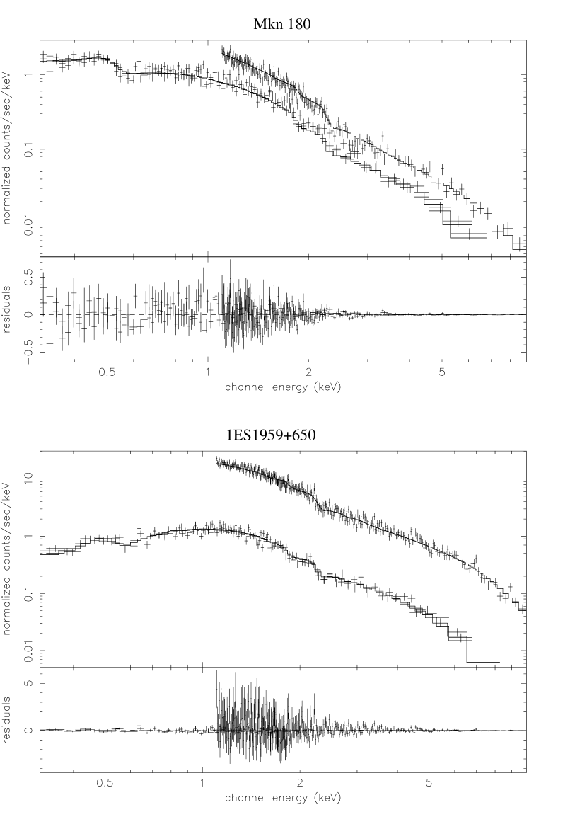
Figure 1.— Two examples of the XMM EPIC spectra. At top, Mkn 180 (OBSID 0094170101) and at bottom, 1ES1959+650 (OBSID 0094383301). In both panels, the EPN data are the top line and the data from the MOS detectors are below. The model shown represents the power law plus variable $N_{H}$ fit. See Sections 2 and 3 for discussion.

Figure 2.— Radio light curves for 1ES 1553+113 (top) and 1ES 1028+511 (bottom), obtained at the University of Michigan Radio Astronomy Observatory. Data at 14.5, 8.0 and 4.8 GHz are denoted by crosses, circles and triangles respectively. Daily averages of the data are shown, with the bars denoting $1\sigma$ error estimates. As seen, both sources vary considerably during the radio observations. See Section 2.1-2.2 for discussion.

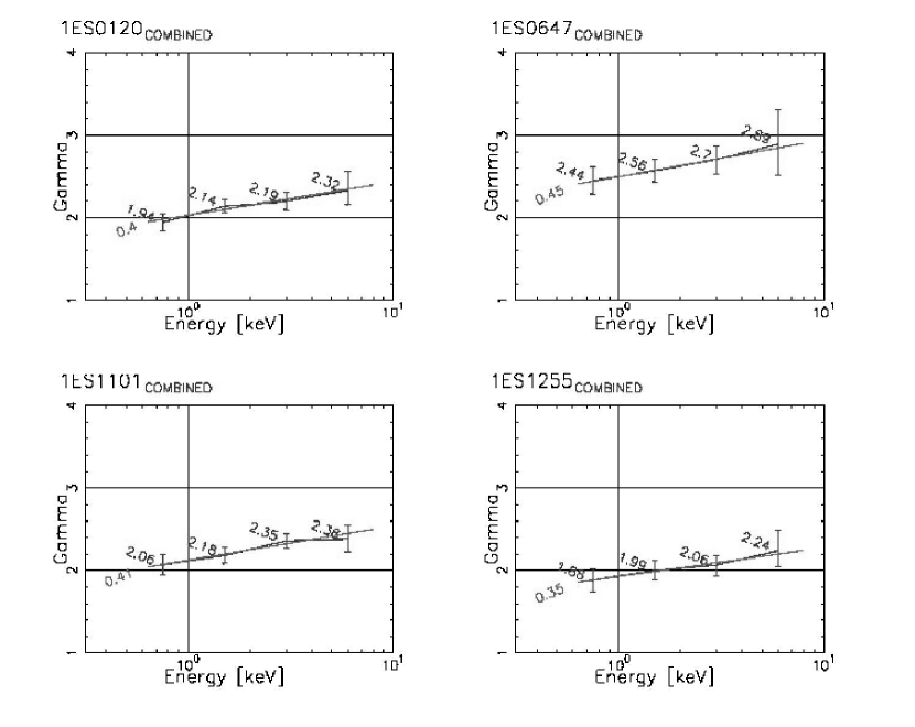
Figure 3.— Four examples of fitting the spectra of BL Lacs in our sample to smaller spectral ranges. All four of these objects show steeper spectra at higher energies, with $d\Gamma/d(logE)\approx 0.4$. See Section 3.3 for discussion.

Figure 4.— Comparison of model fits for the XMM spectrum of 1ES1959+650 (OBSID 0094383301). In the panel at left, the data were fitted with a power-law plus Galactic N(H) model, while at right, the data were fitted with the log-parabola plus Galactic N(H) model. Note that the fit in the left panel is adequate between 1.5–5 keV, but cannot account for the curvature seen both at energies $<1.5$ keV and $>5$ keV. At top, the comparison is shown in terms of the detected spectrum, with each plot showing received spectra plus folded model for the MOS 1 & 2 (bottom lines) and PN (top lines), as well as residual. At bottom, we show the unfolded energy spectrum. These plots show that curvature is present in this spectrum up to the highest energies seen by XMM.

Figure 5.— Plots of the X-ray spectral slope $\Gamma$, versus broadband spectral index $\alpha_{ro}$ (top left) and $\alpha_{ro}$ (top right), as well as the SED peak frequency $\nu_{peak}$ (bottom left). For easy cross-referencing with the Tables, we note in these plots the identity of each point. See Section 4.1 for discussion.

Figure 6.— Plots of $d\Gamma/d(logE)$ versus $\Gamma$ (top) and $\nu_{peak}$ (bottom). For easy cross-referencing with the Tables, we note in these plots the identity of each point. See Section 4.1 for discussion.

Figure 7.— Upper panel: The photon spectrum (solid line) resulting from an episodic injection of electrons in the particle acceleration process. Here $s=3.0$, $E_{max}=100$ KeV, and $E_{1}=50$ KeV. Note that $E_{1}$ is the maximum emitted energy the source is reaching in this episodic mode of injection, while $E_{max}$ is the emitted energy the source would reach under steady injection conditions. For comparison, a power law emission corresponding to an electron distribution with $s=3.0$ is also shown (broken line). Lower panel: the photon index $\Gamma$ that corresponds to the emitted photon spectrum. Note the gradual steepening of the spectrum, manifested by an increase of $\Gamma$ with energy. The dotted lines represent the energy range $0.5-10$ keV covered by XMM. See Section 4.2 for discussion.

Table 1Log of XMM Observations

1ES Name	OBSID	Date	MOS gt	Filter	Frame	Ct Rate	PN gt	Filter	Frame	Ct Rate
			(sec)			(sec)	(sec)			(Ct/s)
0033+595	00943813011	2003-02-01	1500	Thin/Med	PartialW2	1.17	4100	Thin1	Small	3.43
0120+340	0094382101	2002-01-05	5600	Medium	PartialW2	2.43	3500	Medium	Small	8.48
0145+138	0094383401	2002-07-18	4200	Thin1	PartialW2	0.07	3200	Thin1	Small	0.25
0323+022	0094382501	2002-02-05	5200	Medium	PartialW2	0.81	3200	Medium	Small	2.81
0347$-$121	0094381101	2002-08-28	3000	Thin1	PartialW2	3.32	2200	Thin1	Small	11.6
0414+009	0094383101	2002-08-26	5700	Thin1	Partial/ Full	3.18	5600	Thin1	Small	12.1
0647+250	00943809011,2	2002-03-25	2300	Medium	PartialW2	2.10	1900	Medium	Small	7.49
…	0094382901	2002-03-25	N/A	N/A	N/A	N/A	N/A	Medium	Small	N/A
1028+511	00943818011	2001-05-15	N/A	N/A	N/A	N/A	1176	Medium	Small	5.59
…	0094382701	2001-11-26	5600	Medium	PartialW2	4.30	3500	Medium	Small	16.2
1101$-$232	00943806011	2001-05-29	2200	Medium	PartialW2	4.70	4300	Medium	Small	17.6
1133+704	00941703011	2001-04-12	N/A	Thin1	Full	N/A	N/A	Thin1	Full	N/A
…	00941701012	2001-04-12	3300	Thin1	Full	4.45 (2.02) 3	6900	Thin1	Full	12.5 (5.81)3
1255+244	00943830011	2002-12-12	5800	Medium	PartialW2	1.30	4000	Medium	Small	4.40
…	0094383201	2002-06-26	662	Medium	PartialW2	1.35	435	Medium	Small	4.88
1553+113	0094380801	2001-09-06	5000	Medium	PartialW2	13.0 (4.31) 3	3500	Medium	Small	50.5
1959+650	00943802011	2002-11-23	300	Medium	PartialW2	21.2 (5.29)3	N/A	Medium	Small	N/A
…	00943833011	2003-01-16	2200	Medium	PartialW2	10.5 (2.08)3	1200	Medium	Small	39.5
…	0094373501	2003-02-09	3700	Medium	PartialW2	12.5 (3.80) 3	2000	Medium	Small	43.3

Table 2Supporting observations

1ES Name	OBSID	OM Band	F(UV)	$F_{max}$(rad)
			($10^{-16}{\rm~{}erg~{}cm^{-2}~{}s^{-1}~{}\AA^{-1}}$)	(Jy)
0033+595	0094381301	UVW2$\times$2	$<3.3^{1}$	0.3
0120+340	0094382101	UVW2$\times$5	$8.9\pm 0.9$	0.1
0145+138	0094383401	UVW2$\times$4	$<3.3^{1}$	0.2
0323+022	0094382501	UVW2$\times$5	$14.4\pm 1.0$	0.3
0347$-$121	0094381101	UVW2$\times$4	$7.6\pm 2.0$	—2
0414+009	0094383101	UVW2$\times$5	$18.5\pm 0.1$	0.1
0647+250	0094380901	UVW2$\times$1	$<3.3^{1}$	0.1
…	0094382901	UVW2$\times$5	$<3.3^{1}$	0.1
1028+511	0094381801	UVW2$\times$5	$18.2\pm 1.6$	0.2
…	0094382701	UVW2$\times$4	$21.9\pm 0.7$	0.2
1101$-$232	0094380601	UVW2$\times$4	$10\pm 3$	0.3
1133+704	0094170301	N/A	N/A	—2
…	0094170101	U$\times$4	$272\pm 8$	N/A3
1255+244	0094383001	UVW2$\times$5	$3.2\pm 1.5$	0.2
…	0094383201	UVW2$\times$4	$<3.3^{1}$	0.2
1553+113	0094380801	UVW2$\times$5	$185\pm 5$	0.8
1959+650	0094380201	UVW2$\times$5	$35.0\pm 2.0$	0.6
…	0094383301	UVW2$\times$5	$25.3\pm 2.0$	0.6
…	0094373501	UVW2$\times$5	$28.4\pm 2.0$	0.6

Table 3BL Lac Spectral Fit Parameters

1ES Name	ObsId	Fit parameters, N(H) Fixed				Fit parameters, N(H) Free
		$\mathrm{N_{H,Gal}}$	$\Gamma$	$\mathrm{F_{2-10keV}}$	$\chi^{2}$/dof. (dof.)	$\mathrm{N_{H,tot}}$	$\Gamma$	$\mathrm{F_{2-10keV}}$	$\chi^{2}$/dof. (dof.)	$F$-test
		$10^{20}~{}\mathrm{cm^{-2}}$		erg cm-2 s-1		$10^{20}~{}\mathrm{cm^{-2}}$		erg cm-2 s-1		Probability
0033+595	0094381301	42.4	$2.2^{+0.02}_{-0.03}$	$1.2\times 10^{-11}$	1.42(288)	63.8${}^{+3.8}_{-3.6}$	2.47$\pm{0.05}$	1.1$\times 10^{-11}$	1.01(287)	$<10^{-10}$
0120+340	0094382101	5.14	$2.16^{+0.01}_{-0.01}$	$9.7\times 10^{-12}$	1.70(527)	9.9$\pm{0.6}$	2.34${}^{+0.02}_{-0.03}$	8.9$\times 10^{-12}$	1.32(526)	$<10^{-10}$
0145+138	0094383401	5.10	$2.07\pm 0.12$	$2.5\times 10^{-13}$	1.44(88)	22.1${}^{+8.0}_{-6.9}$	2.83${}^{+0.38}_{-0.34}$	1.6$\times 10^{-13}$	1.24(87)	$3.2\times 10^{-4}$
0323+022	0094382501	8.74	$2.54^{+0.02}_{-0.03}$	$2.0\times 10^{-12}$	1.05(213)	11.9$\pm{1.2}$	2.67$\pm{0.06}$	1.9$\times 10^{-12}$	0.95(212)	$1.3\times 10^{-5}$
0347$-$121	0094381101	3.64	$1.77^{+0.02}_{-0.01}$	$1.8\times 10^{-11}$	1.18(530)	5.0$\pm{0.6}$	1.82$\pm{0.03}$	1.8$\times 10^{-11}$	1.16(529)	$2.6\times 10^{-3}$
0414+009	0094383101	10.3	$2.47^{+0.02}_{-0.01}$	$9.3\times 10^{-12}$	1.20(499)	13.1$\pm{0.6}$	2.57$\pm{0.03}$	8.9$\times 10^{-12}$	1.09(498)	$<10^{-10}$
0647+250	0094380901	12.8	$2.62\pm 0.02$	$5.6\times 10^{-12}$	1.36(278)	19.0${}^{+1.2}_{-1.1}$	2.86$\pm{0.05}$	5.0$\times 10^{-12}$	1.05(277)	$<10^{-10}$
1028+511	0094381801	1.16	$2.44^{+0.04}_{-0.03}$	$1.2\times 10^{-11}$	1.20(107)	3.77$\pm{1.1}$	2.61$\pm{0.08}$	1.0$\times 10^{-11}$	1.04(106)	$<10^{-10}$
…	0094382701	1.16	$2.28\pm 0.01$	$1.2\times 10^{-11}$	1.41(600)	5.2$\pm{0.4}$	2.46$\pm{0.02}$	9.7$\times 10^{-12}$	0.98(599)	$<10^{-10}$
1101$-$232	0094380601	5.76	$2.23^{+0.02}_{-0.01}$	$2.3\times 10^{-11}$	1.37(682)	10.9$\pm{0.6}$	2.40${}^{+0.02}_{-0.03}$	2.2$\times 10^{-11}$	1.05(681)	$<10^{-10}$
1133+704	0094170101	1.42	$2.40\pm 0.02$	$9.8\times 10^{-12}$	1.21(361)	1.8$\pm{0.7}$	2.42$\pm{0.04}$	9.7$\times 10^{-12}$	1.20(360)	8.4 $\times 10^{-2}$
1255+244	0094383001	1.26	$1.99^{+0.01}_{-0.02}$	$5.1\times 10^{-12}$	1.18(380)	2.9${}^{+2.9}_{-2.6}$	1.83$\pm{0.12}$	4.8$\times 10^{-12}$	1.02(379)	$<10^{-10}$
…	0094383201	1.26	$1.76^{+0.07}_{-0.06}$	$7.5\times 10^{-12}$	0.97(134)	4.6$\pm{0.8}$	2.11${}^{+0.04}_{-0.03}$	4.8$\times 10^{-12}$	0.97(133)	N/A
1553+513	0094380801	3.67	$2.38\pm 0.01$	$3.5\times 10^{-11}$	1.26(815)	5.7$\pm{0.4}$	2.46${}^{+0.01}_{-0.02}$	3.4$\times 10^{-11}$	1.17(814)	$<10^{-10}$
1959+650	0094380201	10.1	$1.70\pm 0.05$	$2.9\times 10^{-10}$	1.44(58)	13.3${}^{+3.1}_{-2.9}$	1.80${}^{0.1}_{-0.11}$	2.8$\times 10^{-10}$	1.41(57)	0.275
…	0094383301	10.1	$2.10^{+0.02}_{-0.01}$	$7.7\times 10^{-11}$	1.51(514)	17.9$\pm{1.0}$	2.29${}^{+0.02}_{-0.03}$	7.2$\times 10^{-11}$	1.08(513)	$<10^{-10}$
…	0094383501	10.1	$2.02\pm 0.02$	$6.9\times 10^{-11}$	1.64(863)	16.9$\pm{0.6}$	2.18${}^{+0.02}_{-0.01}$	6.5$\times 10^{-11}$	1.13(862)	$<10^{-10}$

Note. — MOS data used in 0.5 - 10.0 keV range PN in 1.1 - 10.0 keV range.

Table 4Parameters for BL Lac Spectral Curvature

		4-band $\Gamma$-Fittinga						Logarithmic Parabolaa
1ES Name	ObsId	$\Gamma_{0.5-1.0keV}$	$\Gamma_{1.0-2.0keV}$	$\Gamma_{2.0-4.0keV}$	$\Gamma_{4.0-10.0keV}$	$\chi 2$/dof. (dof.)   b	$\mathrm{d}\Gamma/\mathrm{d}(logE)$	$\Gamma$	$\beta$	$\chi 2$/dof. (dof.)
0033+595	0094381301	$1.49^{+1.07}_{-1.98}$	$2.03^{+0.18}_{-0.18}$	$2.34^{+0.12}_{-0.12}$	$2.33^{+0.22}_{-0.22}$	$1.04(187)$	$0.58$	$1.71^{0.1}_{-0.09}$	$-0.67^{+0.12}_{-0.13}$	1.10 (287)
0120+340	0094382101	$1.94^{+0.1}_{-0.1}$	$2.14^{+0.08}_{-0.08}$	$2.19^{+0.1}_{-0.09}$	$2.32^{+0.22}_{-0.16}$	$1.16(383)$	$0.4$	$2.05\pm 0.02$	$-0.30\pm 0.04$	1.37 (526)
0145+138	0094383401	$0.25^{+0.86}_{-3.25}$	$2.83^{+0.72}_{-0.66}$	$2.54^{+0.91}_{-0.71}$	$0.16^{+1.12}_{-2.76}$	$1.34(77)$	$-0.76$	$1.84^{+0.17}_{-0.2}$	$-1.26^{+0.56}_{-0.68}$	1.27(87)
0323+022	0094382501	$2.29^{+0.17}_{-0.17}$	$2.6^{+0.15}_{-0.15}$	$2.52^{+0.18}_{-0.19}$	$2.89^{+0.53}_{-0.38}$	$1.03(156)$	$0.47$	$2.48^{+0.03}_{-0.04}$	$-0.22^{+0.09}_{-0.08}$	0.96(212)
0347$-$121	0094381101	$1.6^{+0.12}_{-0.13}$	$1.82^{+0.09}_{-0.09}$	$1.9^{+0.1}_{-0.11}$	$1.75^{+0.13}_{-0.17}$	$1.15(398)$	$0.22$	$1.75^{+0.03}_{-0.02}$	$-0.05^{+0.05}_{-0.04}$	1.18(529)
0414+009	0094383101	$2.4^{+0.11}_{-0.11}$	$2.45^{+0.09}_{-0.09}$	$2.51^{+0.09}_{-0.09}$	$2.82^{+0.18}_{-0.18}$	$1.15(309)$	$0.34$	$2.41\pm 0.02$	$-0.16\pm 0.04$	1.11(498)
0647+250	0094380901	$2.44^{+0.16}_{-0.16}$	$2.56^{+0.13}_{-0.13}$	$2.7^{+0.17}_{-0.18}$	$2.89^{+0.4}_{-0.38}$	$0.89(197)$	$0.45$	$2.5^{+0.03}_{-0.04}$	$-0.39\pm 0.08$	1.10(277)
1028+511	0094382701	$2.23^{+0.07}_{-0.07}$	$2.23^{+0.07}_{-0.06}$	$2.49^{+0.09}_{-0.09}$	$2.48^{+0.17}_{-0.17}$	$0.93(425)$	$0.36$	$2.20\pm 0.01$	$-0.30\pm 0.03$	1.00(599)
…	0094381801c	—	—	—	—	—	—	— $2.42\pm 0.04$	$-0.19^{+0.10}_{-0.12}$	1.13(106)
1101$-$232	0094380601	$2.06^{+0.12}_{-0.12}$	$2.18^{+0.09}_{-0.09}$	$2.35^{+0.08}_{-0.08}$	$2.38^{+0.16}_{-0.15}$	$0.93(472)$	$0.41$	$2.09\pm 0.02$	$-0.32^{+0.03}_{-0.04}$	1.05(681)
1133+704	0094170101	$2.3^{+0.14}_{-0.14}$	$2.21^{+0.14}_{-0.14}$	$2.34^{+0.14}_{-0.14}$	$2.47^{+0.28}_{-0.27}$	$1.28(223)$	$0.14$	$2.39^{+0.03}_{-0.02}$	$-0.01^{+0.05}_{-0.06}$	1.21 (360)
1255+244	0094383001	$1.88\pm{0.13}$	$1.99\pm 0.11$	$2.06^{+0.12}_{-0.13}$	$2.24^{+0.25}_{-0.18}$	$0.97(283)$	$-0.5$	$1.90^{+0.03}_{-0.02}$	$-0.22\pm 0.05$	1.05(379)
…	0094383201	$2.29^{+0.48}_{-0.49}$	$1.70\pm 0.37$	$1.71^{+0.41}_{-0.45}$	$1.08^{+0.58}_{-0.71}$	$0.84(112)$	$0.35$	$1.76^{+0.10}_{-0.10}$	$-0.01^{+0.18}_{-0.21}$	0.98(133)
1553+113	0094380801	$2.35^{+0.07}_{-0.07}$	$2.25^{+0.07}_{-0.07}$	$2.42^{+0.06}_{-0.06}$	$2.44^{+0.12}_{-0.12}$	$1.11(603)$	$0.14$	$2.33^{+0.02}_{-0.01}$	$-0.13^{+0.02}_{-0.03}$	1.17(814)
1959+650	0094380201	$1.34^{+0.33}_{-0.35}$	$1.78^{+0.25}_{-0.25}$	$1.87^{+0.32}_{-0.31}$	$1.29^{+0.6}_{-0.6}$	$1.45(57)$	$0.31$	$1.64\pm{0.10}$	$-0.14^{+0.18}_{-0.19}$	1.43(57)
…	0094383301	$1.75^{+0.19}_{-0.19}$	$2.14^{+0.12}_{-0.12}$	$2.21^{+0.09}_{-0.09}$	$2.36^{+0.16}_{-0.16}$	$1.11(331)$	$0.57$	$1.88^{+0.04}_{-0.03}$	$-0.39\pm 0.05$	1.14(513)
…	0094383501	$1.86^{+0.11}_{-0.11}$	$1.89^{+0.07}_{-0.07}$	$2.11^{+0.06}_{-0.06}$	$2.36^{+0.1}_{-0.1}$	$1.05(653)$	$0.59$	$1.81\pm{0.02}$	$-0.37^{+0.03}_{-0.04}$	1.13(862)

Table 5Discrete features found in RGS Spectra

1ES Namea	OBSID	Energy (keV)	$\Delta\chi^{2}$	Width (eV)	Comments
1ES0033+595	0094381301	1.07	$-12.02$	$45^{+20}_{-24}$	MOS 2 + 1 RGS only
1ES1101$-$232	0094380601	0.67	$-18.56$	$7^{+4}_{-3}$	RGS 2 only
1ES1101$-$232	0094380601	1.36	$-16.62$	$22\pm 9$	RGS 2 only
1ES1255$+$244	0094383201	1.29	$-11.98$	$30\pm 16$	MOS 1, MOS 2 but not in RGS
1ES1255$+$244	0094383201	2.91	$-8.91$	$8^{+6}_{-4}$	Single MOS 1&2 channel, instrumental?
1ES1959$+$650	0094383301	1.92	$-11.77$	$<18$	Two RGS 1 channels, not RGS 2 or MOS

Table 6Multiwaveband Parameters

1ES Name	OBSID	$\alpha_{RO}$	$\alpha_{OX}$	log $\nu_{peak}$	Comments
0033+595	0094381301	0.70	0.66	17.17	Converges poorly; radio flux had to be lowered artificially
0120+340	0094382101	0.56	0.97	17.17
0145+138	0094383401	0.59	1.44	14.48
0323+022	0094382501	0.49	1.29	15.12	Confusing radio source? Catalog flux 25% of UMRAO value
0347$-$121	0094381101	0.29	0.93	17.99	$\alpha_{x}<1$ – use log $\nu_{peak}$=18.
0414+009	0094383101	0.39	0.99	16.33
0647+250	0094380901	0.36	1.18	16.28	Catalog optical flux 15x brighter than OM data
0647+250	0094382901	0.36	1.18	16.28	Catalog optical flux 15x brighter than OM data
1028+511	0094381801	0.42	0.96	16.51
…	0094382701	0.47	1.07	16.21
1101$-$232	0094380601	0.45	0.67	17.57
1133+704	0094170301	0.26	1.38	15.13
1255+244	0094383001	0.53	0.82	16.60	Catalog opt flux 25x brighter than OM; increased opt flux $2\times$
…	0094383201	0.53	0.82	18.00	$\alpha_{x}<1$ – use log $\nu_{peak}=18$.
1553+113	0094380801	0.32	1.16	15.70
1959+650	0094380201	0.47	0.63	18.00	$\alpha_{x}<1$ – use log $\nu_{peak}=18$.
…	0094383301	0.48	0.72	18.00	Used log $\nu_{peak}=18$ even though object not in flare.
…	0094373501	0.48	0.79	18.00	Used log $\nu_{peak}=18$ even though object not in flare.

References

- (1) Aller, H. D., Aller, M. F., Latimer, G. E., Hodge, P. E. , 1985, ApJS, 59, 513
- (2) Andersson, K. E., Madejski, G. M., 2004, ApJ, 607, 190
- (3) Beckmann, V., Wolter, A., Celotti, A., Costamante, L., Ghisellini, G., Maccacaro, T., Tagliaferri, G., 2002, A&A 383, 410
- (4) Blustin, A. J., Page, M. J. Branduardi-Raymont, G., 2004, A& A 417, 61
- (5) Boller, T., Gliozzi, M., Griffiths, G., Sembay, S., Keil, R., Schwentker, O., Brinkmann, W., & Vercellone, S., 2001, A&A, 365, L158
- (6) Cagnoni, I., Nicastro, F., Maraschi, L., Treves, A., Tavecchio, F., 2004, ApJ, 603, 449
- (7) Canizares, C. R., Kruper, J., 1984, ApJL, 278, 99
- (8) Elvis, M., Plummer, D., Schachter, J., & Fabbiano, G., 1992, ApJS, 80, 257
- (9) Gallant, Y. A. 2002, in Relativistic Flows in Astrophysics, ed. A. W. Guthmann, M. Georganopoulos, A. Marcowith, & K. Manolakou (Lecture Notes in Phys. 589; Berlin: Springer), 24
- (10) Giommi, P., Capalbi, M., Fiocchi, M., Memola, E., Perri, M., Piranomonte, S., Rebecchi, S., Massaro, E., 2002, in Blazar Astrophysics with BeppoSAX and Other Observatories, ed. P. Giommi, E. Massaro & G. Palumbo (Roma: ESA/ASI), 63
- (11) Goudfrooij, P., de Jong, T., Hansen, L., Norgaard-Nielson, H. U., 1994, MNRAS, 271, 833
- (12) Guainazzi, M., Vacanti, G., Malizia, A., O’Flaherty, K. S., Palazzi, E., Parmar, A. N., 1999, A&A, 342, 124
- (13) Harris, D. E., Biretta, J. A., Junor, W., Perlman, E. S., Sparks, W. B., & Wilson, A. S., 2003, ApJ, 586, L41
- (14) Inoue, S. & Takahara, F., 1996, ApJ, 463, 555
- (15) Iwasawa, K., Fabian, A., and Nandra, K. 1999, MNRAS, 307, 611
- (16) Jannuzi, B. T., Smith, P. S., Elston, R., 1994, ApJ, 428, 130
- (17) Jansen, F., et al. 2001, A&A 365, L1
- (18) Kinney, A. L., Bohlin, R. C., Blades, J. C., & York, D. G., 1991, ApJS, 75, 645
- (19) Kirk, J. G., Rieger, F. M., Mastichiadis, A. 1997, A&A, 333, 452
- (20) Krawczynski, H., et al. 2004, ApJ, 601, 151
- (21) Kubo, H., Takahashi, T., Madejski, G., Tashiro, M., Makino, F., Inoue, S., Takahara, F., 1998, ApJ, 504, 693
- (22) Lamer, G., Brunner, H., Staubert, R., 1996, A&A 327, 467
- (23) Landau, R., et al., 1986, ApJL, 307, L78
- (24) Lanzetta, K., Turnshek, D. A., & Sandoval, J., 1993, ApJS, 84, 109
- (25) Leahy, J. P., 1991, in Beams and Jets in Astrophysics, ed. P. A. Hughes (Cambridge: Cambridge University Press), p. 100
- (26) Madejski, G. M., Mushotzky, R. F., Weaver, K. A., Arnaud, K. A., Urry, C. M., 1991, ApJ, 370, 198
- (27) Madejski, G. M., et al., 1992, in Proc. Yamada Conference XXVIII, ed. Y. Tanaka & K. Koyama, Frontiers Science Series (Tokyo: Universal Academy Press), 583
- (28) Massaro, E., 2002, in Blazar Astrophysics with BeppoSAX and Other Observatories, ed. P. Giommi, E. Massaro & G. Palumbo (Roma: ESA/ASI), 3
- (29) Massaro, E., Perri, M., Giommi, P., Nesci, R., Verrechia, F., 2004a, A& A, 422, 103
- (30) Massaro, E., Perri, M., Giommi, P., Nesci, R., 2004b, A& A, 413, 489
- (31) McKernan, B., Yaqoob, T., Reynolds, C. S., 2004, ApJ, in press, astro-ph/0408506
- (32) Morrison, R., McCammonn, D., 1983, ApJ, 270, 119
- (33) Nicastro et al., 2002, ApJ, 573, 157
- (34) Pacholczyk, A. G., 1970, Radio Astrophysics (San Fransisco: Freeman)
- (35) Padovani, P., Costamante, L., Giommi, P., Ghisellini, G., Celotti, A., Wolter, A., 2004, MNRAS, 347, 1282
- (36) Padovani, P., et al., 2001, MNRAS, 328, 931
- (37) Padovani, P., Giommi, P., Fiore, F., 1997, MNRAS, 284, 569
- (38) Penton, S., Shull, J. M., 1996, unpublished IUE AGN database, online at http://origins.colorado.edu/iueagn
- (39) Perlman, E. S., et al., 1996b, ApJS, 104, 251
- (40) Perlman, E. S., Harris, D. E., Biretta, J. A., Sparks, W. B., Macchetto, F. D., 2003, ApJ, 599, L65
- (41) Perlman, E. S., Madejski, G., Stocke, J. T., Rector, T. A., 1999, ApJ, 523, L11
- (42) Perlman, E. S., Stocke, J. T., Wang, Q. D., Morris, S. L., 1996a, ApJ, 465, 1010
- (43) Perlman, E. S., Wilson, A. S., 2005, ApJ, in press.
- (44) Read, A. M., Ponman, T. J., 2003, A& A, 409, 395
- (45) Rector, T. A. Stocke, J. T., 2001, AJ, 122, 565
- (46) Rector, T. A., Stocke, J. T., Perlman, E. S., Morris, S. L., Gioia, I. M., 2000, AJ, 120, 1626
- (47) Rybicki, G. B., Lightman, A. P., 1979, Radiative Processes in Astrophysics (Wiley-Interscience: New York).
- (48) Sambruna, R. M., Barr, P., Giommi, P., Maraschi, L., Tagliaferri, G., Treves, A., 1994, ApJS, 95, 371
- (49) Sambruna, R. M., Maraschi, L., Urry, C. M., 1996, ApJ, 463, 444
- (50) Sambruna, R. M., George, I. M., Madejski, G., Urry, C. M., Turner, T. J., Weaver, K. A., Maraschi, L., Treves, A., 1997, ApJ, 483, 774
- (51) Sambruna, R. M., & Mushotzky , R. F., 1998, ApJ, 502, 630
- (52) Stark, A. A., Gammie, C. F., Wilson, R. W., Bally, J., Linke, R. A., Heiles, C., Hurwitz, M., 1992, ApJS, 79, 77
- (53) Takahashi, T., et al. 1996, ApJ, 470, L89
- (54) Tanihata, C., et al., 2001, ApJ, 563, 569
- (55) Tavecchio, F., Maraschi, L., Ghisellini, G., 1998, ApJ, 509, 608
- (56) Ulrich, M.–H., Maraschi, L., Urry, C. M., 1997, ARAA, 45, 445
- (57) Urry, C. M., Mushotzky, R. F., and Holt, S. S. 1986, ApJ, 305, 369
- (58) Urry, C. M., Padovani, P., 1995, PASP, 107, 803
- (59) Urry, C. M., Sambruma, R. M., Worrall, D. M., Kollgaard, R. I., Feigelson, E. D., Perlman, E. S., Stocke, J. T., 1996, ApJ, 463, 424
- (60) Wolter, A., et al., 1998, A&A, 335, 899
- (61) Worrall, D. M., WIlkes, B. J., 1990, ApJ, 360, 396
- (62)