A semi-relativistic approach to the circular restricted three body problem and a numerical experiment around the 3:2 resonance

Abstract

A Hamiltonian that approaches the study of the three-body problem in general relativity is obtained. We use it to study the relativistic version of the circular restricted three-body problem in which the first body is the heaviest and the third body is a test-particle. We focus on the orbits around the 3:2 resonance. We show that, in spite of the notable difference between the relativistic and Newtonian orbits, most of the resonant region is preserved. Nevertheless, differently from the Newtonian case, the frequencies between the second and the third body are no longer commensurable.

1 Introduction

In the Newtonian context, the restricted three body problem has been widely studied in order to predict resonances in the solar system dynamics, specially concerning the motion of comets and asteroids (see for instance [1, 2, 3]). By definition, the third body is a test particle that does not gravitationally affect the motion of the other two bodies that are in a Keplerian motion. A typical example is the study of the motion of the asteroids between Jupiter and the Sun, considered to be the first two bodies. Most of these asteroids are in a mean-motion resonance with Jupiter [4]. An interesting problem is the existence of gaps in the distribution of semi-major axes of the orbits of asteroids - the Kirkwood gap. Wisdom solved this problem by studying the orbits near the 3:1 commensurability [5]. Regarding the three body problem we may also cite the problem of the Hannay angle [6, 7] and a new exact solution obtained by Chenciner and Montgomery [8].

Perhaps the first article concerning the n-body problem in General Relativity was written by De Sitter [9] in the very beginning of the last century and his predictions about the precession of the Moon was confirmed by Shapiro et al [10]. In a relativistic framework, approximations are always needed in order to study the gravitational field generated by more than one body. Post-Newtonian approaches were employed several times in the three body problem, one may cite the work from Krefetz [11] in which a solution corresponding to the equilateral Lagrange one is obtained. Also, Rosswog and Trautmann [12] studied the Lagrangian stability points for the circular problem. Brumberg [13] has considered such problem in a radiating binary system. Using a different approach, Guéron and Letelier [14] considered the interaction among orbiting particles around a black hole. We also may cite the work from Campanelli et al [15] where the influence of a very massive black hole in the stability of binary systems by means of Post-Newtonian techniques was studied.

In this article, I introduce a novel formalism to account for the General Relativistic effects on the n-body problem for systems so that there is a predominant very massive body, for instance, a super massive black hole as the one in the center of the Milky Way [16]. The technique presented is based on the Hamiltonian formalism for the geodesic problem. The gravitational effects of the heaviest source are associated to an exact solution of the Einstein field equations and the field of the other bodies perturbs the corresponding Hamiltonian as a classical gravitational potential energy but does not affect the motion of the heaviest body. Therefore equations of motion obtained describe the trajectory of the light bodies. We can compare the method proposed here with the ones used to compute relativistic secular effects in the orbits of solar system objects [17]. In this procedure the mean relativistic corrections are given continuously with the Hamiltonian, differently to other approaches in which such effects are considered periodically in the correction of the planetary orbits.

As a first test to this formalism, the restricted and circular three body problem is numerically studied. For this purpose, the Schwarzschild solution is associated to the heaviest source (hereafter the first body). The computed Hamiltonian is changed by the potential energy generated by a second body in a circular geodesic motion around the first and the equations of motion of a test-particle (third body) affected by these two bodies are derived. The stability of the orbits around the 3:2 central resonance is studied by means of Poincaré sections. This specific choice is justifiable since chaotic regions are clearly distinguished from resonant islands in the circular problem. It was found that the general relativistic effects destroy the commensurability of the frequencies of the orbits of the second and the third bodies mainly for eccentric orbits. Remarkably, most of the resonant regions are preserved. In other words, it means that most of the orbits that were stable in the Newtonian limit remains stable when relativistic effects are considered. Nonetheless the ratio between the motion period of the second body and the period of the motion of the third one is no longer a rational number.

2 Hamiltonian Formalism

Given a metric tensor $g_{\mu\nu}$, the geodesic equations in General Relativity are equivalent to the Euler-Lagrange ones obtained from the Lagrangian

$${\mathcal{L}}=\sqrt{|g_{\mu\nu}u^{\mu}u^{\nu}|},$$ (1)

$u^{\mu}=dx^{\mu}/d\tau$ and the units are so that $c=1$ and $G=1$. The Einstein sum convention is adopted and Greek and Latin indices vary respectively from 0 to 3 and 1 to 3.

Usually the equations of motion are written with an affine parameter, i.e., a free variable proportional to the arc length (for instance the proper time $\tau$). Sometimes, however, the use of a non-affine parameter becomes necessary. For this purpose, one must derive the corresponding formulation to the geodesic problem. A typical example of a non-affine useful parameter is the coordinate time. When the evolution of more than one particle is to be compared, $t$ as a free parameter seems to be more adequate.

In order to write the Hamiltonian for a test particle whose orbit is parameterized by a time-like coordinate, one starts with the action

$$S=\int p_{\mu}dx^{\mu}=\int\left(p_{0}+p_{i}\frac{dx^{i}}{dt}\right)dt,$$ (2)

where $p_{\mu}=mg_{\mu\nu}\frac{dx^{\nu}}{d\tau}$. Recalling the Legendre transformation $H=p_{i}\frac{dx^{i}}{dt}-{\mathcal{L}}$ one may identify $H=-p_{0}$.

Writing $p_{0}$ as a function of the other components (the relation $g^{\mu\nu}p_{\nu}p_{\mu}=-m^{2}$ was considered) one gets the Hamiltonian:

$$H(p_{i},x^{j},t)=\frac{g^{0i}}{g_{00}}+\left(\frac{(g^{ij}p_{i}p_{j}+m^{2})}{-g^{00}}+\left(\frac{g^{0i}p_{i}}{g^{00}}\right)^{2}\right)^{1/2}.$$ (3)

This formulae is general and we only require $t$ to be a time-like coordinate. For more details about this formulae see the Refs. [18, 19].

Now let us suppose that besides the gravitational field generated by the central source, there are smaller sources that affect the motion of the test particle. The matter we have now is how to include such field in the Hamiltonian formalism. Assuming that these sources are much lighter than the main source, one can compute their contribution by adding a perturbative term in the above given Hamiltonian Eq. (3). The natural choice is the Newtonian gravitational potential.

Then I propose that for a system with a heavy source (or a predominant mean field) and $n$ smaller massive bodies, can be approximated by the following Hamiltonian:

$$H(p_{i},x^{j},t)=\frac{g^{0i}}{g_{00}}+\left(\frac{(g^{ij}p_{i}p_{j}+1)}{-g^{00}}+\left(\frac{g^{0i}p_{i}}{g^{00}}\right)^{2}\right)^{1/2}-\sum^{n}_{k=1}\frac{\mu_{k}}{|\mathbf{r}_{k}-\mathbf{r}|},$$ (4)

where $\mu_{k}$ is the mass of the $k^{th}$ body. Notice that the dependence on the mass of the test particle was eliminated.

2.1 Limits of applicability

The approximation presented above is quite simple. The Newtonian potential is added to the exact relativistic Hamiltonian that leads to the geodesic equations parameterized by the coordinate time. Therefore it is not difficult to enumerate the relativistic effects that are not being considered in this approach. First one must have in mind that in the exact solution there should be a lot of “mixed” terms in the Hamiltonian due to the nonlinearity of the Einstein equations - in the Newtonian approach they do not exist. A didactic example is the solution of two static black holes sustained by a string or a strut [20, 21]. The metric and hence the Hamiltonian are much more complicated than a simple sum of potential energies. Also, terms due to the non-staticity of the solution are not being considered, the obvious neglected effect is the damping by gravitational radiation [22, 23, 24, 26].

Although these terms are very important in some astrophysical systems (see for instance [25, 27, 28]), the largest error corresponds to the fact that all the source but the central one are considered Newtonian. We may say that the method can be used when $\sum_{i}^{N}(M/d_{0i})\gg\sum_{i<j}^{N}(m_{i}/d_{ij})$ that is the relativistic effects due to the central source are much more important than the relativistic contributions from the lighter bodies ($d_{0i}$ is the $i^{th}$ particle distance to the central body and $d_{ij}$ between the $i^{th}$ and the $j^{th}$ orbiting particles supposing $m_{i}\geq m_{j}$). Notice that, since the first term of the function (4) is associated to a mean gravitational field, an average of some relativistic effects due to the orbiting bodies might be computed in the Hamiltonian. An example is the use of multipolar solution [29, 30].

A simple idea for estimating the error starts with the Schwarzschild metric $ds^{2}=(1-2M/r)dt^{2}-1/(1-2M/r)dr^{2}+r^{2}d\Omega^{2}$ (that will be better explored in the next sections). We could think that in the full general relativistic solution, the perturbative term would be similar to the first one. This, of course, is not true due to the nonlinearity of the Einstein equations. Nevertheless, it may be used to estimate the order of magnitude of the error we are doing. For the Schwarzschild metric above written we have that

$$[g^{\mu\nu}]={\rm diag}\left[1/(1-2M/r),1-2M/r,(r\sin\theta)^{-2},r^{-2}\right]$$ (5)

Now, if the motion of the particle is restricted to the plane $\theta=\pi/2$ we will have that $p_{\theta}=0$. With these assumptions, we might expand the expression corresponding to Hamiltonian of a single particle with planar motion in the Schwarzschild line element substituting (5) in (3):

$$H_{s}=\sqrt{(1-2m/r)((1-2m/r)p_{r}^{2}+p_{\varphi}^{2}/r^{2}+1)}.$$ (6)

The first relativistic term is of the order $m^{2}/r^{2}$ in geometric units. Roughly speaking this term has the order of magnitude of the error done in the simulations.

2.2 Schwarzschild

The particular system I am interested in this paper concerns planar motions around a black hole (all the considered bodies are in the same plane). The Hamiltonian for a free particle around a Schwarzschild black hole with mass $M$ can be cast as:

$$H=\sqrt{(1-2M/r)((1-2M/r)p_{r}^{2}+p_{\varphi}^{2}/r^{2}+1)},$$ (7)

in which usual spherical coordinates are used.

The Hamilton equations obtained from the above function will give the geodesic motion of a test particle orbiting around a static and non charged black hole. Since I want to study the motion of a third body that is attracted by the central source and the orbiting body. It will be considered that the force exerted by the second body on the third one is essentially Newtonian. For this achieving, one assumes that the central source is fixed and the motion of the second body is given by the time-like geodesic around the first one represented by the curve ${\bf r_{2}}(t)$. Using these assumptions, we may write a Hamiltonian that approximates the motion of the third body by adding the contribution of the second body as a Newtonian gravitational potential energy to Eq.7. Thus the proposed Hamiltonian has the form

$$H=\sqrt{(1-2M/r)((1-2M/r)p_{r}^{2}+p_{\varphi}^{2}/r^{2}+1)}-\frac{m}{|{\bf r}-{\bf r_{2}}(t)|}.$$ (8)

(M and m are the masses of the first and second bodies respectively)

Summarizing, the first term of this Hamiltonian represents the geodesic motion of a test-particle around a spherical symmetric source and the second is the gravitational potential generated by an orbiting body. Therefore, the Hamilton-Jacobi equations lead to the equations of motion of the test-particle (Remind that in this particular example all the three bodies are in the same plane)

3 Simulations

I intend to make an analysis of the orbits by means of the study of surfaces of sections in the phase space. Since the Hamiltonian is time-dependent, it is useful to study periodic orbits of the second body in order to eliminate this dependence. Nevertheless, periodic orbits are not easily found in time-like geodesics around a black hole except when the test particle experiments a circular motion. Therefore it is interesting to study the restricted three body problem when the second orbit is circular, i.e., when the second body has the motion

$$\varphi_{2}=\omega t,\>\>\>r_{2}=\mbox{constant.}$$ (9)

Substituting Eq.9 in Eq.8 one gets the Hamiltonian that describes the motion of the third body in this particular case

$$\!\!\!\!\!\!\!\!\!\!\!\!\!\!\!\!\!\!\!\!\!\!\!\!\!\!H=\sqrt{(1-2m/r)((1-2m/r)p_{r}^{2}+p_{\varphi}^{2}/r^{2}+1)}-\frac{m}{\sqrt{r^{2}+r_{2}^{2}-2rr_{2}\cos(\omega t-\varphi)}}.$$ (10)

It is clear that $H$ is not a constant of motion because of its time dependence . However by means of the simple conjugate transformation of coordinates [5] $\varphi^{\prime}=\omega t-\varphi$ (the other coordinates do not transform) one writes a new Hamiltonian $K$ that is constant

$$\!\!\!\!\!\!\!\!\!\!\!\!\!\!\!\!\!\!\!\!\!\!\!\!\!\!\!\!\!\!\!\!K=\sqrt{(1-2M/r)((1-2M/r)p_{r}^{2}+p_{\varphi}^{2}/r^{2}+1)}+\omega p_{\varphi}-\frac{m}{\sqrt{r^{2}+r_{2}^{2}-2rr_{2}\cos(\varphi^{\prime})}}$$ (11)

The constant angular speed of the second body $\omega$ may be calculated from Eq.7 and $g_{\mu\nu}u^{\mu}u^{\nu}=-1$. One gets that $\omega=\frac{d\varphi_{2}}{dt}=\sqrt{\frac{m}{r_{2}^{3}}}$ - exactly the same value obtained in the Newtonian analogue.

With a constant Hamiltonian the problem now has two degrees of freedom. Therefore it is easy to make a study on the stability by means of Poincaré sections. For this purpose I mark the position where an orbit crosses the plane defined by $\varphi-\omega t=\varphi^{\prime}=2k\pi$, i.e., when the test-particle and the second body are in the same angular position ($k$ is an integer).

The first step is the determination of the constant $K$ that defines a three dimensional hypersurface in the phase space inside which the motion must be confined. For this purpose, I calculate the parameters of the circular geodesic whose period is 2/3 of the period the second. This requirement gives us $r$ and $p_{\varphi}$. Those values with the parameters of the second body are used to fix $K$ in the simulations. Note that $K$ can be associated to the Jacobi’s usually computed in restricted three body problem [1, 3].

After fixing $K$ as described above, I determine a set of initial conditions in order to plot the Poincaré section - there are three free variables to be chosen. Each figure to be presented is associated to a fixed $K$ and out of them it was considered $m/M=10^{-3}$. For distances of the order of 10 Schwarzschild radii to the second body (units defined with respect to the first body), the error will be of the order of $10^{-6}$.

The procedure adopted to plot the Poincaré section has an important characteristic: If we had the Newtonian problem, all the Poincaré sections would present exactly the same aspect. In other words they correspond to the same Jacobi constant. When we change proportionally the initial positions and velocities of the bodies without changing their masses, we obtain qualitatively the same situation in the Newton gravitational problem but a different situation in the relativistic problem.

The Poincaré sections are then presented in Fig.1-2. In all the figures, the abscissa is the radial coordinate (the distance of the test particle to the central mass) and the ordinate is its conjugated momentum. Both are computed when $\varphi-\omega t=\varphi^{\prime}=2k\pi$ as described above.

In Fig.1, the relativistic aspects do not play an important role since the orbiting bodies are very distant from the central source thus one has a typical surface of section for the classical problem - notice that indirectly the Newtonian limit of the Eq.10 is tested here. Some resonant regions are presented and the eccentricity of the test-particle orbits increases as I increase the rate $\langle d\varphi/dt\rangle/\omega$. The circular orbit are inside the $3/2$ resonant island. I mark the 3:2 resonant island A, 5:3 with B and 2:1 with C.(Along this paper only mean orbital resonances are considered.) These values are determined by computing $\langle d\varphi/dt\rangle/\omega$, it means that the period of motion of the second body is 3/2 times the period of the test particle (third body) when they do not interact. Since the points of the surface section are marked when the orbits are in conjunction with respect to the central source, if they are in a $R:S$ resonance, the number of stable islands will be $|R-S|$.

Repeating the procedure we get the Fig.2 in which the orbits are very close to the central source and the relativistic effects are important. Nevertheless, most of the stable islands are preserved. It is clear that the islands corresponding to the 3:2, 5:3 and 2:1 resonances are preserved when compared to the Fig.1. (In this case the ratios between the periods in the resonant islands are not necessarily commensurable as we will discuss later.)

Another important aspect concerns chaotic orbits. Close to the central source they tend to fill a larger portion of the phase space comparing with the Newtonian case. In a extreme case, i.e., very close to the central source or for huge masses of the first body, the only bounded orbits are the ones that belong to some resonant region, thus, almost all the chaotic orbits become unbounded, see Fig.3.

Some orbits of the test-particle are presented. For the constants presented in Fig.3, the unbounded orbits tend to fall into the black hole as we see in Fig.5. Similar initial conditions but using constants defined in Fig.2 lead to bounded orbits as presented in Fig.4.

A remarkable result concerns the commensurability of the stable orbits. For a typical Newtonian situation (similar to the one presented in Fig.1) the stable islands usually correspond to regions of commensurability of periods, i.e., the ratio between the frequency of any orbit inside this region and the frequency of the second body (that is fixed) is a rational number. However, when the general relativistic effects increase this assumption is generally not true although the stable islands are not easily destroyed as we see in Fig.2. Therefore the ratio between the period of the test-particle and second body orbits gradually departs from the rational number obtained in the Newtonian limit. We shall notice that even close to the black hole, there is one specific real number corresponding to each stable island. (The numerical error when two different orbits in the same island are compared is smaller than typical fluctuations of the integration routine.) We present a curve of the ratio between the orbital frequency of the test-particle and the second body inside the region corresponding to the Newtonian 2:1 resonance, Fig.6. The ordinate is the angular speed of the test-particle divided by the orbital frequency of the second body (this value is computed after many cycles). The abscissa is the distance between the second body and the central source (because it moves circularly). It is very clear that the ratio tends to 2 when $r\rightarrow\infty$ (the Newtonian limit) and decreases as much as we approach the source. This behavior is similar in all the stable islands preserved close to the black hole except inside the 3:2 region where, by construction, the commensurability remains.

4 Final Remarks

Although other resonances were studied, the particular case of the circular restricted three body problem presented in this article happens to be the most interesting because large chaotic regions are observed in the Newtonian case. When we study orbits around the central 2:1 resonance, for instance, a small chaotic region is noticed for eccentric orbits computed very close to the central source. Anyway, nothing more remarkable is obtained in the circular restricted three body problem close to other resonances.

Despite only few examples of the restricted three body problem were studied, I conjecture that the result concerning the resonant islands is general. Imagine a situation in which massive objects are growing by collisions similarly to the planetary formation process [32]. In this sort of process, lots of particles of dust remain after some time. From the results here presented it is possible to argue that most of the particles were captured by the black hole (similar to what is shown in the Fig.3) because of the perturbative influence of other bodies. On the other hand the objects formed during this process should stay in a resonant region (otherwise they would not be formed). Certainly, a more specific and complete work must be done in order to verify this speculation. Since the technique is based on a Hamiltonian formalism, symplectic maps should be used in order to study such complex systems.

I shall emphasize that the proposed technique may be employed (carefully) in different contexts. The mainly condition is the predominance of the mean gravitational field associated to the metric. An interesting application of this method consists in the evolution of self-interacting systems in a cosmological background (see for instance the study of formation of binaries performed by Ioka et al [33]). At last I may say that the aim of this article was mainly to present a new approach to study relativistic effects in some astrophysical systems and the new results concerning the three body problem although interesting were important to test the method rather than presenting a great novelty in general relativity.

References

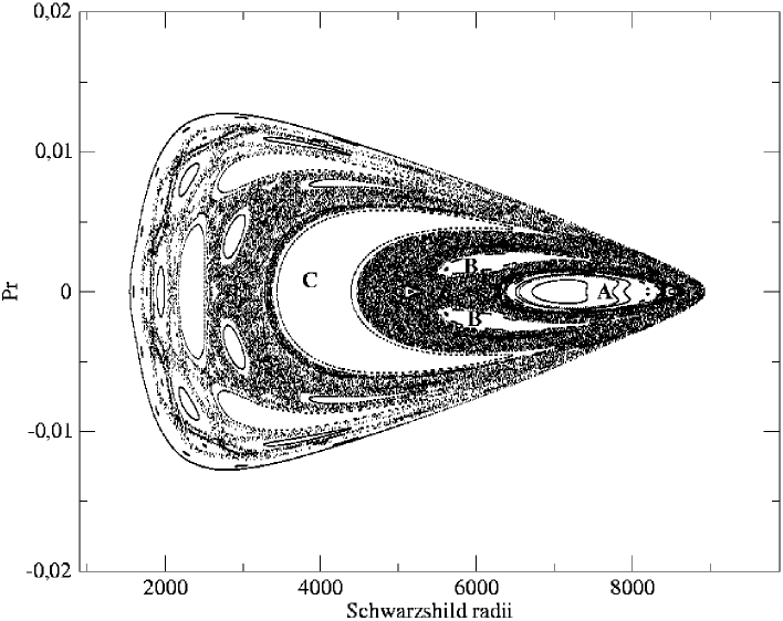
Figure 1: Surface of section distant to the black hole, $K=0.9998$. The radius of the circular orbit $r_{2}=10^{4}$ (see Eq.11 ). The ordinate is the radial component of the momentum and in the abscissas one has the distance of the test-particle to the central mass. In this example a situation where the relativistic effects do not play an important role. The resonant regions are very clear. For example, I mark A - 3:2, B - 5:3 and C - 2:1 resonances

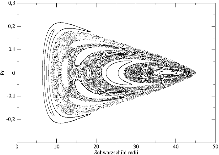
Figure 2: For $K=0.969$, the particles are much closer to the central source and relativistic effects are very important, $r_{2}=50$. In spite of that, most of the stable islands are preserved when compared to the previous figure.

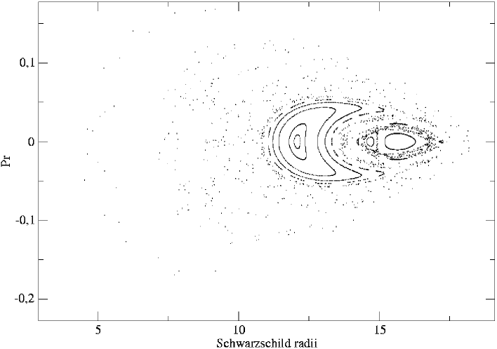
Figure 3: In this very relativistic situation ($K=0.92076$, $r_{2}=20$) we see that the only bounded orbits are the ones that belong to a resonant region.

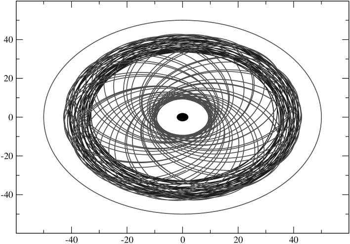
Figure 4: A chaotic orbit and a regular one between the trajectory of the second body and the black hole are plotted (the orbits are in the $x-y$ plane). It is clear that both are bounded.

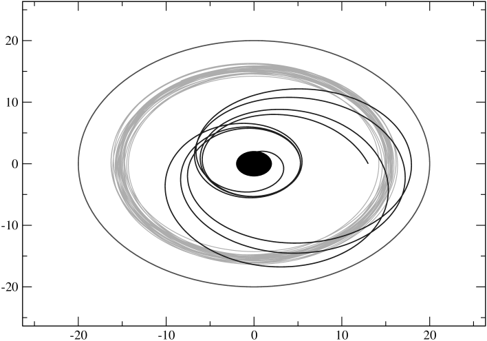
Figure 5: Now the orbits are a little bit closer to the black hole. Looking to the orbital plane we see that the regular orbits remain bounded while the chaotic ones falls into the black hole. This situation corresponds to the one presented in the Fig.3

.

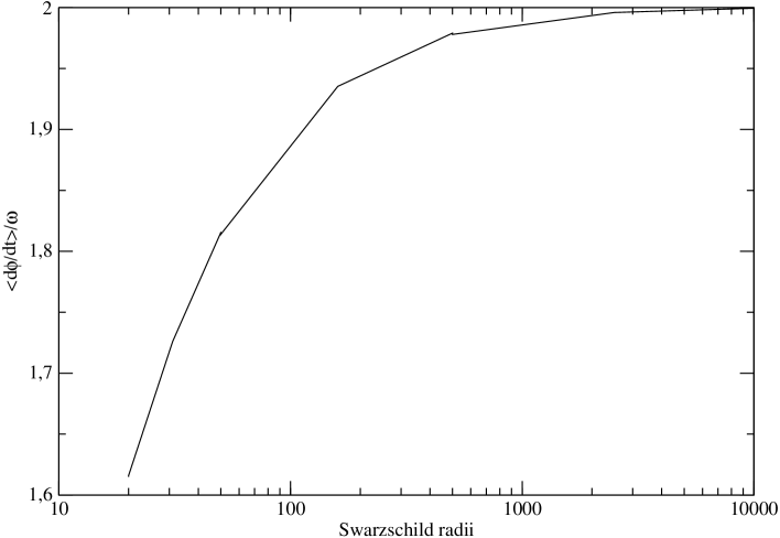
Figure 6: Here we have $\langle d\varphi/dt\rangle/\omega$ obtained for orbits that are, in the Newtonian limit, inside the 2:1 resonant region. For large distances to the central mass the ratio of the mean orbital frequency is almost 2 whereas near the source (larger relativistic contributions) this ratio decreases (indicating loss of commensurability).

References

- [1] Danby, J.M.A. “Fundamentals Of Celestial Mechanics (Willmann-Bell, 1988)
-
[2]
Murray, C.D. and Dermott, S.F. “Solar System Dynamics”
(Cambridge Univ. Press 1999)
Morbidelli, A. “Modern Celestial Mechanics: Dynamics in the Solar System” (Taylor & Francis, 2002) - [3] Henon, M. 1966, IAUS 25 157
- [4] Lemaitre, A. and Henrard, J. 1989, Cel. Mech 43 91
- [5] Wisdom, J. AJ, 87 577
- [6] Hannay, J. 1985 J. Phys. A: Math. Gen. 18, 221.
- [7] Spallicci A., Morbidelli A., Metris G., 2005 Nonlinearity 18 45.
- [8] Chenciner A, Montgomery R. 2000 Ann. Math 152 881.
-
[9]
De Sitter, W. 1916 MNRAS, 77, 155;
De Sitter, W. 1917 MNRAS 77 481 . - [10] Shapiro I.I., Reasenberg R.D., Chandler J.F. and Babcock R.W. 1988 Phys. Rev. Lett.61 2643
- [11] Krefetz, E. 1967 AJ, 72 471
- [12] Rosswog, S. and Trautmann, D. 1996 Planet. Space Sci. 44 313
- [13] Brumberg, V.A. Cel. Mech, 85 269
- [14] Guéron, E. and Letelier, P.S. 2004 Gen. Rel. Grav. 36 2107-2122
- [15] Campanelli, M. Dettwyler, M. Mark Hannam,M and Lousto C.O. astro-ph/0509814
- [16] Ghez, A.M. Morris, M Becklin, M. E. E. Tanner, A. and Kremenek, T. 2000, Nature 407 (21), 349
-
[17]
Wisdom J and Holman M. 1991. Astron. J. 102 1528
Laskar, J. and Robutel, P. 2001 Cel. Mec. Dyn. Astron.80 39 - [18] Wald, Robert M. General Relativity. (Chicago, 1984)
- [19] Bertschinger, E. “Hamiltonian Dynamics of Particle Motion” Lecture Notes - 8.962 (Massachusetts Institute of Technology, 2002)
- [20] Kramer, D. and Neugebauer, G. 1980, Phys. Lett. A
- [21] Gueron, E. and Letelier, P.S. “Weyl Solutions: Solitons, Strings and Struts” in Procedings of Silarg VIII (World Scientific, Singapore, 1994) 75 : 259-261
- [22] Cooperstock, F. I. and Booth, D. J. 1969, Phys. Rev. 187 1796
- [23] Hulse, R.A. and Taylor, J. H. 1975, Astrophys. J. 195 L51
- [24] Barack, L. and Burko, L. M. 2000 Phys Rev. D 62 084040
- [25] Barack, L. and Lousto, C. O. 2002 Phys Rev. D 66 061502
- [26] Quinn, T.C. and Wald R. M. 1997 Phys Rev. D 56 3381
- [27] Mino, Y., Sasaki M. and Tanaka T. 1997 Phys Rev. D 55 3457
- [28] Spallicci A. and Aoudia S. 2004 Class. Quantum Grav.21 S563
- [29] Quevedo, H. 1989 Phys. Rev. D, 39 2904-2911
- [30] Boisseau, B. and Letelier, P.S. 2002, Gen. Rel. Grav. 34 1077-1096
- [31] Abramowicz, M.A. Bulik, T. Bursa, M. and Kluźniak, W. 2003 Astron. Astroph. 404, L21 L24
- [32] Lecar, M. and S.J. Aarseth, S.J. 1986 Astroph. J. 305 564
- [33] Kunihito Ioka, K Chiba, T. Tanaka, T. and Nakamura, T. 1998, Phys. Rev. D 58 063003.
- [34] Burnell, F. Malecki, J. J. Mann, R. B. and Oht, T. Phys. Rev. E 69, 016214 (2004)
.