Magnetic field generation from cosmological perturbations

Abstract

In this letter, we discuss generation of magnetic field from cosmological perturbations. We consider the evolution of three component plasma (electron, proton and photon) evaluating the collision term between elecrons and photons up to the second order. The collision term is shown to induce electric current, which then generate magnetic field. There are three contributions, two of which can be evaluated from the first-order quantities, while the other one is fluid vorticity which is purely second order. We estimate the magnitudes of the former contributions and shows that the amplitude of the produced magnetic field is about $\sim 10^{-19}{\rm G}$ at 10Mpc comoving scale at the decoupling. Compared to astrophysical and inflationary mechanisms for seed-field generation, our study suffers from much less ambiguities concerning unknown physics and/or processes.

I Introduction

There are convincing evidences that imply existence of substantial magnetic fields in various astronomical objects. Not only galaxies but systems with even larger scales, such as cluster of galaxies and extra-cluster fields, have their own magnetic fields (for a review on cosmological magnetic fields, see e.g., Widrow02 ). Conventionally the magnetic fields in galaxies, and possibly in clusters of galaxies, are considered to have been amplified and maintained by dynamo mechanism. However, the dynamo mechanism needs the seed magnetic field and does not explain the origin of the magnetic fields.

There have been many attempts to generate the seed fields. One of the approaches to this problem is to generate magnetic fields astrophysically, often involving the Biermann mechanism Biermann50 . This mechanism has been applied to various systems: large-scale structure formation Kulsrud97 , ionizing front Gnedin00 , protogalaxies Davies00 and supernova remnant of the first stars Hanayama05 . These studies showed the possibilities of magnetic-field generation with amplitudes of order $10^{-16}\sim 10^{-21}{\rm G}$, which would be enough for the required field $\sim 10^{-20}{\rm G}$.

On the other hand, cosmological origins, which are often concerned with inflation, can produce magnetic field with coherence lengths of much larger scales, which is typically the horizon scale or possibly super-horizon scale Turner88 ; Bamba04 ; Ashoorioon04 ; Bertolami99 ; Bertolami05 . Also they can often produce fields with a wide range of length scales, while astrophysical mechanisms can produce fields only with their characteristic scales. For a constraints on magnetic field with cosmological scale, see Yamazaki04 .

In this Letter, we consider magnetic-field generation from cosmological perturbations after inflation. Around and after the decoupling, coupling among charged particles and photons become so weak that electric current can be induced by the difference in motions of protons and electrons. This electric current leads to generation of magnetic fields. It is well known that vorticity of plasma produces such electric current Harrison70 ; Lesch95 ; Hogan00 ; Berezhiani04 ; Matarrese04 ; Gopal04 . However, because vorticity is not produced at the first order in cosmological perturbations, we must study the second order. We will consider equations of motion for protons, electrons and photons separately up to the second order, although equation of motion for photons does not appear explicitly. To study electric current appropriately, we must treat the three components separately Gopal04 . Furthermore, we will evaluate the collision term between electrons and photons, which is dominant and essential for the magnetic-field generation, up to the second order. From the equations of motion for protons and electrons, we obtain a generalized Ohm’s law, which, combined with the Maxwell equations, leads to an evolution equation for magnetic field. Our study is based on the cosmological perturbation theory, which is highly successful in the anisotropies of the cosmic microwave background, and suffers from much less ambiguities concerning unknown physics and/or processes compared to astrophysical and inflationary mechanisms for seed-field generation. Thus our results are robust.

II Formulation

Euler equations for proton fluid and electron fluid are given by

$$(\delta^{i}_{~{}\mu}+u^{i}u_{\mu})\left(T^{\mu\nu}_{p~{};\nu}+T^{\mu\nu}_{{\rm EM}p;\nu}\right)=C^{(C)i}_{pe}+C^{(T)i}_{p\gamma},$$ (1)

$$(\delta^{i}_{~{}\mu}+u^{i}u_{\mu})\left(T^{\mu\nu}_{e~{};\nu}+T^{\mu\nu}_{{\rm EM}e;\nu}\right)=C^{(C)i}_{ep}+C^{(T)i}_{e\gamma},$$ (2)

where $T^{\mu\nu}_{p(e)}$ and $T^{\mu\nu}_{{\rm EM}p(e)}$ are the energy-momentum tensor of proton (electron) fluid and electromagnetic field coupling to protons (electrons) current, respectively. Here $\mu,\nu=0,1,2,3$ and $i=1,2,3$. The projection of the divergence of the energy-momentum tensors are computed as

$$(\delta^{i}_{~{}\mu}+u^{i}u_{\mu})T^{\mu\nu}_{~{}~{};\nu}$$

$$~{}~{}~{}~{}=(\rho+p)u^{\mu}u^{i}_{~{};\mu}+(\delta^{i}_{~{}\mu}+u^{i}u_{\mu})P^{,\mu},$$ (3)

$$(\delta^{i}_{~{}\mu}+u^{i}u_{\mu})T^{\mu\nu}_{{\rm EM};\nu}=-j^{\nu}F^{\mu}_{~{}~{}\nu},$$ (4)

where $\rho$, $P$ and $j^{\mu}$ are the energy density, pressure and electric current, respectively. The r.h.s. of Eq. (1) and (2) represent the collision terms. $C^{(C)\mu}_{pe}=-C^{(C)\mu}_{ep}$ is the collision term for the Coulomb scattering between protons and electrons. This term leads to the diffusion of magnetic field and can be neglected in the highly conducting medium in early universe. On the other hand, the collsion terms for the Thomson scattering between protons (electrons) and photons are expressed as $C^{(T)\mu}_{p(e)\gamma}$. Because the collision term for the protons can be neglected compared to that for the electrons, difference in velocities of protons and electrons will be induced which leads to electric current. This electric current becomes a source for magnetic field.

Now we evaluate the collision term for the Thomson scattering:

$$\gamma(p_{i})+e^{-}(q_{i})\rightarrow\gamma(p^{\prime}_{i})+e^{-}(q^{\prime}_{i}),$$ (5)

where the quantities in the parentheses denote the particle momenta. The collision integral $C^{(T)}_{\gamma e}[f(p_{i})]$ for this scattering is given as

$$C^{(T)}_{\gamma e}[f(p_{i})] = \frac{2\pi^{4}}{p}\int\frac{d^{3}p^{\prime}}{(2\pi)^{3}2E_{\gamma}(p^{\prime})}\int\frac{d^{3}q}{(2\pi)^{3}2E_{e}(q)}\int\frac{d^{3}q^{\prime}}{(2\pi)^{3}2E_{e}(q^{\prime})}$$ (6)

$$\times|M|^{2}\delta\left[E_{\gamma}(p)+E_{e}(q)-E_{\gamma}(p^{\prime})-E_{e}(q^{\prime})\right]\delta^{(3)}\left[p_{i}+q_{i}-p^{\prime}_{i}-q^{\prime}_{i}\right]\left\{f_{\gamma}(p^{\prime}_{i})f_{e}(q^{\prime}_{i})-f_{\gamma}(p_{i})f_{e}(q_{i})\right\}$$

$$\sim \frac{\pi n_{e}}{4m_{e}^{2}p}\int\frac{d^{3}p^{\prime}}{(2\pi)^{3}p^{\prime}}|M|^{2}\left\{f_{\gamma}(p^{\prime}_{i})-f_{\gamma}(p_{i})\right\}\left\{\delta(p-p^{\prime})+(p_{i}-p^{\prime}_{i})u_{e}^{i}\frac{\partial\delta(p-p^{\prime})}{\partial p^{\prime}}\right\},$$

where $E_{\gamma(e)}$ and $f_{\gamma(e)}$ are the energy and the distribution function of photons (electrons), respectively, $|M|^{2}$ is the scattering amplitude and $m_{e}$ is the electron mass. Then we obtain the collision term in the Euler equation (2), as

$$C^{(T)i}_{\gamma e}[f(p_{i})] = \int\frac{d^{3}p}{(2\pi)^{3}}p^{i}C^{(T)}_{\gamma e}[f(p_{i})]$$ (7)

$$= \frac{4\sigma_{T}\rho_{\gamma}n_{e}}{3}\left[(u_{e}^{i}-u_{\gamma}^{i})+\frac{1}{8}u_{ej}\Pi_{\gamma}^{ij}\right],$$

where $\sigma_{T}$ is the cross section of the Thomson scattering. Here moments of the distribution functions are given by

$$\int\frac{d^{3}p}{(2\pi)^{3}}pf_{\gamma}(p_{i})=\rho_{\gamma},$$ (8)

$$\int\frac{d^{3}p}{(2\pi)^{3}}p^{i}f_{\gamma}(p_{i})=\frac{4}{3}\rho_{\gamma}u_{\gamma}^{i},$$ (9)

$$\int\frac{d^{3}p}{(2\pi)^{3}}p^{i}f_{e}(p_{i})=\rho_{e}u_{e}^{i},$$ (10)

$$\int\frac{d^{3}p}{(2\pi)^{3}}p^{-1}p^{i}p^{j}f_{\gamma}(p_{i})=\frac{1}{6}\rho_{\gamma}\Pi_{\gamma}^{ij}+\frac{1}{3}\rho_{\gamma}\delta^{ij},$$ (11)

where $\Pi_{\gamma}^{ij}$ is photon anisotropic stress. It should be noted that the collision term (7) was obtained non-perturbatively with respect to the cosmological perturbation.

Altogether, the Euler equations for protons and electrons are written as

$$m_{p}nu_{p}^{\mu}u_{p;\mu}^{i}-enu_{p}^{\mu}F_{\mu}^{~{}i}=0,$$ (12)

$$m_{e}nu_{e}^{\mu}u_{e;\mu}^{i}+enu_{e}^{\mu}F_{\mu}^{~{}i}$$

$$~{}~{}=-\frac{4\sigma_{T}\rho_{\gamma}n}{3}\left[(u_{e}^{i}-u_{\gamma}^{i})+\frac{1}{8}u_{ej}\Pi_{\gamma}^{ij}\right],$$ (13)

where $m_{p}$ is the proton mass, and the pressure of proton and electron fluids are neglected. We also assumed the charge neutrality: $n=n_{e}\sim n_{p}$. Subtracting Eq. (12) multiplied by $m_{e}$ from Eq. (13) multiplied by $m_{p}$, we obtain

$$-\frac{m_{p}m_{e}}{e}\left[nu^{\mu}\left(\frac{j^{i}}{n}\right)_{;\mu}+j^{\mu}\left(\frac{m_{p}-m_{e}}{m_{p}+m_{e}}\frac{j^{i}}{en}-u^{i}\right)_{;\mu}\right]$$

$$+en(m_{p}+m_{e})u^{\mu}F^{i}_{~{}\mu}-(m_{p}-m_{e})j^{\mu}F^{i}_{~{}\mu}$$

$$=-\frac{4m_{p}\sigma_{T}\rho_{\gamma}n}{3}\left[(u_{e}^{i}-u_{\gamma}^{i})+\frac{1}{8}u_{ej}\Pi_{\gamma}^{ij}\right],$$ (14)

where $u^{\mu}$ and $j^{\mu}$ are the center-of-mass 4-velocity of the proton and electron fluids and the net electric current, respectively, defined as

$$u^{\mu}\equiv\frac{m_{p}u_{p}^{\mu}+m_{e}u_{e}^{\mu}}{m_{p}+m_{e}},$$ (15)

$$j^{\mu}\equiv en(u_{p}^{\mu}-u_{e}^{\mu}).$$ (16)

Noting the Maxwell equations $F^{\mu\nu}_{;\nu}=j^{\mu}$, we see that the first term in the l.h.s. of Eq. (14) are suppressed, compared to the second term, by a factor Subramanian94

$$\frac{c^{2}}{L^{2}\omega_{p}^{2}}\sim 3\times 10^{-47}\left(\frac{10^{10}{\rm cm}^{-3}}{n}\right)\left(\frac{1{\rm Mpc}}{L}\right)^{2},$$ (17)

where $c$ is the speed of light, $L$ is a characteristic length of the system and $\omega_{p}=\sqrt{4\pi ne^{2}/m_{e}}$ is the plasma frequency. Second order vector perturbations are contained in the covariant derivative of the electric current and were evaluated in Matarrese04 . They obtained the current magnetic field of order $10^{-29}{\rm G}$ at 1Mpc scale. As we will see below, this is much smaller than a value we obtain in this paper, which justifies the neglection of the first term in the l.h.s. of Eq. (14).

The third term in the l.h.s. of Eq. (14) is the Hall term which can also be neglected because the Coulomb coupling between protons and electrons is so tight that $|u^{i}|\gg|u_{p}^{i}-u_{e}^{i}|$. Then we have a generalized Ohm’s law:

$$u^{\mu}F^{i}_{~{}\mu}=-\frac{4\sigma_{T}\rho_{\gamma}}{3e}\left[(u_{e}^{i}-u_{\gamma}^{i})+\frac{1}{8}u_{ej}\Pi_{\gamma}^{ij}\right]\equiv C^{i}.$$ (18)

Now we derive the evolution equation for magnetic field. This can be obtained from the Bianchi identities $F_{[\mu\nu,\lambda]}=0$, as

$$0 = \epsilon^{ijk}u^{\mu}F_{[jk,\mu]}$$ (19)

$$= u^{\mu}B^{i}_{~{}\mu}-\frac{1}{u^{0}}\epsilon^{ijk}C_{j}u^{0}_{~{},k}+\epsilon^{ijk}C_{j,k}$$

$$-(u^{i}_{~{},j}B^{j}-u^{j}_{~{},j}B^{i})+\frac{u^{0}_{~{},j}}{u^{0}}(B^{j}u^{i}-B^{i}u^{j}),$$

where $\epsilon^{ijk}$ is the Levi-Cività tensor and $B^{i}\equiv\epsilon^{ijk}F_{jk}/2$ is comoving magnetic field. We can expand the photon energy density, fluid velosities and photon anisotropic stress as

$$\rho_{\gamma}=\stackrel{{\scriptstyle\mbox{\tiny(0)}}}{{\rho}}_{\gamma}+\stackrel{{\scriptstyle\mbox{\tiny(1)}}}{{\rho}}_{\gamma}+\cdots,~{}~{}~{}u_{0}=1+\stackrel{{\scriptstyle\mbox{\tiny(2)}}}{{u}}_{0}+\cdots,$$

$$u_{i}=\stackrel{{\scriptstyle\mbox{\tiny(1)}}}{{u}}_{i}+\stackrel{{\scriptstyle\mbox{\tiny(2)}}}{{u}}_{i}+\cdots,~{}~{}~{}\Pi_{\gamma}^{ij}=\stackrel{{\scriptstyle\mbox{\tiny(1)}}}{{\Pi}}_{\gamma}^{ij}+\cdots,$$ (20)

where the superscripts $(i)$ denote the order of expansion. Remembering that $B^{i}$ is a small quantity, we see that most of the terms in Eq. (19), other than the first and third terms, can be neglected. Thus we obtain

$$\dot{B}^{i} \sim -\epsilon^{ijk}C_{j,k}$$ (21)

$$\sim \frac{4\sigma_{T}\stackrel{{\scriptstyle\mbox{\tiny(0)}}}{{\rho}}_{\gamma}}{3e}\epsilon^{ijk}\Biggl{[}\frac{\stackrel{{\scriptstyle\mbox{\tiny(1)}}}{{\rho}}_{\gamma,k}}{\stackrel{{\scriptstyle\mbox{\tiny(0)}}}{{\rho}}_{\gamma}}\left(\stackrel{{\scriptstyle\mbox{\tiny(1)}}}{{u}}_{ej}-\stackrel{{\scriptstyle\mbox{\tiny(1)}}}{{u}}_{\gamma j}\right)+\left(\stackrel{{\scriptstyle\mbox{\tiny(2)}}}{{u}}_{ej,k}-\stackrel{{\scriptstyle\mbox{\tiny(2)}}}{{u}}_{\gamma j,k}\right)$$

$$+\frac{1}{8}\left(\stackrel{{\scriptstyle\mbox{\tiny(1)}}}{{u}}_{el,k}\stackrel{{\scriptstyle\mbox{\tiny(1)}}}{{\Pi}}{}^{l}_{\gamma j}+\stackrel{{\scriptstyle\mbox{\tiny(1)}}}{{u}}_{el}\stackrel{{\scriptstyle\mbox{\tiny(1)}}}{{\Pi}}{}^{l}_{\gamma j,k}\right)\Biggr{]},$$

where the dot denotes a derivative with respect to the cosmic time, and we used the fact that there is no vorticity in the linear order: $\epsilon^{ijk}\stackrel{{\scriptstyle\mbox{\tiny(1)}}}{{u}}_{j,k}=0$. The contributions of the first two terms in Eq. (21) were first noticed in Gopal04 . From this expression, we see that magnetic field cannot be generated in the linear order. Here it should be noted that the velocity of electron fluid can be approximated to the center-of-mass velocity at this order, $\stackrel{{\scriptstyle\mbox{\tiny(1)}}}{{u}}_{e}^{i}\sim\stackrel{{\scriptstyle\mbox{\tiny(1)}}}{{u}}^{i}$.

The linear-order quantities have only scalar components so that we can write as

$$\stackrel{{\scriptstyle\mbox{\tiny(1)}}}{{u}}_{e}^{i}\sim\stackrel{{\scriptstyle\mbox{\tiny(1)}}}{{u}}^{i}=-i\hat{k}^{i}u,~{}~{}~{}~{}\stackrel{{\scriptstyle\mbox{\tiny(1)}}}{{u}}_{\gamma}^{i}=-i\hat{k}^{i}u_{\gamma},$$ (22)

$$\stackrel{{\scriptstyle\mbox{\tiny(1)}}}{{\Pi}}{}^{i}_{\gamma j}=-(\hat{k}^{i}\hat{k}_{j}-\frac{1}{3}\delta^{i}_{~{}j})\Pi_{\gamma},$$ (23)

Also we define $\bar{\rho}_{\gamma}\equiv\stackrel{{\scriptstyle\mbox{\tiny(0)}}}{{\rho}}_{\gamma}$ and $\delta_{\gamma}\equiv\stackrel{{\scriptstyle\mbox{\tiny(1)}}}{{\rho}}_{\gamma}/\bar{\rho}_{\gamma}$. Then we can rewrite the Fourier component of $B^{i}$ in terms of the Fourier components of $\delta_{\gamma}$, $u$, $u_{\gamma}$ and $\Pi_{\gamma}$, as

$$B^{i}(K,t) = \frac{4\sigma_{T}}{3e}\epsilon^{ijk}\int^{t}dt^{\prime}\bar{\rho}_{\gamma}(t^{\prime})\int\frac{d^{3}k^{\prime}}{(2\pi)^{3}}k^{\prime}_{j}K_{k}\bigg{[}\delta_{\gamma}(|\vec{K}-\vec{k}^{\prime}|,t^{\prime})\delta u_{b\gamma}(k^{\prime},t^{\prime})-\frac{3\vec{K}\cdot\vec{k}^{\prime}-2k^{\prime}{}^{2}}{24k^{\prime}{}^{2}|\vec{K}-\vec{k}^{\prime}|}u(|\vec{K}-\vec{k}^{\prime}|,t^{\prime})\Pi_{\gamma}(k^{\prime},t^{\prime})\bigg{]}$$ (24)

$$-\frac{4\sigma_{T}}{3e}\int^{t}dt^{\prime}\bar{\rho}_{\gamma}(t^{\prime})\left[\Omega^{i}(K,t^{\prime})-\Omega_{\gamma}^{i}(K,t^{\prime})\right],$$

where $\hat{k}_{i}$ is the unit vector in direction of $k_{i}$, $\delta u\equiv u-u_{\gamma}$. Vorticities, which come from the second-order vector perturbation, are defined as $\Omega^{i}=\epsilon^{ijk}\stackrel{{\scriptstyle\mbox{\tiny(2)}}}{{u}}_{k,j}$ and $\Omega_{\gamma}^{i}=\epsilon^{ijk}\stackrel{{\scriptstyle\mbox{\tiny(2)}}}{{u}}_{\gamma k,j}$. Eq. (24), which describes the evolution of magnetic field, is one of our main results.

III Evaluation of source terms

Here we briefly evaluate the first two terms in the r.h.s. of Eq. (24) which are constructed from the first-order quantities. The evaluation can be easily accomplished by using linearized Boltzmann code such as CMBFAST cmbfast . In figure 1 we show the power spectra of these terms multiplied by $k$, $kP_{\delta u}(k)$ and $kP_{\Pi u}(k)$, around the last scattering epoch $z\approx 1100$. Here the power spectra are defined as

$$\left<|\delta_{\gamma}(\vec{k})\{u-u_{\gamma}\}(\vec{k}^{\prime})|\right>=P_{\delta u}(k)\delta^{(3)}(\vec{k}-\vec{k}^{\prime})$$ (25)

$$\left<|\Pi_{\gamma}(\vec{k})u(\vec{k}^{\prime})|\right>=P_{\Pi u}(k)\delta^{(3)}(\vec{k}-\vec{k}^{\prime}).$$ (26)

For this illustration all cosmological parameters were fixed to the $\Lambda$CDM values, i.e., $(h,n_{s},\Omega_{b}h^{2},\Omega_{\Lambda},A)=(0.71,0.99,0.022,0.74,0.83)$.

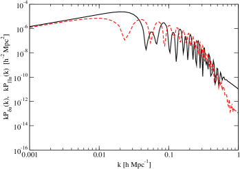
Figure 1: Power spectra (multiplied by $k$) in the source term of Eq.(24) at $z\approx 1100$. The solid and dashed lines correspond to power spectra of $\left<|\delta_{\gamma}(u-u_{\gamma})|\right>$ and $\left<|\Pi_{\gamma}u|\right>$, respectively. The spectra have been normalized to agree on large scales at present epoch.

We found that these two terms contribute to the generation of magnetic field at almost the same order of magnitude at all scales. This can be understood since $\delta_{\gamma}\sim u_{\gamma}$ (acoustic oscillations), $u-u_{\gamma}\sim\varepsilon Ru$, and $\Pi_{\gamma}\sim\varepsilon u_{\gamma}$ in the tight coupling approximation of baryon-photon fluid, where $\varepsilon$ being tight coupling parameter and $R=3\rho_{b}/4\rho_{\gamma}\sim{\cal O}(1)$ around the last scattering epoch. From the spectra we can estimate the field strength of generated magnetic field at the decoupling epoch as $B\sim\frac{8\sigma_{T}a\rho_{\gamma}}{3e}k^{3}P_{\delta u}(k)\sim 10^{-19}{\rm G}$ at 10Mpc comoving scale. If the magnetic field decays adiabatically according to the cosmic expansion, the current magnetic field is about $10^{-25}{\rm G}$.

IV Discussion and summary

In this letter, we discussed generation of magnetic field from cosmological perturbations. Separate treatment of protons, electrons and photons, and appropriate evaluation of collision term allowed us to obtain the evolution equation for magnetic field. We saw that electric current would be induced by collision term between electrons and photons. Up to the second order, there are three contributions which act as sources for magnetic field. In addition to well-known vorticity effect, we found a contribution from the anisotropic stress of photons. Then we estimated the magnitudes of two of the three contributions which can be evaluated from the first-order quantities. We showed the two contributions are comparable at all order and the amplitude of the produced magnetic field is about $10^{-19}{\rm G}$ at 10Mpc comoving scale at the decoupling. Concerning these two contributions, power spectrum of the produced magnetic fields and correlation with the cosmic microwave background must be studied. We will present them elsewhere soon Ichiki05 .

To evaluate the vorticity term, second-order perturbation theory is necessary. Although many authors have been trying this Bruni97 ; Matarrese98 ; Nakamura:2004wr ; Tomita05 , the complete formulation including matter perturbations is still a challenging problem.

K. T. and K. I. are supported by Grant-in-Aid for JSPS Fellows.

References

• (1) L. M. Widrow, Rev. Mod. Phys. 74 (2002) 775.
• (2) L. Biermann, Z. Naturforsch. 5a (1950) 65.
• (3) R. M. Kulsrud, R. Cen, J. P. Ostriker and D. Ryu, Astrophys. J. 480 (1997) 481.
• (4) N. Y. Gnedin, A. Ferrara and E. G. Zweibel, Astrophys. J. 539 (2000) 505.
• (5) G. Davies and L. M. Widrow, Astrophys. J. 540 (2000) 755.
• (6) H. Hanayama, K. Takahashi, K. Kotake, M. Oguri, K. Ichiki and H. Ohno, astro-ph/0501538.
• (7) M. S. Turner and L. M. Widrow, Phys. Rev. D 37 (1988) 2743.
• (8) K. Bamba and J. Yokoyama, Phys. Rev. D 69 (2004) 043507.
• (9) A. Ashoorioon and R. B. Mann, gr-qc/0410053.
• (10) O. Bertolami and D. Mota, Phys. Lett. B 455 (1999) 96.
• (11) O. Bertolami and R. Monteiro, astro-ph/0504211.
• (12) D. G. Yamazaki, K. Ichiki and T. Kajino, astro-ph/0410142.
• (13) E. R. Harrison, Mon. Not. Roy. Astron. Soc. 147 (1970) 279.
• (14) C. Hogan, astro-ph/0005380.
• (15) Z. Berezhiani, A. D. Dolgov, Astropart.Phys. 21 (2004) 59.
• (16) S. Matarrese, S. Mollerach, A. Notari and A. Riotto, Phys. Rev. D 71 (2005) 043502.
• (17) R. Gopal and S. Sethi, astro-ph/0411170.
• (18) H. Lesch and M. Chiba, Astron. Astrophys. 297 (1995) 305.
• (19) K. Subramanian, D. Narasimha and S. M. Chitre, Mon. Not. Roy. Astron. Soc. 271 (1994) L15.
• (20) U. Seljak and M. Zaldarriaga, Astrophys. J., 469, 437 (1996).
• (21) K. Ichiki, K. Takahashi, H. Ohno, H. Hanayama and N. Sugiyama, in preparation.
• (22) M. Bruni, S. Matarrese, S. Mollerach and S. Sonego, Class. Quant. Grav. 14 (1997) 2585.
• (23) S. Matarrese, S. Mollerach and M. Bruni, Phys. Rev. D 58 (1998) 043504-1.
• (24) K. Nakamura, Prog. Theor. Phys. 113 (2005) 481.
• (25) K. Tomita, astro-ph/0501663.