Wide-field weak lensing by RXJ1347–1145
Abstract
We present an analysis of weak lensing observations for RXJ1347–1145 over a field taken in and filters on the Blanco 4m telescope at CTIO. RXJ1347–1145 is a massive cluster at redshift . Using a population of galaxies with , we detect a weak lensing signal at the level, finding best-fit parameters of km s-1 for a singular isothermal sphere model and Mpc with for a NFW model in an , cosmology. In addition, a mass to light ratio M/ was determined. These values are consistent with the previous weak lensing study of RXJ1347–1145 by Fischer & Tyson (1997), giving strong evidence that systemic bias was not introduced by the relatively small field of view in that study. Our best-fit parameter values are also consistent with recent X-ray studies by Allen et al. (2002) and Ettori et al. (2001) but are not consistent with recent optical velocity dispersion measurements by Cohen & Kneib (2002).
1 Introduction
In this paper, we present recent weak lensing observations and analysis of RXJ1347-1145, the most luminous galaxy cluster in the ROSAT All Sky Survey (Schindler et al., 1995), which lies at a redshift of . RXJ1347-1145 has been the subject of numerous observations, including a previous weak lensing study by Fischer & Tyson (1997), and several X-ray and optical studies. The primary purpose of the wide-field weak lensing observation presented in this paper is to test and confirm the earlier gravitational lensing observations of Fischer & Tyson (1997).
Early gravitational lensing studies of RXJ1347-1145 determined a different total mass than early X-ray studies. Such observed disparities for a large and luminous cluster like RXJ1347-1145 raised the possibility of potential systemic problems in methodology. As galaxy cluster mass distributions are a useful probe for dark matter models, the lensing, X-ray, and optical communities independently sought better observations of this cluster.
Fischer & Tyson (1997) studied RXJ1347-1145 through weak lensing analysis of data taken on the Blanco 4m telescope at CTIO using the prime focus CCD camera in 1995. Using an approximately field of view, they found that the mass interior to a 1 Mpc radius was . Assuming an isotropic velocity distribution, this mass corresponded to a velocity dispersion of km s-1.
The results of Fischer & Tyson (1997) were not consistent with the X-ray results of Schindler et al. (1997), who concluded that the temperature of the cluster was keV. As their study presented no evidence that there was a temperature drop from the center of the cluster, Schindler et al. (1997) assumed a constant temperature to find that the total mass within 1 Mpc was .
There were several, independent concerns regarding these weak lensing and X-ray studies that led to further observations. The primary concern for the X-ray studies was the constant temperature assumption in the presence of an apparent large cooling flow. For the weak lensing studies, there was a possibility that the relatively small field of view would introduce a systematic bias, as the outer weak lensing measurements directly influence the predicted interior mass.
Since 1997, several X-ray studies of RXJ1347-1145 have been carried out, most recently Chandra (Allen et al., 2002) and BeppoSAX (Ettori et al., 2001) observations. The BeppoSAX observations of Ettori et al. (2001) determined that the lower bound of the X-ray temperature of RXJ1347-1145 was keV, ruling out the keV temperature measurement of Schindler et al. (1997) at the confidence level. The Chandra observations of Allen et al. (2002) determined the temperature of the cluster to be keV; in rough agreement with the predictions of Ettori et al. (2001).
This temperature measurement of Allen et al. (2002) is consistent with the analysis of ASCA data by Allen & Fabian (1998). The temperature is also confirmed by two measurements of gas temperature using the SZ effect – those of Pointecouteau et al. (2001) and Komatsu et al. (2001). The mass modelling consistent with Allen et al. (2002) is also consistent with the weak lensing observations of Fischer & Tyson (1997).
The recent X-ray measurements of Allen et al. (2002) are not, however, in agreement with the recent Keck spectroscopic survey conducted by Cohen & Kneib (2002). Surveying 47 spectroscopically confirmed members of RXJ1347-1145, Cohen & Kneib (2002) determine a central mass that is significantly lower than the X-ray or previous lensing studies. Cohen & Kneib (2002) summarize, in some detail, the current X-ray and strong lensing predictions and the past weak lensing predictions in Table 4 of their paper.
The weak lensing observations presented in this paper are based on images of an approximately usable field of view taken in both the and bands on the Blanco 4m telescope at CTIO in 2000 with with light-to-moderate cirrus and seeing. Although the imaging depth of this study is less than that of Fischer & Tyson (1997), the observations presented here include an approximately nine times larger field of view with better seeing.
The primary goal of this wide-field gravitational lensing study is to rule out any systemic bias introduced by the smaller fields of view in Fischer & Tyson (1997). A secondary goal of this paper is to investigate the discrepancy between the current X-ray and optical velocity dispersion measurements of RXJ1347-1145.
Because the observations presented here were designed for weak lensing analysis, they do have sufficient angular resolution to definitively judge either the X-ray or optical studies, which focus in detail on the central region of the cluster. However, mass models from this wide-field weak lensing observation can be compared with other recent studies and will add to the overall understanding of RXJ1347-1145.
2 Observations
The observations were carried out on March 10, 2000 using the Blanco -meter telescope at the Cerro Tololo Inter-American Observatory with the MOSAIC II k k camera. A total of ten -second R and eight -second exposures were taken with light-to-moderate cirrus and seeing. The usable field of view was approximately by , given the pixel size of and a large dithering pattern needed for good night sky flats.
The images were processed using the IRAF package mscred up to the flatfielding; the image registration and stacking was made with a preliminary version of the Deep Lens Survey (DLS) pipeline software (Wittman et al., 2002), which convolves the images with a circularizing kernel (Fischer & Tyson, 1997) during the combining step, resulting in a circular point spread function (PSF). Object catalogs were generated with SExtractor (Bertin & Arnouts, 1996), and the shape parameters were re-measured using ellipto (Bernstein & Jarvis, 2002) for all the objects.
Because the night was not photometric, we were unable to obtain a precise zeropoint. Furthermore, we had too few unsaturated USNO stars to permit zeropointing by matching to the USNO-A catalog. We were able to achieve a rough calibration by matching photometry with that for objects from the previous weak-lensing observations of Fischer & Tyson (1997), which used the same telescope (but a different camera). Because in this paper we are interested in the shape information primarily, and the photometry and colors are used only to construct relative color-magnitude diagrams for object selection, our results are not affected by this zeropoint ambiguity. However, we caution against using the data presented here for absolute photometry.
3 PSF Anisotropy
In general, a spatially variable intrinsic point spread function anisotropy (PSF) will be present in our image. This anisotropy must be removed before determining the weak-lensing induced shear. We corrected for PSF anisotropy by finding fourth-order polynomials of the spatial position that circularize the PSF under convolution with the original image, as in Fischer & Tyson (1997).
To determine the convolution kernel, we measured the initial moments, , for the stars in our image and solved for a kernel that, when convolved with the original image, yielded star moments , and .
Potential stars were selected from objects in the box of Fig. 1. Because the PSF size varied vertically across the image, any single magnitude versus size criteria either left regions of the image underpopulated or selected too many galaxies. Therefore, potential stars were selected using an magnitude versus size criterion that varied across the image to ensure that the star population contained members from all regions. Note that this necessarily implies that many of the objects in the box of Fig. 1 were not included in the initial star selection.
As shown in Fig. 2, this potential star sample was contaminated by a large number of unresolved, bluish galaxies. Therefore, a color cut was made to exclude objects with observed color . After this color selection, we obtained a sample of 1063 non-saturated stars, or approximately stars per square arc minute.
The average (uncorrected) ellipticity,
| (1) |
for these stars was
| (2) |
This sample had an average PSF size of square arc seconds.
Applying our spatially dependent, fourth-order convolution kernel to our original image was successful in circularizing the stars in our sample. After the convolution, our 1063 star sample is characterized by ellipticities
| (3) | |||||
| (4) |
The star sample’s PSF size increased slightly to square arc seconds, as is expected under a circularizing convolution.
4 Weak lensing analysis
In this section, we discuss issues related to object selection, systematic errors, and weak lensing detection. We consider two object selection criterion, and show that by maximizing the number of objects available for analysis, a highly significant weak lensing detection is made that is not influenced by systematic errors.
4.1 Object selection
Selection of potential galaxies in the background of RXJ1347–1145 was achieved using a variety of cuts used to eliminate stars and saturated, poorly resolved, or foreground objects. Such objects would reduce the strength of the weak lensing detection because their shape is not correlated with the gravitational lensing of the cluster.
First, the shapes of all objects detected by SExtractor were determined by the program ellipto, which is discussed in Bernstein & Jarvis (2002). Ellipto carefully separates objects and measures moments based on user defined criteria beginning with the shape and centroid measurements from SExtractor. Because the seeing in the image was poorer than the image, the shapes measured by ellipto were based on the image only.
Using a set of difficult to deblend objects from our image, we determined that to achieve optimal shape measurements, the centroid of a given image could not be allowed to wander more than of the size of the object as ellipto determined the object’s shape. Objects whose shape ellipto could not determine were excluded from further analysis.
Figure 3 shows a plot of size versus magnitude of the objects whose shape ellipto could determine. Saturated objects appear in the arc along the left hand side, while most stars appear in the leftward arm. We see in Fig. 4 that almost all of the objects that can be distinguished from the stars by a size cut have magnitudes between and .
In principle, the color, , of the cluster can be used to eliminate foreground galaxies by selecting only those objects whose color is more blue than the cluster. However, preliminary analysis showed that color cuts generally reduced the strength of the weak lensing signal in this study.
The reason that color cuts reduced the measured shear in the current study was two-fold. First, because the seeing was relatively poor in the images, approximately of the objects in our sample did not have well determined magnitudes, even though they had well measured shapes in the image. Hence, any color cut excluded a substantial number of objects in the background of the cluster whose shapes were well measured. Second, while color cuts do eliminate most foreground objects, they also eliminate some background objects that contribute to the shear.
Since we can not rely on color selection, the primary object selection criteria of importance will be the magnitude cut. We present in this section and in our analysis two different selections.
It would appear that the conservative way to proceed would be to make an magnitude cut above the “expected” magnitude of cluster members at redshift . This would seem to ensure that potential cluster alignment does not contaminate the weak lensing signal. Based on data from Fukugita et al. (1995), cluster members at have expected -corrected magnitudes of , and the expected color of such members is approximately . (This agrees well with a sample of potential cluster members hand selected from our image.) Therefore, an magnitude cut of conservatively selects objects likely to fall behind the cluster.
The more aggressive way to proceed is to choose a lower magnitude cut that maximizes the total detected gravitational shear. This is reasonable because, while the cut does exclude most objects in the foreground of the cluster, it also excludes objects behind the cluster that do contribute to the gravitational shear.
In Section 5, we estimate the redshift of each potential background galaxy using statistics from the California Institute of Technology Faint Galaxy Redshift Survey (Cohen et al., 2000). Applying statistics drawn from that survey to our sample, we expect that of objects whose magnitudes lie between fall behind the cluster, and overall, of all objects with are expected to fall behind the cluster. For the more restrictive magnitude cut at , the overall number of objects expected to fall behind the cluster is , a slight increase from for the cut. However, the cut excludes of all objects with expected to fall behind the cluster, significantly increasing the noise.
Our preliminary analysis determined that a simple magnitude cut at was more effective at maintaining a high number of background objects than color cuts or cuts based on the expected cluster luminosity function. These findings are consistent with the preliminary analysis of Khiabanian (2003), who has analyzed DLS deep field data for combinations of parameters that lead to the most robust weak-lensing detections.
In the analysis sections of this paper, we present best fit model parameters for both the and cuts with a size restriction greater than . However, we feel more confident in the cut as shown in the U-shaped region of Fig. 3. Using this constraint, we obtained a well-measured background galaxy sample of galaxies, or approximately galaxies per square arc minute.
4.2 Systematic errors and weak lensing detection
Residual PSF anisotropy or inherent background galaxy ellipticity correlations (independent of any lensing) would lead to systematic errors in the measurement of the gravitational shear. In this subsection, we present evidence that any remaining PSF anisotropy or inherent background galaxy ellipticity correlations are minimal in strength compared to the weak lensing signal.
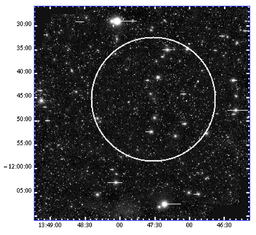
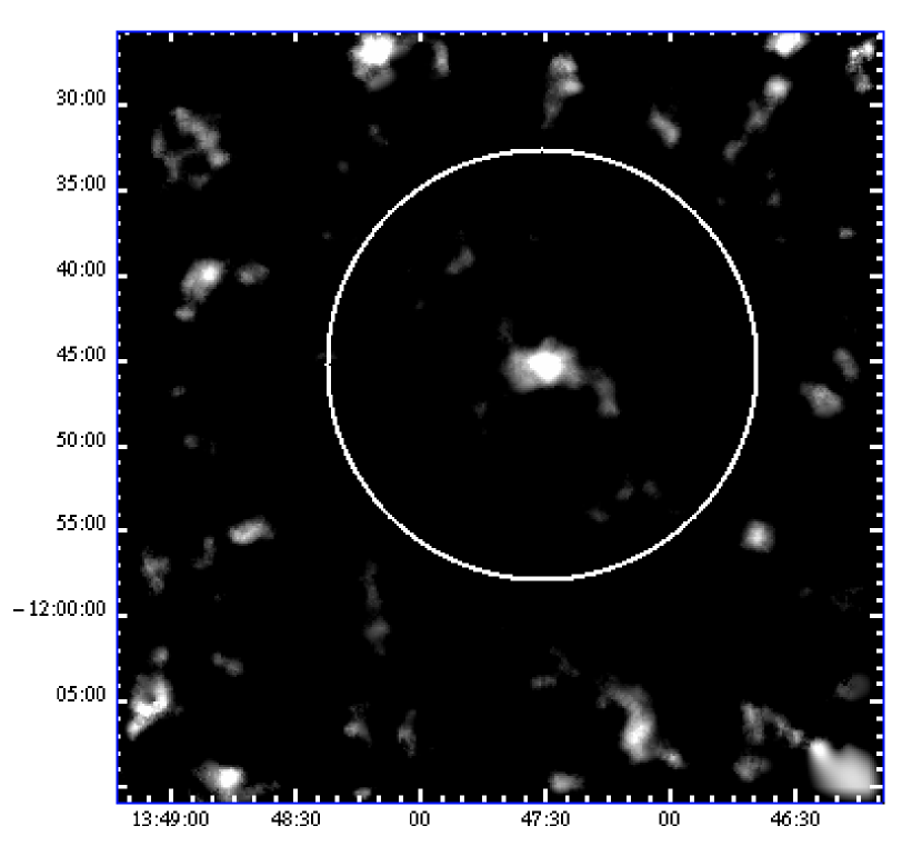
The combined band image of RXJ1347-1145 used in this study is shown in Fig. 6. The cluster is located slightly northeast of center in the frame. Figure 7 shows the two-dimensional mass map determined by the ellipticity correlations in the potential background galaxies for . This mass map has the same scale as the band image, and was produced by fiatmap, a program that determines a two-dimensional mass profile from detected correlations in object ellipticity (Wittman et al., 2002; Fischer & Tyson, 1997).
The color contrast mass map shows a strong (bright) weak lensing signal at the location of the cluster. The field appears relatively empty aside from a concentration of mass at the location of the cluster.
Using the center of the cluster determined from the mass map, we determine the average gravitational shear in radial annuli centered on the cluster. This task is accomplished by determining, for each object in a given radial annulus, the alignment of the object to a circle centered on the cluster and then averaging these values. For each annulus, we obtain an average tangential shear, , (a measure of how aligned objects are to the circle) and an estimated error in the tangential shear.
Figure 8 shows the tangential shear detected for RXJ1347–1145 with error bars from analysis of the background galaxies with . Also shown is the contribution of the residual PSF anisotropy to the tangential shear as determined by the stars. We see that the residual PSF anisotropy is consistent with zero shear detection and substantially weaker than the detection based on the potential background galaxies.
In addition to measuring average tangential shear, we can measure an average shear oriented at from tangent to the circle centered on the cluster. In weak lensing, this shear should be consistent with zero shear detection at the large radii of this study. In dashed lines, Fig. 8 shows the shear detected from the background galaxies with . That the shear is consistent with zero gives another indication that major systematic errors have been controlled.
As a third test of systematic error, we show the results of an scramble test in Fig. 9. In this test, we consider the quintuplet for the th object used in the shear detection of Fig. 8 and decouple the position from the shape information by randomly assigning shape information to positions, forming the quintuplets , where represents the same random integer for each moment.
Since weak lensing produces a position dependent shearing, the quintuplet should result in tangential shearing, but the scrambled quintuplet should not. In Fig. 9, we see that the scrambled tangential shear is consistent with zero signal.
We statistically test the null hypothesis (that the true value of is zero) by computing a statistic assuming that the error in the true value of is equal to the error in the measured . This results in a of for degrees of freedom for the sample with . The probability of obtaining a this large in the absence of a weak lensing effect is less than . The more “conservative” magnitude cut at yields for d.o.f., which corresponds to a probability of null detection less than .
For comparison, a null hypothesis test for the statistic for the shear shown in Fig. 8 results in a of for degrees of freedom, while the tangential shear measurement of the stars had a of . The scramble test yields a of for degrees of freedom, and is consistent with a null detection at .
5 Mass reconstruction
In gravitational lensing, the tangential shear, , at a given projected radius in the lens plane is related to the surface mass density, , at that radius. Defining , the ratio of the surface mass density to the critical surface density for multiple lensing, we have
| (5) |
where is the normalized, average surface mass density interior to and is the mean density at (Miralda-Escude, 1991). For a given mass model that determines , Eq. 5 allows us to relate the model parameters to the observed shear, .
The critical surface density is given by (Schneider et al., 1992)
| (6) |
where , and are the angular-diameter distances between the observer and source, observer and lens, and lens and source, respectively. Hence, is both redshift and cosmology dependent.
We will determine an average for our sample by using the known redshift of the cluster, (Cohen & Kneib, 2002), and an average value of for each the many sources.
To determine the redshifts of the sources, we develop a redshift to magnitude relation using the California Institute of Technology Faint Galaxy Redshift Survey (Cohen et al., 2000). Dividing the well measured objects in this survey into -wide magnitude bins from , we determined an initial average value of for a given magnitude. To remove outliers from each bin, we excluded objects whose measured redshift was more than one standard deviation from the bin average, and then recomputed a final average redshift for the given magnitude.
Plotting this average redshift of each bin against magnitude, and using a weighted least squares method, we determine that is related to in a linear fashion
| (7) |
where the parameters and are given by
| (8) |
The slope-intercept parameter space is degenerate, so the error bars on and from Eq. 8 are linked. Figure 10 shows the binned data from the CalTech Faint Galaxy Redshift Survey, the best fit line from Eq. 7 and two bounding curves corresponding to a confidence interval.
The Faint Galaxy Redshift Survey does not contain a sufficient number of galaxies fainter than to rule out a possible selection bias. Therefore, we posit that the linear fit found from the region of the survey will apply to our entire galaxy sample in Fig. 3, even though our sample contains objects fainter than .
We note that any error introduced in the redshift by our linear fit for objects with magnitude greater than will have a minimal impact on the eventual determination of for two reasons. First, from Fig. 4, we see that relatively few objects will be used at . Second, almost all objects this faint will lie in the vicinity of where the angular diameter distance flattens as a function of . Hence, even relatively large errors in around do not propagate strongly into errors in , or .
Applying Eq. 7 to our sample with , we determine that our sample has an average redshift, , and that the average critical surface density is pc-2 for an , cosmology with km s-1 Mpc-1. (Here, the upper and lower error limits are estimated using the bounding curves from Fig. 10.) For an , cosmology, the average is given by pc-2. For the sample with , the values for are pc-2 and pc-2 for , and , cosmologies, respectively.
In principle, the critical density varies as a function of angular radius because the magnification by the lens of background sources makes sources closer to the center of the lens appear relatively brighter than sources at a greater angular radius. This increase in brightness causes us to underestimate the redshift of the source and overestimate the critical density.
Fischer & Tyson (1997) used Monte Carlo simulations of background galaxies magnified by an isothermal lens with a velocity dispersion of km s-1 to determine a plot of versus radius. Figure 7 of their paper shows that the observed shear of their study’s innermost data points were affected by the variation in . However, accounting for this variation did not lead to a significant change in model fit, primarily because the innermost angular bins have the fewest data points and hence the highest uncertainty.
In the current wide-field study, the innermost radial bin falls over the range in which Fig. 7 of Fischer & Tyson (1997) shows a significant variation in . However, the remaining radial bins fall into a region where the variation of is within the error introduced by using the fit of Eq. 7.
Therefore, in this wide-field study, we will use a constant value of as a function of angular radius for a given cosmological model. We feel justified in doing so because the current wide-field study covers almost twice the radial size of Fischer & Tyson (1997) and hence is less susceptible to any biasing introduced by errors from the innermost data point. These errors are small because the weighted algorithms used to fit mass models discount data points with large errors.
6 Mass models
In this section, we apply two mass models to our observed shear of RXJ1347-1145: a singular isothermal sphere model (SIS) and the Navarro, Frenk, and White (NFW) model (Navarro et al., 1997). Throughout this section, we assume that the Hubble constant has a value of km s-1 Mpc-1. For each model, we consider an , cosmology, and briefly cite the best fit parameters for the , cosmology in order to compare with previous studies of this cluster. In 6.3, we summarize the cluster masses inferred from the two models.
6.1 SIS model
In the SIS model, the surface density is parameterized by the velocity dispersion, :
| (9) |
Here, is the projected radius in meters in the lens plane from the center of the cluster. In the SIS model, , so by Eq. 5, the tangential shear is related to the velocity dispersion by
| (10) |
Using a standard linear regression fitting algorithm that minimizes , we determine that the velocity dispersion predicted by our observed shear in an , cosmology is km s-1 for the magnitude cut (minimum for d.o.f.), and km s-1 for the magnitude cut (minimum for d.o.f.)
Two independent factors contribute to error in the inferred velocity dispersion. First, the process of minimizing carries with it a random statistical error that can be estimated using the argument of Press et al. (1995). We estimate that these statistical errors contribute to uncertainty in the velocity dispersion of km s-1 for a confidence interval with the cut and km s-1 for the cut. Independently, the errors bars on the lensing critical density, contribute to uncertainty in as km s-1 for and km s-1 for .
Assuming the velocity dispersion of km s-1, the SIS model corresponds to a total integrated mass of within a radius of Mpc.
For an , cosmology, the best fit velocity dispersions are km s-1 (statistical) and km s-1 (error in critical density) for and km s-1 (statistical) and km s-1 (critical density) for .
6.2 NFW model
The NFW model depends on a concentration parameter , and a scale radius . The scale radius is related to the virial radius , which is the radius inside which the mass density of the halo is equal to , where is the critical density of the universe at redshift .
From Eq. 5, we have that
| (11) |
and Wright & Brainerd (2000) derive the relevant expressions for and . Because our observational data is specified in terms of annular bins with inner and outer radii and , we must derive expressions for the average density interior to the annulus and the average density in the annulus. The average density in the annulus is given by
| (12) |
while the average density interior to the annulus is given by
| (13) |
Hence, our observed tangential shear, , for a given annulus of inner radius and outer radius is given by
| (14) |
We use Eq. 14 with the expressions for from Wright & Brainerd (2000) to determine the best fit parameters of the NFW model. As the NFW model is highly non-linear, we use the Press et al. (1995) implementation of the Levenberg-Marquardt method to fit for and , minimizing .
For an , cosmology, we find that , and Mpc, or Mpc for the cut with a minimum for thirteen d.o.f. For , we obtain , and Mpc, or Mpc with . Figure 11 shows the best fit NFW model with the observed gravitational shear for .
As for the SIS models, we estimate the statistical errors in the minimization and the error propagated from error in . In the case of the NFW models, the error in introduces a small error in the concentration parameter, for and for and less than variation in for both cuts.
Figure 12 shows the confidence region in the – plane for the cut, yielding error bars Mpc with for a NFW model in an , cosmology. The concentration parameter, is not well constrained. (The confidence region for is similar.)
We estimate error bars on the total integrated mass using the upper left and lower right projections of the confidence interval onto the – axes. The lack of constraint on yields large error bars on the total integrated mass: within and within Mpc in the , cosmology for the cut.
The best fit NFW parameters for an , cosmology are (error from ), Mpc, or Mpc with for thirteen d.o.f. for and (error from ), Mpc, or Mpc with for thirteen d.o.f. for . Again, the concentration parameter, is not well constrained by the statistical fit, as is shown in Fig. 12.
6.3 Observed Mass
Table 1 summarizes the inferred mass interior to Mpc of the cluster in SIS and NFW models for two cosmological models for the cut, while Table 2 presents the same information for the cut. We see that within a cosmological model, the NFW and SIS inferred masses generally agree within error bars, and that the choice of cosmological model makes a small difference in inferred mass. We also note that the cut generally yields a higher total integrated mass than the cut.
Figure 13 plots an observed measure of the mass densitometry of RXJ1347–1145 computed by the relation
| (15) |
introduced by Fahlman et al. (1994), where is the outer radius of the outermost annulus. Densitometry measures from SIS and NFW models in an , cosmology are shown assuming model parameters from best-fits to the gravitational shear data. The error bars are statistical error bars computed from the number of galaxies used in the calculation only.
Because the observed densitometry measure uses all of the objects between and to determine at , the values of the observed densitometry measure in Fig. 13 are not independent. In fact, small changes in values at the outer annuli give rise to large changes in the densitometry value at inner annuli, so that the actual uncertainty in the innermost annulus is quite large. Thus, although neither the SIS or NFW model fit the actual value of the innermost point, both models are adequate fits to the total profile and yield similar total integrated masses.
7 Luminosity
We present a rough estimate of the light distribution of the
cluster drawn from the band image in Fig. 14. This
estimate is limited by the difficulty of accurate background
subtraction due to the lack of a high quality image that can
be used for color selection. This luminosity estimate is also
limited by the compact nature of RXJ1347 and the relatively low
angular resolution of the central region in this study. In this
section, all measured values are the SExtractor values for
the combined band image.
We begin by selecting all non-saturated objects detected in the
band image by SExtractor with a minimal lower limit
size cut and deleting spuriously
detected objects in regions near stars. Because we can not make a
color or redshift selection, we assumed that all objects
are at the cluster redshift, and determined a total flux,
f, in radial annuli centered on the cluster. From the
total flux in each annulus, we determined a total absolute
magnitude , applying a correction of from
Fukugita et al. (1995). A luminosity relative to the solar luminosity in
each annulus was then computed from this total magnitude.
To compare this light distribution with the mass distribution determined by the weak lensing, we first determined that the luminosity per unit area is well fit by a general SIS profile. Since this is the case, we can assume that the luminosity per unit area is linearly related to the projected SIS mass density, or that
| (16) |
where the SIS model for mass density is given by the best fit parameters found from the weak lensing, or km s-1 for the , cosmology. We compute in units of solar masses per unit area and find the parameters and by minimization of
| (17) |
with
Minimizing from Eq. 17 has the advantage of finding both the approximate “background” luminosity and mass to light ratio simultaneously. Formally, the denominator of should also include a term for uncertainty in . We neglect this uncertainty because we are unable to determine its value without information about the background redshift distribution, although it is reasonable that it is approximately constant for all radial bins.
The best fit parameters, and , for seven evenly spaced annuli out to approximately Mpc are pc-2 and with for five degrees of freedom. This implies that M/ with km s-1 Mpc-1. Figure 14 plots the luminosity per unit area and best fit scaled mass density (from Eq. 16) along with scaled mass density curves.
Since we do not have error estimates on the luminosity data, we determine only the statistical uncertainty present in the fit using the argument of Press et al. (1995). This yields an error ellipse whose projections indicate that the confidence interval for the mass to light ratio is M/ .
8 Discussion
In this section, we discuss the two magnitude cuts and compare our results with the previous weak lensing results of Fischer & Tyson (1997), the recent X-ray studies of Allen et al. (2002), and the recent optical studies of Cohen & Kneib (2002). Our results indicate that there were not systematic problems in the previous weak lensing studies.
8.1 Object selection criteria
Because our imaging was poor, color selection criteria dramatically reduced the significance of our weak lensing detection by eliminating objects with well measured shapes that were undetected in the image. Thus, we were forced to employ only size and magnitude cuts to restrict our image. A size cut was used to eliminate poorly resolved objects and stars, while the magnitude cut essentially was used to control foreground objects (see Fig. 3).
In principle, it is very important to eliminate foreground and cluster objects from the catalog before analyzing gravitationally induced shears for two reasons. First, foreground objects weaken the signal because their shapes are not correlated with the weak lensing shear. Second, one might conjecture that cluster members align in some correlated way and unduly influence the gravitational shear detection if they are included.
In practice, we find that “restrictive” object selection criteria do not enhance the weak lensing detection. In this study, the conservative yielded a substantially lower total relative to the null detection (, d.o.f.) than the cut (, d.o.f.).
The magnitude cut at is reasonable based on the expected cluster magnitude of at . This cut successfully eliminates most foreground and cluster members from further analysis. This would apparently lead to a strong detection of gravitational shear by reducing the noise.
However, a cut at also eliminates a significant number of galaxies in the background of the cluster that are gravitationally lensed. The effect of removing these lensed objects from analysis weakens the signal much more than the signal is enhanced by removing the noisy foreground, and so the weak lensing detection is more significant with a less restrictive cut at the expected cluster magnitude.
We do not believe that inclusion of objects with significantly contaminates the sample or biases the weak lensing detection. In Fig. 5, we see that objects in the innermost radial bins are slightly brighter than in the outer bins. However, if we consider the over-density of objects with in the “cluster” region interior to an angular radius of , we estimate that less than additional objects have been added to the catalog of over total objects with .
Further, we observe that the mass inferred from the best fit parameters of SIS and NFW models for the sample of objects with is only slightly higher than that from objects with . In fact, the statistical error bars have significant overlap for the two magnitude cuts.
We believe that the results from the magnitude cut represent a better measurement of weak gravitational lensing than the magnitude cuts because the significance of detection is much higher. However, the best fit model parameters are similar, and the basic conclusions of the paper are unchanged for either magnitude cut.
8.2 Previous weak lensing observation
The general results of this paper are in agreement with the results of Fischer & Tyson (1997), who report that the total integrated mass within Mpc is , and that the velocity dispersion is km s-1 for SIS model assuming an isotropic velocity dispersion and an cosmology. These values are consistent with our results for the same model.
As is seen in Fig. 9, the wide-field weak lensing observations presented here confirm the detection of Fischer & Tyson (1997), which was limited to an approximately radius. The current wide-field study continues to detect significant gravitational shear at ; however, the impact this shear has on the model parameters in SIS and NFW models is minimal.
The mass to light ratio of the cluster measured in this study agrees relatively well with Fischer & Tyson (1997), who find values of M/LR M. This is quite remarkable considering the difference in methods and difficulty of background subtraction in the current study.
That the current weak lensing study obtains results in agreement with the results of Fischer & Tyson (1997) gives a strong indication that the concerns regarding the use of smaller images in determining properties from lensing studies were unfounded. The large field of view of this study and extremely robust weak lensing detection strongly confirms the results of Fischer & Tyson (1997).
8.3 Recent X-ray observations
Our results are also in good agreement with the recent Chandra X-ray observations of Allen et al. (2002). Using an NFW model, Allen et al. (2002) determine a best-fit scale radius of Mpc with a concentration parameter of . These values correspond to a virial radius Mpc and an integrated mass within the virial radius of .
The current weak lensing observations find a similar virial radius, Mpc, and a consistent mass for the same cosmological model. Figure 12 shows the confidence region for the best fit parameters and for the current weak lensing study with and the location of the parameters found by Allen et al. (2002). The recent Chandra results are also consistent with a magnitude cut.
Allen et al. (2002) report that a SIS model does not provide a good fit to the Chandra observations. Our observations are more tolerant of a SIS model because we do not have lensing observations close to the center of the cluster, a region that is well sampled and integral for the X-ray study’s conclusions.
8.4 Recent spectroscopic observations
This weak lensing study is not consistent with the results of the most recent optical velocity dispersion study by Cohen & Kneib (2002). Cohen & Kneib (2002) report a velocity dispersion of km s-1, corresponding to an integrated mass of within Mpc. This predicted mass is approximately of the mass estimated by the current weak lensing observations, and is inconsistent with our results at the level.
Cohen & Kneib (2002) suggest that their results may be artificially low if RXJ1347-1145 consists of two clusters caught in the act of merging in a direction perpendicular to the line of sight. This flow would have a minimal effect on the wide-field lensing signal analyzed in this study because the wide-field imaging does not have sufficient resolution to examine the interior region of the cluster.
9 Conclusions
In conclusion, the findings of this paper confirm the earlier weak lensing study of Fischer & Tyson (1997) and are consistent with the recent X- ray observations of Allen et al. (2002) and Ettori et al. (2001). From these findings, we conclude that there were no substantial systematic errors introduced in the older lensing study of this system by Fischer & Tyson (1997) through the relatively small field of view. Confirming the older weak lensing observations of Fischer & Tyson (1997) using a wide-field observation gives substantial evidence that weak lensing may not be significantly biased by relatively small fields of view.
This study’s results are in substantial disagreement with the direct optical velocity dispersion measurements of Cohen & Kneib (2002). As the X-ray and lensing results now tend to cluster around a velocity dispersion of approximately km s-1, it is unlikely that the km s-1 measurement of Cohen and Kneib is correct. Cohen & Kneib (2002), recognizing this difference suggest that a possible merger within the cluster perpendicular to the line of sight could account for the observed difference.
In the current study, we did not attempt to measure weak lensing signals interior to the two arc candidates located approximately from the center of the cluster. Because the original goal of this study was to test the small field of view of Fischer & Tyson (1997), the wide-field image used in this study does not have enough resolution or depth to conclusively measure weak lensing signals in the central region of the RXJ1347-1145.
For this reason, we can not attempt to locate substructure within the cluster to test Cohen and Kneib’s assertion in this study or compare our results to recent strong lensing observations. In addition, we suspect that it is the X-ray observation’s greater sensitivity to the central region of RXJ1347-1145 that accounts for the inability of Allen et al. (2002) to find a good SIS fit.
Future high resolution lensing studies of the interior region of RXJ1347-1145 may yield interesting results. We note that the two-dimensional mass map presented in Fig. 7 does suggest some structure, leading to the hope that high resolution weak lensing studies of the central region may shed light on possibility of a significant merging event.
References
- Allen et al. (2002) Allen, S.W., Schmidt, R.W., & Fabian, A.C., 2002, MNRAS, 335, 256A
- Allen & Fabian (1998) Allen, S.W. & Fabian, A.C., 1998, MNRAS, 297, L57
- Bernstein & Jarvis (2002) Bernstein, G.M. & Jarvis, M., 2002, AJ, 123, 583B
- Bertin & Arnouts (1996) Bertin, E. & Arnouts, S., 1996, A&A Sup Ser 117, 393
- Cohen et al. (2000) Cohen, J.G. et al., 2000, ApJ, 538, 1
- Cohen & Kneib (2002) Cohen, J.G. & Kneib, J.P., 2002, ApJ, 513, 524C
- Ettori et al. (2001) Ettori. S., Allen, S.W., & Fabian, A.C., 2001 MNRAS, 322, 187
- Fahlman et al. (1994) Falman, G.G. et al., 1994 ApJ, 436, 56
- Fischer & Tyson (1997) Fischer, P., Tyson, J.A., 1997, AJ, 114 14
- Fukugita et al. (1995) Fukugita et al., 1995 PASP, 107, 945
- Komatsu et al. (2001) Komatsu, E. et al., 2001, PASJ, 53, 57
- Khiabanian (2003) Khiabanian, H. personal communication
- Miralda-Escude (1991) Miralda-Escude, J., 1991, ApJ, 370, 1
- Navarro et al. (1997) Navarro, J. F., Frenk, C. S. & White, S. D.M., 1997, ApJ490, 493
- Pointecouteau et al. (2001) Pointecouteau, E., Giard, M., Benoi, A., Desert, F.X., Bernard, J.P., Coron, N. & Lamarre, J.M., 2001, ApJ, 552, 42
- Press et al. (1995) Press, W.H. et al., 1995, Numerical Recipes, Cambridge University Press
- Schindler et al. (1995) Schindler, S. et al., 1995, A&A, 299L, 9
- Schindler et al. (1997) Schindler, S., Hattori, M., Neumann, D.M. & Böhringer, H., 1997 A&A, 317, 646
- Schneider et al. (1992) Schneider, P., Ehlers, J. & Falco, E.E., 1992, Gravitational Lensing, Springer-Verlag
- Shectman et al. (1996) Shectman, S.A. et al., 1996 ApJ, 470, 172s
- Wittman et al. (2002) Wittman, D.E., et al., 2002, SPIE, 4836, p. 21
- Wright & Brainerd (2000) Wright, C.O. & Brainerd, T.G., 2000, ApJ, 534, 34W
| Model | Cosmology | Parameters | Mass ( Mpc) |
|---|---|---|---|
| SIS | , | km s-1 | |
| SIS | , | km s-1 | |
| NFW | , | ||
| Mpc | |||
| NFW | , | ||
| Mpc |
| Model | Cosmology | Parameters | Mass ( Mpc) |
|---|---|---|---|
| SIS | , | km s-1 | |
| SIS | , | km s-1 | |
| NFW | , | ||
| Mpc | |||
| NFW | , | ||
| Mpc |