Diffusive Synchrotron Radiation from Relativistic Shocks in Gamma-Ray Burst Sources

Abstract

The spectrum of electromagnetic emission generated by relativistic electrons scattered on small-scale random magnetic fields, implied by current models of the magnetic field generation in the gamma-ray burst sources, is considered. The theory developed includes both perturbative and non-perturbative versions and, therefore, suggests a general treatment of the radiation in arbitrary small-scale random field. It is shown that a general treatment of the random nature of the small-scale magnetic field, as well as angular diffusion of the electrons due to multiple scattering by magnetic inhomogeneities (i.e., non-perturbative effects), give rise to a radiation spectrum that differs significantly from so-called “jitter” spectrum. The spectrum of diffusive synchrotron radiation seems to be consistent with the low energy spectral index distribution of the gamma-ray bursts.

1 Introduction

Relativistic objects including, but not limited to, Gamma-Ray Burst (GRB) sources are known to produce nonthermal emission, which typically requires the generation of extra magnetic field, at least at some stage of ejecta expansion after initial prompt energy release (Mészáros, 2002). A number of recent publications (Kazimura et al., 1998; Medvedev & Loeb, 1999; Nishikawa et al., 2003; Jaroshek et al., 2004, 2005) put forward the concept of magnetic field generation by a relativistic version of the Weibel instability (Weibel, 1959). Analytical considerations (Medvedev & Loeb, 1999), together with more sophisticated numerical modelling (Nishikawa et al., 2003, 2005; Jaroshek et al., 2004, 2005; Hededal & Nishikawa, 2005), suggest that the magnetic field produced by the Weibel instability is random and extremely small-scale, with a characteristic correlation length $l_{cor}\sim(0.1-1)l_{sk}$, where $l_{sk}=c/\omega_{pe}$ is the plasma skin depth, $\omega_{pe}$ is the electron plasma frequency, and $c$ is the speed of light.

Depending on the magnetic field saturation value $B$, this correlation length may be less than the coherence length (or formation zone) of synchrotron radiation:

$$l_{s}=\frac{mc^{2}}{eB}=\frac{c}{\omega_{Be}}.$$ (1)

Here, $e$ and $m$ are the electron charge and mass, and $\omega_{Be}=\frac{eB}{mc}$ is the electron gyrofrequency. Generation of electromagnetic emission by relativistic electrons moving in small-scale magnetic fields is known to differ from the case of emission by electrons in a uniform (large-scale) magnetic field (Landau & Lifshitz, 1971).

Electromagnetic radiation in small-scale random magnetic fields was first calculated by Nikolaev & Tsytovich (1979) using perturbation theory, where the trajectory of the particle is assumed to be rectilinear, while the acceleration produced by the random variations of the Lorentz force is taken into account by the first non-zero order of the perturbation theory. The full non-perturbative theory was later worked out by Toptygin & Fleishman (1987a); Toptygin et al. (1987), allowing in particular net deflections of the radiating particles that are not necessarily small (e.g., by a large-scale magnetic field and/or multiple scattering on small-scale inhomogeneities).

Recently, interest in this emission process in the context of gamma-ray bursts was revived by Medvedev (2000), who estimated radiation spectrum in the presence of the small-scale magnetic field and referred to the resulting radiation as “jitter radiation”. An oversimplification of the estimates performed by Medvedev (2000) resulted in the low-frequency asymptotic limit of the jitter spectrum, $P(\omega)\propto\omega$, which is applicable to a simpler (undulator-like) version of what is considered here, while may noticeably deviate from the correct spectral shape in a general case. In this paper a general treatment of the radiation produced by relativistic electrons moving through small-scale fluctuating magnetic fields, probably available at the relativistic shocks, is presented. For the completeness and convenience of further applications, we first formulate a simplified perturbative version of the theory, and then specify its region of applicability by comparing with the available non-perturbative version. Possible implications of the general theory for GRB physics are discussed.

2 Perturbation theory of diffusive synchrotron radiation

Let us calculate the radiation by a single relativistic particle moving in a random small-scale magnetic field based on the equation for the radiated energy resulting from perturbation theory (Landau & Lifshitz, 1971)

$$\frac{dW_{\omega}}{d\omega}=\frac{2\pi e^{2}}{c^{3}}\int_{1/2\gamma_{*}^{2}}^{\infty}\left(\frac{\omega}{\omega^{\prime}}\right)^{2}\left|{\bf w}_{\omega^{\prime}\bot}\right|^{2}\left[1-\frac{\omega}{\omega^{\prime}\gamma_{*}^{2}}+\frac{\omega^{2}}{2\omega^{\prime 2}\gamma_{*}^{4}}\right]d\left(\frac{\omega^{\prime}}{\omega}\right).$$ (2)

Here $\gamma_{*}=\gamma=E/mc^{2}$ in the vacuum, while $\gamma_{*}^{-2}=\left(\gamma^{-2}+\frac{\omega_{pe}^{2}}{\omega^{2}}\right)$ in the presence of the background plasma, $\omega^{\prime}=\frac{\omega}{2}(\gamma^{-2}+\theta^{2}+\omega_{pe}^{2}/\omega^{2})$, $\theta$ is the angle between the electron speed and the direction of the emission, ${\bf w}_{\omega^{\prime}\bot}$ is the Fourier transform of the particle acceleration ${\bf w}_{\bot}={\bf F}/(m\gamma)$ transverse to the particle speed, and ${\bf F}$ is the corresponding transverse component of the Lorentz force. Evidently, for a random Lorentz force the acceleration is a random function as well, although the average of $\left|{\bf w}_{\omega^{\prime}\bot}\right|^{2}$ includes a regular (not random) component, which eventually specifies the emission pattern.

To find the averaged value of $\left|{\bf w}_{\omega^{\prime}\bot}\right|^{2}$, assume that the random Lorentz force (${\bf F}({\bf r},t)$, which can include either magnetic and/or electric fields) perturbing the rectilinear particle motion, can be expressed as a Fourier integral over $\omega$ and ${\bf k}$:

$${\bf F}({\bf r},t)=\int e^{-i(\omega t-{\bf kr})}{\bf F}_{\omega,{\bf k}}d\omega d{\bf k}.$$ (3)

This force represents a global field, which can vary in space and time in general. However, the particle acceleration is produced by a local value of this field related to instantaneous positions of the particle along its actual trajectory. Within the perturbation theory we can adopt ${\bf r}={\bf r}_{0}+{\bf v}t$ for the independent argument of the force acting on the moving particle:

$${\bf F}({\bf r}_{0}+{\bf v}t,t)=\int e^{-i(\omega t-{\bf kr}_{0}-{\bf kv}t)}{\bf F}_{\omega,{\bf k}}d\omega d{\bf k}.$$ (4)

Then the Fourier component ${\bf F}_{\omega^{\prime}}$, specifying the magnitude ${\bf w}_{\omega^{\prime}}={\bf F}_{\omega^{\prime}}/{m\gamma}$, can be found by direct temporal Fourier transform of (4):

$${\bf F}_{\omega^{\prime}}=\int\frac{dt}{2\pi}e^{i\omega^{\prime}t}{\bf F}({\bf r}_{0}+{\bf v}t,t)=\int d\omega d{\bf k}\delta(\omega^{\prime}-\omega+{\bf kv}){\bf F}_{\omega,{\bf k}}e^{i{\bf kr}_{0}}.$$ (5)

Now it is straightforward to write down the square of the force modulus $\mid{\bf F}_{\omega^{\prime}}\mid^{2}$:

$$\mid{\bf F}_{\omega^{\prime}}\mid^{2}=\int d\omega d{\bf k}d\omega_{1}d{\bf k}_{1}e^{i({\bf k}-{\bf k}_{1}){\bf r}_{0}}\delta(\omega^{\prime}-\omega+{\bf kv})\delta(\omega^{\prime}-\omega_{1}+{\bf k}_{1}{\bf v}){\bf F}_{\omega,{\bf k}}{\bf F}_{\omega_{1},{\bf k}_{1}}^{*}.$$ (6)

This value is still fluctuating in the random field, although its mean value is non-zero (in contrast to the fluctuating field itself ${\bf F}_{\omega,{\bf k}}$, which is a complex random function with zero mean). A steady-state level of radiation is evidently specified by the average value $\left<\mid{\bf F}_{\omega^{\prime}}\mid^{2}\right>$ of (6). The easiest way to perform the averaging is to average Eq. (6) over all possible initial positions ${\bf r}_{0}$ of the particle inside the source. In practice, this corresponds to a uniform distribution of radiating particles within a volume containing the field inhomogeneities, which have a statistically uniform distribution within the same volume. Since the exponent $\exp({i({\bf k}-{\bf k}_{1}){\bf r}_{0}})$ oscillates strongly for ${\bf k}\neq{\bf k}_{1}$, we obtain:

$$\frac{1}{V}\int e^{i({\bf k}-{\bf k}_{1}){\bf r}_{0}}d{\bf r}_{0}=\frac{(2\pi)^{3}}{V}\delta({\bf k}-{\bf k}_{1}),$$ (7)

where $V$ is the source volume, and, for $\left<\mid{\bf F}_{\omega^{\prime}}\mid^{2}\right>$ obtain accordingly

$$\left<\mid{\bf F}_{\omega^{\prime}}\mid^{2}\right>=\frac{(2\pi)^{3}}{V}\int d\omega d{\bf k}\delta(\omega^{\prime}-\omega+{\bf kv})\mid{\bf F}_{\omega,{\bf k}}\mid^{2}.$$ (8)

Then the mean value of the Fourier transform of the particle acceleration is expressed as

$$\mid{\bf w}_{\omega^{\prime}\bot}\mid^{2}=\frac{(2\pi)^{3}}{m^{2}\gamma^{2}V}\int d\omega d{\bf k}\delta(\omega^{\prime}-\omega+{\bf kv})\mid{\bf F}_{\omega,{\bf k}}\mid^{2},$$ (9)

which provides a unique correspondence between the temporal and spatial Fourier transform of the Lorentz force (right-hand side) and the temporal Fourier transform of the particle acceleration (left-hand side). Substituting (9) into (2), using dummy variables ($q_{0},{\bf q}$) for ($\omega,{\bf k}$), we obtain finally for the radiated energy per unit range of $\omega$

$$\frac{dW_{\omega}}{d\omega}=\frac{(2\pi)^{4}e^{2}}{m^{2}c^{3}\gamma^{2}V}\int_{1/2\gamma_{*}^{2}}^{\infty}d\left(\frac{\omega^{\prime}}{\omega}\right)\left(\frac{\omega}{\omega^{\prime}}\right)^{2}\left[1-\frac{\omega}{\omega^{\prime}\gamma_{*}^{2}}+\frac{\omega^{2}}{2\omega^{\prime 2}\gamma_{*}^{4}}\right]\int dq_{0}d{\bf q}\delta(\omega^{\prime}-q_{0}+{\bf qv})\mid{\bf F}_{q_{0},{\bf q}}\mid^{2}.$$ (10)

The spectrum of the radiation described by Eq. (10) depends on the statistical properties of the random force. To be more specific let us consider a random magnetic field, i.e., $\mid{\bf F}_{q_{0},{\bf q}}\mid^{2}=e^{2}\mid{\bf B}^{\bot}_{q_{0},{\bf q}}\mid^{2}=e^{2}(\delta_{\alpha\beta}-v_{\alpha}v_{\beta}/v^{2})B^{\alpha}_{q_{0},{\bf q}}B^{\beta*}_{q_{0},{\bf q}}$, and introduce the second-order correlation tensor of the statistically uniform random magnetic field as follows (Toptygin, 1985):

$$K_{\alpha\beta}^{(2)}({\bf r},\tau)=\left<B_{st,\alpha}({\bf R},t)B_{st,\beta}({\bf R}+{\bf r},t+\tau)\right>=\frac{1}{TV}\int dtd{\bf R}B_{st,\alpha}({\bf R},t)B_{st,\beta}({\bf R}+{\bf r},t+\tau).$$ (11)

Then, express $\mid{\bf B}^{\bot}_{q_{0},{\bf q}}\mid^{2}$ via the Fourier spectrum $K_{\alpha\beta}^{(2)}(q_{0},{\bf q})$ of this correlation tensor:

$$\mid{\bf B}^{\bot}_{q_{0},{\bf q}}\mid^{2}=\frac{TV}{(2\pi)^{4}}\left(\delta_{\alpha\beta}-\frac{v_{\alpha}v_{\beta}}{v^{2}}\right)K_{\alpha\beta}^{(2)}(q_{0},{\bf q})=\frac{TV}{(2\pi)^{4}}K(q_{0},{\bf q})$$ (12)

where $K(q_{0},{\bf q})=K_{\alpha\beta}^{(2)}(q_{0},{\bf q})\left(\delta_{\alpha\beta}-\frac{v_{\alpha}v_{\beta}}{v^{2}}\right)$ is the spectrum of the random magnetic field transverse to the particle velocity. If the random field is composed of random waves with the dispersion relation $q_{0}=q_{0}({\bf q})$ (in the limiting case of a static random field we have $q_{0}({\bf q})\equiv 0$), the spectrum takes the form $K(q_{0},{\bf q})=K({\bf q})\delta(q_{0}-q_{0}({\bf q}))$.

Substituting all required values into (9) and dividing by the total duration of emission $T$ we arrive at the radiation intensity (energy emitted per unit frequency per unit time):

$$\frac{dI_{\omega}}{d\omega}=\frac{e^{4}}{m^{2}c^{3}\gamma^{2}}\int_{1/2\gamma_{*}^{2}}^{\infty}d\left(\frac{\omega^{\prime}}{\omega}\right)\left(\frac{\omega}{\omega^{\prime}}\right)^{2}\left[1-\frac{\omega}{\omega^{\prime}\gamma_{*}^{2}}+\frac{\omega^{2}}{2\omega^{\prime 2}\gamma_{*}^{4}}\right]\int dq_{0}d{\bf q}\delta(\omega^{\prime}-q_{0}+{\bf qv})K({\bf q})\delta(q_{0}-q_{0}({\bf q})),$$ (13)

which eventually results in radiation spectra different from one estimated by Medvedev (2000).

3 Illustrative examples

It is now straightforward to consider a few different models of the random magnetic field. Let us proceed with the case of quasi-static magnetic inhomogeneities, $K_{\alpha\beta}^{(2)}(q_{0},{\bf q})=K_{\alpha\beta}^{(2)}({\bf q})\delta(q_{0})$, which is applicable for magnetic inhomogeneities moving slower than the radiating particle. In the general case we assume:

$$K_{\alpha\beta}^{(2)}({\bf q})=C_{\alpha\beta}\left<B_{st}^{2}\right>f({\bf q}),$$ (14)

where the tensor structure of $C_{\alpha\beta}$ should be consistent with Maxwell’s Equation $\nabla\cdot{\bf B}=0$ and provide the correct normalization $\int K_{\alpha\alpha}^{(2)}({\bf q})d{\bf q}=\left<B_{st}^{2}\right>$.

Consider the isotropic case $K_{\alpha\beta}^{(2)}({\bf q})\propto\left(\delta_{\alpha\beta}-q_{\alpha}q_{\beta}/q^{2}\right)f(\mid{\bf q}\mid)$ with a specific power-law for the spectrum of random magnetic field:

$$f({\bf q})=\frac{q^{2}}{(q_{m}^{2}+q^{2})^{\nu/2+2}},$$ (15)

where $\nu$ is the high-frequency spectral index of the magnetic turbulence. The integral over $d{\bf q}$ then takes the form:

$$\int d{\bf q}\frac{q^{2}\delta(\omega^{\prime}+{\bf qv})}{(q_{m}^{2}+q^{2})^{\nu/2+2}}=\frac{2\pi}{v}\left[\frac{1}{\nu}\left(\left(\frac{\omega^{\prime}}{v}\right)^{2}+q_{m}^{2}\right)^{-\nu/2}-\frac{q_{m}^{2}}{\nu+2}\left(\left(\frac{\omega^{\prime}}{v}\right)^{2}+q_{m}^{2}\right)^{-\nu/2-1}\right].$$ (16)

Subsequent integration over $d(\omega^{\prime}/\omega)$ yields the radiation spectrum over the entire spectral range. We consider the low-frequency and high-frequency asymptotic behavior of the spectrum. At high frequencies, $\omega\gg\omega_{0}\gamma^{2}$, where $\omega_{0}=q_{m}c$, $q_{m}$ can be discarded everywhere in Eq. (16), so after integration over $d(\omega^{\prime}/\omega)$ we have $dI_{\omega}/d\omega\propto\omega^{-\nu}$ and the radiation spectrum resembles the turbulence spectrum at $q\gg q_{m}$. At low frequencies, $\omega\ll\omega_{0}\gamma^{2}$, the term $\omega^{\prime}/v$ can be discarded in (16), which leads to the frequency-independent part of the spectrum $dI_{\omega}/d\omega\propto\omega^{0}$. At even lower frequencies, $\omega<\omega_{pe}\gamma$, when the difference between $\gamma$ and $\gamma_{*}$ is important, the term $\omega^{\prime}/v$ dominates again giving rise to the spectral asymptote $dI_{\omega}/d\omega\propto\omega^{2}$.

Note that this property does not depend on the specific shape of the correlation function $f({\bf q})$ in the range of small $q\ll q_{m}$ ($\propto q^{2}$ in our case), and remains valid for any shape peaking at $q_{m}$. To see this explicitly, consider the following simplified form of the spectrum: $f({\bf q})\propto q^{\alpha}$ at $q<q_{m}$ and $f({\bf q})=0$ at $q>q_{m}$. Therefore, in place of (16) we have:

$$\int d{\bf q}q^{\alpha}\delta(\omega^{\prime}+{\bf qv})=\frac{2\pi}{(\alpha+2)v}\left[q_{m}^{\alpha+2}-\left(\frac{\omega^{\prime}}{v}\right)^{\alpha+2}\right],$$ (17)

which does not depend on $\omega$ at $\omega^{\prime}\ll\omega_{0}$ (or $\omega\ll\omega_{0}\gamma^{2}$) for $\alpha>-2$, thus, for any fluctuation energy spectrum, $q^{2}f({\bf q})$, peaking at $q_{m}$. In particular, this is also valid for the Bremsstrahlung spectrum, which arises as the fast particle experiences random accelerations at microscopic scales by randomly distributed Coulomb centers.

We now demonstrate that the same is valid for the two-dimensional geometry implied by the current models of magnetic field generation at the relativistic shocks (Medvedev & Loeb, 1999; Nishikawa et al., 2003; Jaroshek et al., 2004, 2005). Consider a specific case, when the observer looks along the $x$ axis, the shock front lies in the $xy$ plane, and the random field belongs to the shock front, first examined by Medvedev (2000), who obtained a result different from one given below. Note, that now the most general form of $K_{\alpha\beta}({\bf q})$ is

$$K_{\alpha\beta}^{(2)}({\bf q})\propto\left(\delta_{\alpha\beta}-n_{\alpha}n_{\beta}\right)f(q_{z},q_{x}^{2}+q_{y}^{2}),$$ (18)

where ${\bf n}$ is the unit vector normal to the shock front. Since we observe along the $x$ axis, particles moving along this direction are the main contributors to the emission, so that ${\bf qv}=q_{x}v$ in the argument of $\delta$-function. Thus, we obtain:

$$\int d{\bf q}\delta(\omega^{\prime}+q_{x}v)f({\bf q})=\frac{1}{v}\int dq_{y}\bar{f}(q_{y}^{2}+(\omega^{\prime}/v)^{2}),$$ (19)

where $\bar{f}(q_{x}^{2}+q_{y}^{2})=\int f({\bf q})dq_{z}$. The correlation function $f({\bf q})$ has a peak around $q_{m}=2\pi/l_{cor}$. Assuming the function $\bar{f}$ keeps this property, which is typically the case, then at small frequencies ($\omega^{\prime}\ll\omega_{0}$) integral (19) does not depend on frequency, and the substitution of it into (13) gives rise to a frequency-independent spectrum $dI_{\omega}/d\omega\propto\omega^{0}$, which is flatter (not steeper) than the asymptotic spectrum of synchrotron radiation.

Thus, this flat low-frequency spectrum seems to be rather common in the presence of small-scale random magnetic or electric fields. However, in some specific models of the random field, the low-frequency spectrum can deviate from the flat spectrum.

As an example of this latter point, consider a (somewhat artificial) factorized correlation function $f({\bf q})=f_{1}(q_{\|})f_{2}({\bf q}_{\bot})$, where $q_{\|}$ and ${\bf q}_{\bot}$ stand for components parallel and transverse to the particle velocity (note that a special model of the field, which is uniform in the plane transverse to the particle velocity, when $f({\bf q})=f_{1}(q_{\|})\delta({\bf q}_{\bot})$, is absorbed by this particular case). Then, integrations over $dq_{\|}$ and $d{\bf q}_{\bot}$ can be performed independently, so that

$$\int d{\bf q}\delta(\omega^{\prime}+q_{\|}v)f({\bf q})=\frac{1}{v}f_{1}(\omega^{\prime}/v)\int d{\bf q}_{\bot}f_{2}({\bf q}_{\bot}),$$ (20)

and the low-frequency asymptote of the radiation spectrum is ultimately specified by the behavior of $f_{1}(q_{\|})$ at $q_{\|}\ll q_{m}$ (e.g., $f_{1}(\omega^{\prime}/v)\propto(\omega^{\prime}/v)^{2}$ for correlation function like (15)), and can easily be steeper than $\omega^{0}$ spectrum with the steepest possible asymptote $\omega^{1}$ (ignoring non-perturbative effects and wave dispersion).

To see this, consider an extreme case of a small-scale field, namely, one comprising a single spatial harmonic $f({\bf q})=\delta({\bf q}-{\bf q}_{m})$, which evidently provides the narrowest possible radiation spectrum. All integrations are extremely easy in this case, in particular,

$$\int d{\bf q}\delta(\omega^{\prime}+{\bf qv})\delta({\bf q}-{\bf q}_{m})=\delta(\omega^{\prime}+{\bf q}_{m}{\bf v}),$$ (21)

giving rise to the linear low-frequency asymptote $dI_{\omega}/d\omega\propto\omega^{1}$, in agreement with the estimate of Medvedev (2000). A similar kind of regular (but small-scale) acceleration takes place in undulators or in the case of so-called small-pitch-angle radiation (Epstein, 1973; Epstein & Petrosian, 1973), resulting in a similar radiation spectrum. However, in the general case of a stochastic magnetic field, the radiation spectrum deviates strongly from this simpler case.

4 Non-perturbative approach

It should be emphasized, that the applicability of the perturbation theory developed above is itself rather limited. Indeed, even if the deflection of the particle is small during the time needed to pass through a single correlation cell of the random field, it is not necessarily small along the coherence length of the emission, since multiple scattering of the particle by several successive magnetic inhomogeneities can easily provide large enough deflections due to angular diffusion to render perturbation theory inapplicable.

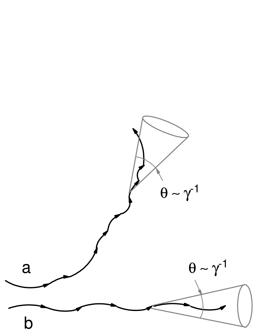
Figure 1: Random walk of the particle in the random field (a) vs jitter in small-scale regular field (b). In the former case the mean square of the deflection angle $\theta_{c}$ increases with time as $\theta_{c}^{2}\propto t$, while in the later case it remains small along the entire trajectory. As a result, the radiation spectra deviate strongly from each other for these two cases.

Thus, we explicitly have to consider the applicability of perturbation theory to the emission of fast particles moving in the small-scale random fields. The coherence length $l_{c}(\omega)\sim c\gamma_{*}^{2}/\omega$ of emission by relativistic particle with the Lorentz-factor $\gamma$ at a frequency $\omega$ decreases as frequency increases, so the approximation of the rectilinear motion is eventually valid at sufficiently large frequencies. However, at lower frequencies the coherence length may be larger than the correlation length of the random field, and this necessarily will be the case at low enough frequencies if one neglects the effect of the wave dispersion in the plasma. Thus, the particle trajectory traverses several correlation lengths of the random field to emit this low frequency, and its trajectory random walks due to uncorrelated scattering by successive magnetic inhomogeneities, as depicted in fig. 1. This angular diffusion will clearly affect the radiation spectrum if the mean angle of the particle deflection $\theta_{c}$ accumulated along the coherence length $l_{c}$ exceeds the beaming angle of the emission $\gamma^{-1}$.

To estimate the deflection angle $\theta_{c}$, adopt that the random field consists of cells with the characteristic scale $l_{0}$ and rms field value $\left<B_{st}^{2}\right>^{1/2}$. Inside each cell, the electron velocity rotates by the angle $\theta_{0}\sim(\omega_{st}/\gamma)(l_{0}/c)\sim\omega_{st}/(\omega_{0}\gamma)$, where $\omega_{st}=e\left<B_{st}^{2}\right>^{1/2}/mc$ and $\omega_{0}=2\pi c/l_{0}$. Since the deflections are produced by successive uncorrelated cells of the random field, the mean square of the deflection angle after traversing $N$ cells will be $\theta_{c}^{2}=\theta_{0}^{2}N$, where the number of the cells is specified by the ratio of the coherence length $l_{c}$ to the correlation length $l_{0}$ of the random field, $N=l_{c}/l_{0}$. Therefore, when the particle passes the length $l_{c}(\omega)$ required to produce the emission at a frequency $\omega$, its characteristic deflection angle is $\theta_{c}^{2}\simeq\omega_{st}^{2}/(\omega_{0}\omega)$. This angular diffusion will strongly affect the emission if $\theta_{c}\ \raise 3.0pt\hbox{$>$}\kern-8.5pt\raise-2.0pt\hbox{$\sim$}\ 1/\gamma$, i.e., at

$$\omega\ \raise 3.0pt\hbox{$<$}\kern-8.5pt\raise-2.0pt\hbox{$\sim$}\ \frac{\omega_{st}^{2}}{\omega_{0}}\gamma^{2},$$ (22)

which occurs in the range of the low-frequency asymptotic limit discussed above.

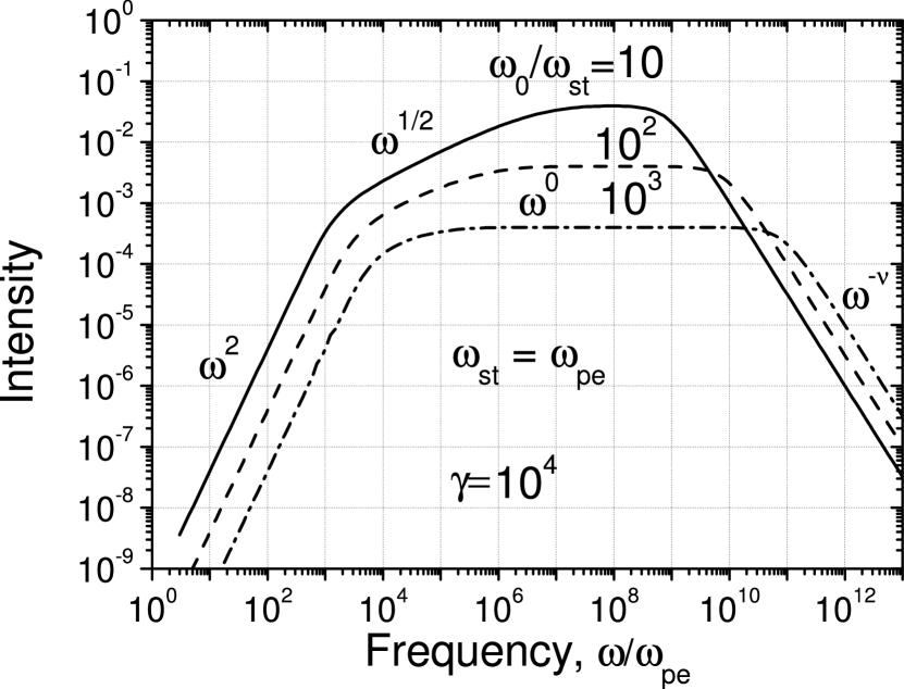
Figure 2: Radiation spectra produced by a relativistic particle with $\gamma=10^{4}$ in a small-scale random magnetic field. The spectral asymptote $\omega^{1/2}$ can only be obtained within the non-perturbative theory. If $\omega_{0}$ is large enough (e.g., $\omega_{0}/\omega_{st}=10^{3}$ in the figure) the spectral region provided by multiple scattering, $\omega^{1/2}$, disappears, and the whole spectrum is the same as within the perturbation theory.

The non-perturbative version of the theory is not discussed in any detail here since it is published elsewhere (Toptygin & Fleishman, 1987a, b; Toptygin et al., 1987; Fleishman, 2006). The full radiation spectrum (also including the effect of a regular magnetic field, if present) is given by Eq. (35) of (Toptygin & Fleishman, 1987a). Fig. 2 presents radiation spectra (calculated with the use of the non-perturbative formulae (35) of (Toptygin & Fleishman, 1987a), or, equivalently, Eq. (30) of (Fleishman, 2006)) for a single relativistic electron with a Lorentz-factor $\gamma=10^{4}$ moving in the presence of fluctuating small-scale fields (with different ratios $\omega_{st}/\omega_{0}=10^{-1},10^{-2},10^{-3}$, the regular magnetic field is assumed to be very weak, the distribution of random field is isotropic (like (15)), and $\omega_{pe}=\omega_{st}$. Although the combination of parameters adopted to produce Fig. 2 does not span all the regimes possibly relevant to the GRB case (see also the review paper Fleishman (2006)), it shows the variety of asymptotes in one plot and displays spectra both affected and unaffected by the non-perturbative effects, which should be sufficient for illustration purpose.

The solid curve corresponds to the parameters similar to those adopted by Medvedev (2000) for the GRB sources ($\omega_{0}=10\omega_{st}=10\omega_{pe}$). Although the flat region obtained already within the perturbation approach exists, it is easy to see a region of the radiation spectrum $dI_{\omega}/d\omega\propto\omega^{1/2}$, provided by the multiple scattering, which occupies the frequency range

$$\omega_{pe}(\omega_{pe}\omega_{0}\gamma^{2}/\omega_{st}^{2})^{1/3}\ll\omega\ll\frac{\omega_{st}^{2}}{\omega_{0}}\gamma^{2}.$$ (23)

Note, that the left bound of this inequality is below the limit $\omega_{pe}\gamma$ imposed by the effect of the wave dispersion in the perturbative treatment. Stated another way, in the non-perturbative regime the wave dispersion comes into play at lower frequencies than expected based on the perturbative treatment. This region of the spectrum (missing within the perturbation theory) exists for any relativistic particle with

$$\gamma\ \raise 3.0pt\hbox{$>$}\kern-8.5pt\raise-2.0pt\hbox{$\sim$}\ \frac{\omega_{pe}\omega_{0}}{\omega_{st}^{2}},$$ (24)

i.e., for $\gamma\ \raise 3.0pt\hbox{$>$}\kern-8.5pt\raise-2.0pt\hbox{$\sim$}\ 10$ for the adopted parameters $\omega_{0}=10\omega_{st}=10\omega_{pe}$, which turns out to be important for most (if not all) available relativistic electrons in the GRB source.

On the contrary, for smaller-scale fields, dashed and dash-dotted curves, the angular diffusion becomes less and less important, which justifies the applicability of the perturbation theory for corresponding conditions. At even lower frequencies the spectrum falls as $dI_{\omega}/d\omega\propto\omega^{2}$ due to the effect of wave dispersion in the plasma. The high-frequency end of the spectrum is described by the power-law $dI_{\omega}/d\omega\propto\omega^{-\nu}$, i.e., mimics the shape of the assumed spatial correlation function. Both these asymptotes are present in the perturbative version of the theory.

5 Implications for interpreting emission from GRBs

Typically, the GRB spectrum can be well fitted with a two-component Band model (Band et al., 1993), which represents the observed spectrum as a sum of low-energy component, $N(E_{\gamma})\propto E_{\gamma}^{\alpha}\exp(-E_{\gamma}/E_{0})$, and high-energy component, $N(E_{\gamma})\propto E_{\gamma}^{\beta}$ with $\alpha>\beta$. The distribution of the low energy spectral indices $\alpha$ of GRBs (Preece et al., 2000), which is a bell-shaped curve with the peak at $\alpha\approx-1$ with FWHM about 1, and reaches values $\alpha\approx 1$, is a challenge for available emission mechanisms (Baring & Braby, 2004; Piran, 2004).

Indeed, optically thin synchrotron emission can only produce low energy indices $\alpha<-2/3$ which are incompatible with about 25$\%$ of the spectra. Inverse Compton emission (as well as a few other more exotic processes) seems to be more promising since it can produce any negative spectral index $\alpha<0$, which is compatible with roughly 98$\%$ of the spectra. The optically thick synchrotron model (Baring & Braby, 2004; Lloyd & Petrosian, 2000) might accommodate the rest 2$\%$ of the positive $\alpha$.

However, it is remarkable that none of these bounding values ($\alpha=-2/3,~{}0,~{}1.5$) has any imprint on the distribution: it is equally smooth at $\alpha\approx-2/3$ or $\alpha\approx 0$ and does not even reach values $\alpha\approx 1.5$.

By comparison, the GRB low-energy-spectral-index distribution appears to be a natural outcome of diffusive synchrotron emission. Leaving the detailed analysis and discussion of some specific issues (Piran, 2004) to a future study, we note that the main low-frequency asymptote, $\propto\omega^{0}$, corresponds to the peak of the distribution, which suggests plausible interpretation why most of the low energy indices fall around the value $\alpha=-1$. Then, for lower frequencies, this asymptote gradually gives way to the asymptote $\propto\omega^{1/2}$, related to the multiple scattering effect, which is compatible with about 90$\%$ of the spectra. Therefore, the part of the diffusive synchrotron radiation spectrum including these two asymptotes is capable of explaining the whole range of the “typical” low energy spectral indices (which we define as a confidence interval around the mean value). The remaining 10$\%$ of the spectra might be treated as “untypical”, probably requiring some extreme combination of parameters or some special structure of the random field. In any case, they are compatible with the transition to the lowest-frequency asymptote, $\propto\omega^{2}$. It is especially interesting that the latter asymptote corresponds well to the presence of a secondary (weak but significant) peak in the distribution at about $\alpha=1$.

In contrast, the high-frequency asymptote, $\propto\omega^{-\nu}$, represents the softest possible high-frequency spectrum in the presence of small-scale random magnetic fields. For example, if $\nu=1.5$, than the softest power spectral index is $1.5$ and the softest photon spectral index is $2.5$ independently of the relativistic electron distribution over energy (evidently, the spectrum can be harder than this for hard enough electron distributions).

6 Summary and conclusions

Motion of a charged particle in the presence of random fields generally represents a kind of spatial and angular diffusion, therefore, we refer to the emission by this particle as diffusive synchrotron radiation. This paper presents a special case of the theory of diffusive synchrotron radiation produced by relativistic electron deflections on a small-scale random magnetic field in the absence of the regular magnetic field. This theory includes both the simplified perturbation approach and the non-perturbative treatment, which turns out to be of primary importance in the radiation spectrum formation.

The obtained spectrum of diffusive synchrotron radiation substantially expands the“jitter” radiation spectrum suggested by Medvedev (2000) based on semi-quantitative evaluations. The derived spectrum is composed of several power-law asymptotic regimes smoothly giving way to each other as the emission frequency changes, which is apparently consistent with the observed distribution of the low energy spectral indices in GRBs.

We conclude that

$\bullet$ diffusive synchrotron radiation has a very general nature and will be observed from any source capable of producing small-scale random magnetic/electric fields at a sufficient level, like active galactic nuclei, extragalactic jets, hot spots in the radio galaxies, galactic sources with a strong energy release, as well as solar flares,

$\bullet$ a low-frequency spectrum, $dI_{\omega}/d\omega\propto\omega^{1}$, valid in the presence of ordered small-scale magnetic field fluctuations, does not occur in the general case of small-scale random magnetic field fluctuations,

$\bullet$ diffusive synchrotron radiation arising from the scattering of fast electrons on small-scale random magnetic or/and electric fields produces a broad variety of low-frequency spectral asymptotes – from $dI_{\omega}/d\omega\propto\omega^{0}$ to $\propto\omega^{2}$ – sufficient to interpret the entire range of low energy spectral indices observed from GRB sources, while the high-frequency spectrum $dI_{\omega}/d\omega\propto\omega^{-\nu}$ may affect the corresponding high energy spectral index distribution.

References

- Band et al. (1993) Band, D., Matteson, J., Ford, L. et al. 1993, ApJ, 413, 281
- Baring & Braby (2004) Baring, M.G., & Braby, M.L. 2004, ApJ, 613, 460
- Epstein (1973) Epstein, R.I. 1973, ApJ, 183, 593
- Epstein & Petrosian (1973) Epstein, R.I., & Petrosian, V. 1973, ApJ, 183, 611
- Fleishman (2006) Fleishman G.D., 2006, in ”Geospace Electromagnetic Waves and Radiation”, Eds. - J.W.Labelle & R.A.Treumann, Chpt. 4, pp. 83-102, Lect. Notes in Phys., V.687 (Springer-Verlag: Berlin-Heidelberg-New York), preprint astro-ph/0510317
- Jaroshek et al. (2004) Jaroshek, C.H., Lesch, H., & Treumann, R.A. 2004, ApJ, 616, 1065
- Jaroshek et al. (2005) Jaroshek, C.H., Lesch, H., & Treumann, R.A. 2005, ApJ, 618, 822
- Hededal & Nishikawa (2005) Hededal, C.B., & Nishikawa, K.-I. 2005, ApJ, 623, L89
- Kazimura et al. (1998) Kazimura, Y., Sakai, J.I., Neubert, T., & Bulanov, S.V. 1998, ApJ, 498, L183
- Landau & Lifshitz (1971) Landau, L.D., & Lifshitz, E.M. 1971 The classical theory of fields (Oxford: Pergamon Press)
- Lloyd & Petrosian (2000) Lloyd, N.M., & Petrosian, V. 2000, ApJ, 543, 722
- Medvedev (2000) Medvedev, M. V. 2000, ApJ, 540, 704
- Medvedev & Loeb (1999) Medvedev, M.V., & Loeb, A. 1999, ApJ, 526, 697
- Mészáros (2002) Mészáros, P. ARA&A, 40, 137 (2002)
- Nikolaev & Tsytovich (1979) Nikolaev, Iu.A., & Tsytovich, V.N. 1979, Phys. Scripta, 20, 665
- Nishikawa et al. (2003) Nishikawa, K.-I., Hardee, P., Richardson, G., Preece, R., Sol, H., & Fishman, G.J. 2003, ApJ, 595, 555
- Nishikawa et al. (2005) Nishikawa, K.-I., Hardee, P., Richardson, G., Preece, R., Sol, H., & Fishman, G.J. 2005, ApJ, 622, 927
- Piran (2004) Piran, T. 2004, Rev. Mod. Phys., 76, 1143
- Preece et al. (2000) Preece, R.D., Briggs, M.S., Mallozzi, R.S., Pendleton, G.N., Paciesas, W.S., & Band, D.L. 2000, ApJS, 126, 19
- Toptygin (1985) Toptygin, I.N. 1985, Cosmic rays in interplanetary magnetic fields (Dordrecht, D. Reidel)
- Toptygin & Fleishman (1987a) Toptygin, I.N., & Fleishman, G.D. 1987a, Ap&SS, 132, 213
- Toptygin & Fleishman (1987b) Toptygin, I.N., & Fleishman, G.D. 1987b, Radiophys. & Qant. Electr., 30, 551
- Toptygin et al. (1987) Toptygin, I.N., Fleishman, G.D., & Kleiner, D.V. 1987, Radiophys. & Quant. Electr., 30, 334
- Weibel (1959) Weibel, E. S. 1959, Phys. Rev. Lett., 2, 83