Neutrinos: the Key to UHE Cosmic Rays

Abstract

Observations of ultrahigh energy cosmic rays (UHECR) do not uniquely determine both the injection spectrum and the evolution model for UHECR sources - primarily because interactions during propagation obscure the early Universe from direct observation. Detection of neutrinos produced in those same interactions, coupled with UHECR results, would provide a full description of UHECR source properties.

Ultrahigh energy cosmic rays are one of the ten miracles of today’s physics. Highest energy particles have long been suspected Cocconi to be extragalactic, because our Galaxy can not magnetically contain, and respectively accelerate, them. Current experimental data on the highest energy cosmic rays show two severe problems:
1. It is equally difficult to explain their production with either traditional astrophysical acceleration models TA04 or with exotic top-down BhatS particle physics models. Acceleration models predict that UHECR are charged nuclei, whereas top-down models predict them to be $\gamma$-rays and neutrinos.
2. Both nuclei and $\gamma$-rays have small energy loss distances ${\cal{L}}_{loss}=(1/E)dE/dx$. Protons of 3$\times$10²⁰ eV lose their energy in propagation on 23 Mpc. ${\cal{L}}_{loss}$ declines to less than 15 Mpc at higher energy. The $\gamma$-ray energy loss distance is less certain because of importance of the unknown isotropic radio background radiation. Reasonable estimates ProthBier yield about 5 Mpc at energies between 10¹⁹ and 10²¹ eV. Sources of UHECR then must be within several tens of Mpc, but none is identified.

The solution of these problems is also affected by the current inconsistency in the results of the two major experimental groups AGASA ; HiRes . HiRes data seem to show a GZK GZK cutoff, while AGASA’s UHE cosmic ray spectrum can be explained only with the addition of nearby sources or top-down scenarios.

Observations of the UHECR energy spectrum do not uniquely determine the extragalactic cosmic ray source distribution or the source spectrum even with high statistics - there are too many different ways to fit the spectrum. Figure 1 shows two extreme fits. The top panel illustrates a fit with a flat E^-2 injection spectrum and ($1+z$)^m($m$=3,4) cosmological evolution of the cosmic ray sources. Such fits WB ; WW can represent UHECR spectrum adequately if galactic cosmic rays extend above 10¹⁹ eV. Correspondingly, the chemical composition of cosmic rays contains a fraction of heavy nuclei up to that energy. The second cosmic ray knee HiRes_comp is where extragalactic cosmic rays prevail over the galactic ones. Fits with flat injection spectra require some cosmological evolution of the UHECR sources. Note, however, the small effect of cosmological evolution on UHECR above 10¹⁸ eV - large redshifts do not contribute much.

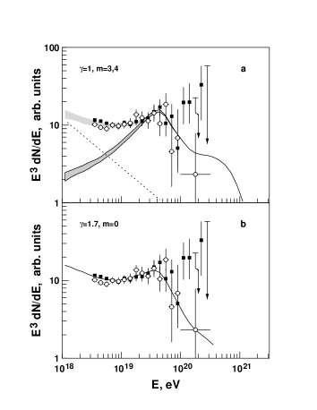
Figure 1: a) A fit of UHECR spectrum with flat extragalactic injection spectrum. Upper edge of shaded area is for $m$=4, lower - $m$=3. Galactic contribution is (dotted line) with $\gamma$=2.6. b) Fitting with steep injection spectrum ($\gamma$=1.7).

A different type of fit is illustrated in the bottom panel of Fig. 1. Extragalactic cosmic rays with injection spectrum E^-2.7 prevail down to 10¹⁸ eV. These cosmic rays are expected to be protons and He nuclei. Generally injection spectra steeper than E^-2.5 can fit the observed spectra without strong redshift evolution. The second knee is the result of $dE/dx$ due to pair production BGG ; BerGri . The galactic cosmic ray spectrum extends to about 10¹⁸ eV. The spectral shape of the extragalactic cosmic rays has to be flatter below 10¹⁸ eV to avoid overproducing lower energy cosmic rays. One possible explanation is the limited horizon of lower energy extragalactic cosmic rays because of scattering in extragalactic magnetic fields L04 .

Figure 2: Neutrino production in three simplified models for the source spectrum and evolution of UHECR. To enhance the contrast between different models, the source luminosity is extended out to $1+z_{max}=10$.

Cosmogenic (GZK) neutrino production. As shown in Fig. 1, different UHE cosmic ray source models, with different luminosities at $10^{19}$ eV, produce spectra consistent with observations. The differences at lower energy may be disguised by contributions from the galaxy, or by propagation effects. The model degeneracy can be broken by considering the neutrino flux produced by the UHECR via their interactions on the cosmic micro-wave background BZ69 ; S73 , the so-called GZK neutrino flux.

To make the point, we consider a set of simple power law models in a matter dominated cosmology, with a homogeneous distribution of UHECR sources. On cosmological time scales, the UHECR interact quickly with the CMB, so we model the production of GZK neutrinos as instantaneous with particle injection. We use the neutrino yields of Ref. ESS . The neutrino flux at Earth due to GZK production is

$$E_{\nu}\frac{d\Phi}{dE_{\nu}}(E_{\nu})=\int dtd\epsilon_{p}\frac{d\Gamma}{d\epsilon_{p}}E_{\nu}\frac{dy}{dE_{\nu}}(E_{\nu},\epsilon_{p},t)$$ (1)

where $\Gamma$ is the injection rate of UHECR and $y$ is the neutrino yield per proton injected with energy $\epsilon_{p}$, and $E_{\nu}$ is the neutrino energy today.

Equation 1 can be put into a more convenient form by defining $q=1+z$ and integrating over redshift. For a matter dominated cosmology, $H_{0}dt=-q^{-3/2}d(\ln q)$, where $H_{0}$ is the present day Hubble parameter. As a function of red shift, we model the UHECR injection rate as

$$\frac{d\Gamma}{d\epsilon_{p}}=q^{m}\epsilon_{p}^{-(1+\gamma)}A$$ (2)

where $\gamma$ is the integral spectral index of the source, $m$ describes the evolution of the co-moving source density, and $A$ is chosen to normalize the emissivity of UHECR sources to their energy density in the present Universe. We use ${\cal L}_{CR}=4.5\times{\rm 10}^{44}$ erg/Mpc³/yr as estimated by Waxman W95 . The neutrino yield can also be scaled with redshift. Defining the present day yield as $\frac{dy_{0}}{dE_{\nu}}(E_{\nu},E_{p})$, the yield from a previous epoch is

$$E_{\nu}\frac{dy}{dE_{\nu}}(E_{\nu},\epsilon_{p},z)=E_{\nu}\frac{dy_{0}}{dE_{\nu}}(q^{2}E_{\nu},q\epsilon_{p})$$ (3)

The factors of $q$ are due to the redshift of neutrino energy from production to the current epoch, and to the lowering of the reaction threshold due to the increased CMB temperature in the early Universe. Let $Y_{0}$ be the integrated yield from injecting an $E_{p}^{-(1+\gamma)}$ spectrum today: $E_{\nu}\frac{dY_{0\gamma}}{dE_{\nu}}(E_{\nu})=\int dE_{p}E_{p}^{-(1+\gamma)}E_{\nu}\frac{dy_{0}}{dE_{\nu}}(E_{\nu},E_{p})$. Then the integral yield at any other redshift is given by

$$\int d\epsilon_{p}\epsilon_{p}^{-(1+\gamma)}E_{\nu}\frac{dy}{dE_{\nu}}(E_{\nu},\epsilon_{p},t)=q^{\gamma}E_{\nu}\frac{dY_{0\gamma}}{dE_{\nu}}(q^{2}E_{\nu})$$ (4)

With these definitions, the GZK production integral can be expressed as an integral over redshift,

$$E_{\nu}\frac{d\Phi}{dE_{\nu}}(E_{\nu})=\frac{A}{H_{0}}\int_{0}^{q_{max}}d(\ln q)q^{(m+\gamma-\frac{3}{2})}E_{\nu}\frac{dY_{0\gamma}}{dE_{\nu}}(q^{2}E_{\nu})$$ (5)

Written as an integral over $\ln q$, it is straightforward to see which epoch dominates the neutrino flux. If $m+\gamma=1.5$ then all redshift intervals contribute with comparable importance. This is illustrated by the top panel of Fig. 2, where $m=0.5,\gamma=1$. The thin lines represent the contribution to the neutrino flux from epochs spaced equally in $\ln q$, and of equal width in $d(\ln q)$. The peak contribution for each interval occurs at an energy $E_{pk}(q)$, which scales with redshift as $E_{pk}(q)=E_{pk}(0)/q^{2}$. The sum of the thin lines, back to a red shift of $1+z_{max}=10$, gives the dotted curve - the predicted GZK neutrino flux for the model. The integrated flux is flat, with a width in $E_{\nu}$ of order $(1+z_{max})^{2}$.

Similarly, the middle panel illustrates a second model with equal contribution per epoch, although here there is no evolution ($m=0$) and the spectrum is correspondingly steeper ($\gamma=1.5$). The total cosmogenic neutrino flux is slightly lower because of the smaller number of interacting protons. The larger value of $\gamma$ is only evident through the different slope of the high energy part of the neutrino spectrum. In contrast, if $m+\gamma>1.5$ the neutrino flux is dominated by past epochs, as illustrated in the bottom panel of Fig. 2. This corresponds to the situation for a flat source model with significant evolution, $m=3,\gamma=1$. Note that this illustrative model is not realistic as the $(1+z)^{3}$ evolution continues to 1+$z_{max}$ = 10.

Figure 3: Neutrino production for the UHECR models shown in Fig. 1. The injection spectrum is cutoff at $E_{c}=3\times 10^{21}$ GeV and the source evolution breaks at $z_{max}=3$. Model results depend mildly on the cosmological model, $\Omega_{\Lambda}=0.0~{}{\rm or}~{}0.7$.

Discussion. The scaling analysis illustrates the combined importance of the UHECR spectrum and cosmological evolution in estimating the neutrino flux due to GZK production. For more realistic models, it is appropriate to consider other effects, such as a cosmological constant, a cutoff to the cosmic ray injection spectrum, and a cutoff or break in scale to the source evolution model. These effects alter the details of GZK production, but do not change the overall picture. Accordingly, Fig. 3 shows an order of magnitude difference in the GZK production for the two extreme UHECR models discussed in Fig. 1. Apart from the lower value of $z_{max}$, the steep source model with no evolution ($\gamma=1.7,m=0$) is similar to the middle panel of Fig. 2. The model with flat spectrum and cosmological evolution ($\gamma=1,m=3$) predicts an order of magnitude larger flux.

This brings us to the main point of this paper. The AUGER observatory, under construction, will measure the intensity and spectrum of UHECR. Above the GZK cutoff these are observations of the current Universe. Below the GZK cutoff it may be difficult to separate the old intergalactic cosmic rays from a population of young cosmic rays which originate within our own galaxy. Complementary to AUGER, experiments are being designed and constructed (ANITA, IceCube, Mediterranean km³, RICE), which may confirm the existence of GZK neutrinos. A next generation of experiments (EUSO, OWL, SalSA, X-RICE) is being planned which would provide sufficient statistics (10-100 GZK events per yr) to complement and expand the AUGER observations. Successful completion of one such experiment would be an important step toward understanding the sources of the highest energy particles in the Universe.

It is often argued that neutrino astronomy has value in that neutrinos allow observation of the interior of objects, whereas photons only allow observation of the surface. Solar neutrinos are an example, confirming theoretical models of the thermonuclear furnace in the sun, by direct observation of the core. The current discussion is similar. The “surface” is the interaction distance for super-GZK UHECR. The “interior” is the early Universe, where the evolution of UHECR sources can be directly observed through the GZK neutrino flux.

Acknowledgments. This research is supported in part by NASA Grant NAG5-10919. TS is also supported by the US Department of Energy contract DE-FG02 91ER 40626.

References

- (1) G. Cocconi, Nuovo Cimento, 3, 1433 (1956).
- (2) D.P. Torres & L.A. Anchordoqui, Rep. Prog. Phys., 67, 1663-1730 (2004).
- (3) P. Bhattacharjee & G. Sigl, Phys.Rept. 327, 109, (2000).
- (4) R.J. Protheroe & P.L. Biermann,
- (5) M. Takeda et al.(AGASA Collaboration), Phys.Rev.Lett. 81:1163, (1998);, see also the AGASA web page http://www-akeno.icrr.u-tokyo.ac.jp/AGASA.
- (6) R.U. Abbasi et al. (HiRes Collaboration) Phys.Rev.Lett. 92:151101 (2004).
- (7) K. Greisen, Phys. Rev. Lett. 16, 748 (1966); G.T. Zatsepin & V.A. Kuzmin, JETP Lett. 4, 78 (1966).
- (8) E. Waxman & J.N. Bahcall, Phys. Lett. B 226, 1 (2003)
- (9) T. Wibig & A.W. Wolfendale, astro-ph/0410624
- (10) R.U. Abbasi et al., (HiRes Collaboration), astro-ph/0407622.
- (11) V.S. Berezinsky, A.Z. Gazizov & S.I. Grigorieva, astro-ph/0204357; astro-ph/0210095
- (12) V.S. Berezinsky & S.I. Grigoreva, Astron. Astrophys., 199, 1 (1988).
- (13) M. Lemoine, astro-ph/0411173
- (14) V.S. Berezinsky & G.T. Zatsepin, Phys. Lett. 28b, 423 (1969); Sov. J. Nucl. Phys. 11, 111 (1970).
- (15) F.W. Stecker, Astroph. Space Sci. 20, 47 (1973).
- (16) R. Engel, D. Seckel & T. Stanev, Phys. Rev. D64:093010 (2001)
- (17) E. Waxman, Ap. J. 452, L1 (1995)