Dark Energy Constraints from the CTIO Lensing Survey

Abstract

We perform a cosmological parameter analysis of the 75 square degree CTIO lensing survey in conjunction with CMB and Type Ia supernovae data. For $\Lambda$CDM cosmologies, we find that the amplitude of the power spectrum at low redshift is given by $\sigma_{8}=0.81^{+0.15}_{-0.10}\ (95\%\ {\rm c.l.})$, where the error bar includes both statistical and systematic errors. The total of all systematic errors is smaller than the statistical errors, but they do make up a significant fraction of the error budget. We find that weak lensing improves the constraints on dark energy as well. The (constant) dark energy equation of state parameter, $w$, is measured to be $-0.89^{+0.16}_{-0.21}\ (95\%\ {\rm c.l.})$. Marginalizing over a constant $w$ slightly changes the estimate of $\sigma_{8}$ to $0.79^{+0.17}_{-0.14}\ (95\%\ {\rm c.l.})$. We also investigate variable $w$ cosmologies, but find that the constraints weaken considerably; the next generation surveys are needed to obtain meaningful constraints on the possible time evolution of dark energy.

1. Introduction

Observations of weak gravitational lensing, the coherent distortion in the images of distant galaxies, have advanced rapidly in the past four years. The first detections of weak lensing in blank fields were reported only a few years ago (Wittman et al., 2000; Kaiser et al., 2000; Van Waerbeke et al., 2000; Bacon et al., 2000; Rhodes, Refregier, & Groth, 2000). More recent lensing measurements (Hoekstra et al., 2002; Refregier et al., 2002; Bacon et al., 2003; Brown et al., 2003; Hamana et al., 2003; Jarvis et al., 2003; Van Waerbeke et al., 2005; Heymans et al., 2005) have used larger and/or deeper surveys to reduce the statistical errors, which scale as $N^{-1/2}$ where $N$ is the number of galaxies measured. Better techniques for reducing systematic errors have also been developed, resulting in interesting cosmological constraints from lensing surveys.

Shear correlations measured by lensing surveys determine the projected power spectrum of matter fluctuations in the Universe. These fluctuations are believed to have grown due to gravitational instability from the early universe to the present. The growth of fluctations from last scattering, $z=1100$, to the present is sensitive to the densities of dark energy and matter via the Hubble expansion rate. Further, the measured lensing signal depends on angular diameter distances to the source galaxies. Thus weak lensing observables probe the dark energy density through both the growth function and the geometric distance factors. Present lensing measurements are sensitive to redshifts $0\lesssim z\lesssim 1$.

As the size of weak lensing surveys increases and the statistical errors keep going down, it becomes more important to similarly reduce the systematic errors. There are a few different systematic errors which can contaminate a weak lensing signal at the level of typical cosmic shear measurements. The largest of these has typically been the corrections of the anisotropic point-spread-function (PSF). We have recently developed a principal component analysis approach to interpolating the PSF between the stars in the image using information from multiple exposures (Jarvis & Jain, 2005). The PSF pattern is found to be a function of only a few underlying variables. Therefore, we are able to improve the fits of this pattern by using stars from many exposures. We have applied it to the CTIO survey data presented in Jarvis et al. (2003) and have shown that the level of systematic error is well below the statistical errors. Indeed the measured $B$-mode in shear correlations is consistent with zero on all scales measured. In this paper we present a new parameter analysis of the CTIO lensing survey. With the reduced systematic error, we are able to extract information from the measured signal over nearly two decades in length scale.

Type Ia supernovae observations led to the discovery of the accelerated expansion of the universe (Riess et al.1998; Perlmutter et al.1999). By combining information from the CMB at $z=1100$, large-scale structure and SNIa, interesting constraints on dark energy have been obtained (Spergel et al., 2003; Bridle et al., 2003; Weller & Lewis, 2003; Alam et al., 2004; Saini et al., 2004; Tegmark et al., 2004; Wang & Tegmark, 2004; Seljak et al., 2005; Simon, Verde, & Jimenez, 2005; Rapetti et al., 2005; Jassal et al., 2005). Whether the dark energy density is constant or evolving with cosmic time is one of the most interesting observational questions. It is often expressed using the parameterization

$$w(a)=w_{0}+w_{a}(1-a),$$ (1)

where $w$ is the dark energy equation of state parameter $w=p/\rho$ and $a=1/(1+z)$ is the expansion scale factor (Chevallier & Polarski, 2001; Linder, 2003). The cosmological constant corresponds to $w_{0}=-1,w_{a}=0$. A non-zero value of $w_{a}$ corresponds to a time-dependent equation of state. We investigate three priors for $w$: $\Lambda$CDM ($w_{0}=-1,w_{a}=0$), constant $w$ ($w_{a}=0$) with $-3<w<0$, and variable $w$ with $-8<w<8$ and $-8<w_{a}<8$.

In §2 we briefly review our CTIO survey data and shape measurement technique, largely deferring to our previous papers (Jarvis et al., 2003; Jarvis & Jain, 2005) for more details. In §3, we present the results from the new reduction. We use these results to constrain cosmological parameters in §4, and conclude in §5.

2. Data

Our CTIO survey data was originally described in detail in Jarvis et al. (2003), and we refer the reader to that paper for most of the details about the data and the analysis. Here, we present a brief summary of the data set, and point out two significant changes in the analysis: our PSF interpolation and the dilution correction.

The data were taken at Cerro Tololo Interamerican Observatory (CTIO) in Chile from December, 1996 to July, 2000. We observed 12 fields, well separated on the sky, in low extinction but otherwise random locations. Each field is approximately 2.5 degrees on a side, giving us a total of 75 square degrees. The 50% completeness level occurs near $R=23.5$ for each field, although it varies somewhat between the fields. We impose limits of $19<R<23$, which gives about 2 million galaxies to use for our lensing statistics.

The shape measurements of the galaxies follow the techniques of Bernstein & Jarvis (2002). The galaxy shapes are measured using an elliptical Gaussian weight function which is matched to have the same ellipticity as the galaxy. (That is, we use a circular Gaussian in the sheared coordinate system in which the galaxy is round.) The observed ellipticity is then calculated as:

$$\mbox{\bf e}=e_{1}+ie_{2}=\frac{\int I(x,y)W(x,y)(x+iy)^{2}dxdy}{\int I(x,y)W(x,y)(x^{2}+y^{2})dxdy}$$ (2)

where $I$ is the intensity, $W$ is our Gaussian weight, $x$ and $y$ are measured from the (weighted) centroid of the image, and the boldface indicates that e is a complex quantity.

We correct for the effects of the point spread function (PSF) in two steps. First, we correct for the effect of the shape of the PSF by reconvolving the observed images with a spatially varying convolution kernel which is designed to make the stars round. The galaxies in the convolved images are thus no longer affected by the shape of the point spread function (PSF), but are still affected by the size of the PSF.

Since the convolution kernel is only measured where we have an observed star, and the PSF is far from uniform across each image, we need to interpolate between the stars. In our previous analysis, we used a separate interpolation for every image. For this analysis, however, we use our new principal component algorithm which uses the information from all of the images at once. This new method, which gives a better fit, is described in Jarvis & Jain (2005).

The effect of the size of the PSF is called dilution. A perfectly round PSF blurs the images of galaxies, which reduces the observed ellipticity. For a purely Gaussian PSF and Gaussian galaxies, the measured ellipticities are reduced by a factor $R$:

$$R=1-\frac{\sigma^{2}_{\rm psf}}{\sigma^{2}_{\rm gal}}$$ (3)

However, galaxies are certainly not Gaussian, and stars are only approximately Gaussian. In our previous analysis we used a formula intended to account fot the first order corrections due to the kurtosis of the galaxies and the PSF. Unfortunately, our formula was incorrect with respect to the PSF kurtosis, as pointed out by Hirata & Seljak (2003). They give a more accurate correction scheme which accounts for both kurtoses correctly to first order – we implement this scheme in the analysis presented below. Their formula is quite complicated to write, but is easy to implement, so we defer to their Appendix B for the relevant equations.

Finally, we estimate the shear, $\gamma$, from an ensemble of ellipticities using the formula:

$$\hat{\mbox{\boldmath$\gamma$}}=\frac{1}{2\mbox{$\cal R$}}\frac{\sum w_{i}\,\mbox{\bf e}_{i}}{\sum w_{i}}$$ (4)

where the responsivity, $\cal R$, describes how our mean ellipticity changes in the presence of an applied distortion. It generalizes the formula given in equation 3 to non-Gaussian shapes. The factor of 2 in the denominator above converts the ellipticity to shear, and $w$ is our weight function. We use the “easy” weight function given in Bernstein & Jarvis (2002) (Equation 5.36):

$$w=[e^{2}+(1.5\sigma_{\eta})^{2}]^{-1/2}$$ (5)

where $\sigma_{\eta}$ is the shape uncertainty in the sheared coordinates where the galaxy is circular. The corresponding responsivity, $\cal R$, is also given in Bernstein & Jarvis (2002) (Equation 5.33).

3. Weak Lensing Statistics

To describe the two-point statistics of our shear field, we use the aperture mass statistic (Schneider et al., 1998; Crittenden et al., 2002; Schneider et al., 2002; Pen et al., 2002).

The predictions from theory come in the form of the convergence power spectrum:

$$P_{\kappa}(\ell)=\frac{9}{4}\Omega_{0}^{2}\int_{0}^{\chi_{H}}d\chi\frac{g^{2}(\chi)}{a^{2}(\chi)}P_{3D}\left(\frac{\ell}{r(\chi)};\chi\right)$$ (6)

where $\chi$ is the radial comoving distance, $\chi_{H}$ is the horizon distance, $r(\chi)$ is the comoving angular distance, $a$ is the scale size of the universe, $P_{3D}$ is the three-dimensional power spectrum of the matter fluctuations, and

$$g(\chi)=\int_{\chi}^{\chi_{H}}d\chi^{\prime}p(\chi^{\prime})\frac{r(\chi^{\prime}-\chi)}{r(\chi^{\prime})}$$ (7)

where $p$ is the normalized (to give unit integral over $\chi$) redshift distribution of source galaxies. These predictions are not reliable for high values of $k$ ($k>10h{\rm Mpc}^{-1}$) (Smith et al., 2003) due to difficulties in predicting the non-linear growth.

The observed second moments are completely described using the two-point correlation functions:

$$\xi_{+}(\theta) = \langle\gamma({\bf r})\gamma^{*}({\bf r+\mbox{\boldmath$\theta$}})\rangle$$

$$\xi_{-}(\theta)+i\xi_{\times}(\theta) = \langle\gamma({\bf r})\gamma({\bf r+\mbox{\boldmath$\theta$}})e^{-4i\alpha}\rangle$$ (8)

where $\mbox{\boldmath$\theta$}=\theta e^{i\alpha}$ is the separation between pairs of galaxies, and treating the positions on the sky as complex values. The correlation functions are not measured at all on scales larger than the size of the survey fields (for this survey, at $\theta>200\arcmin$), which correspond to low $k$ values.

Using the information from the correlation function to obtain the power spectrum, or vice versa, requires an extrapolation away from the $k$ values which are well measured or well predicted. The aperture mass statistic is in some sense a compromise between these two statistics, since it can be calculated from either the power spectrum or the correlation function using only the range of $k$ values which are either predicted or measured, respectively:

$$\langle M_{\rm ap}^{2}\rangle(R) = \frac{1}{2\pi}\int\ell d\ell P_{\kappa}(\ell)W(\ell R)^{2}$$ (9)

$$= \frac{1}{2}\int\frac{\theta\,d\theta}{R^{2}}\left[\xi_{+}(\theta)T_{+}\left(\frac{\theta}{R}\right)+\xi_{-}(\theta)T_{-}\left(\frac{\theta}{R}\right)\right]$$

where we use the form suggested by Crittenden et al. (2002) for which we have:

$$W(\eta) = \frac{\eta^{4}}{4}e^{-\eta^{2}}$$

$$T_{+}(x) = \frac{x^{4}-16x^{2}+32}{128}e^{-x^{2}/4}$$

$$T_{-}(x) = \frac{x^{4}}{128}e^{-x^{2}/4}$$ (10)

The aperture mass therefore has both good predictions from theory and accurate measurements from the data.

While the integral in Equation 9 is technically from 0 to infinity, the $T$ functions drop off very quickly, so that the effective upper limit is really around $5R$. Our fields are $200\arcmin$ along the long diagonal, so we can measure the aperture mass up to $R=40\arcmin$. The lower limit, due to difficulties of measuring the correlation function on very small scales, is about $R=1\arcmin$.

The function $W(\ell R)$ is a narrow function around $\ell R=\sqrt{2}$, so this corresponds to a range in $\ell$ of approximately $120<\ell<5000$.

The other big advantage to the aperture mass statistic is that it provides a natural check for systematics. Weak lensing should only produce a curl-free $E$-mode component, so any $B$-mode observed in the shear field represents a systematic error of some sort. The aperture mass statistic has a $B$-mode counterpart which can be likewise calculated from the correlation functions as:

$$\langle M_{\times}^{2}\rangle(R)=\frac{1}{2}\int\frac{\theta\,d\theta}{R^{2}}\left[\xi_{+}(\theta)T_{+}\left(\frac{\theta}{R}\right)-\xi_{-}(\theta)T_{-}\left(\frac{\theta}{R}\right)\right]$$ (11)

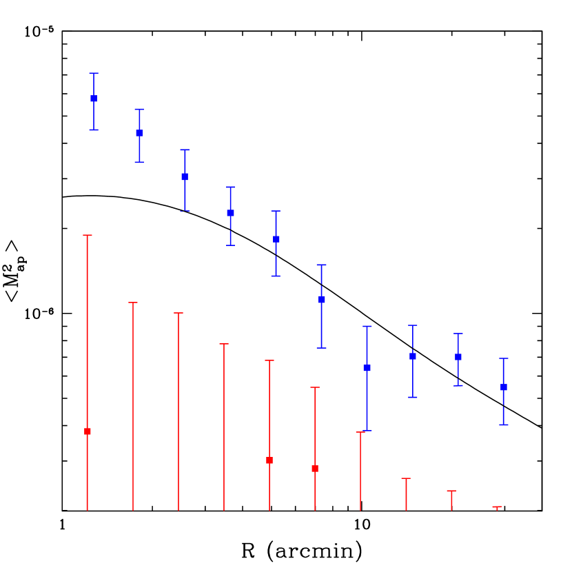
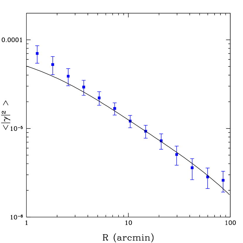
Figure 1.— The aperture mass (left) and shear variance (right) measurements for our CTIO survey data. For the left plot, the blue (upper) points are the $E$-mode measurements, $\langle M_{\rm ap}^{2}\rangle(R)$ and the red (lower) points are the $B$-mode contamination, $\langle M_{\times}^{2}\rangle(R)$. For the right plot, the blue points are the total shear variance, including any potential $B$-mode contamination. In both cases, the black curve is the best fit flat $\Lambda$CDM model found in §4.

Figure 1 shows the results for our reanalysis. The blue points are the $E$-mode signal, and the red points are the $B$-mode contamination. Points separated by at least one other point are very nearly uncorrelated. The black curve is the best fit flat $\Lambda$CDM model found below.

The $B$-mode is seen to be consistent with zero at all scales, which was not the case for our previous analysis. Further, in Jarvis & Jain (2004) we show that the measured ellipticity correlation function of stars, which is another measure of systematic errors, is one to two orders of magnitude smaller than the expected lensing signal at all scales. Therefore, we can now confidently use all of the aperture mass values from $1\arcmin$ to $40\arcmin$ for our constraints on cosmology.

In addition to the aperture mass, we also measure the variance of the mean shear in circular apertures:

$$\langle|\gamma|\rangle^{2}(R) = \frac{1}{2\pi}\int\ell d\ell P_{\kappa}(\ell)\frac{4J_{1}(\ell R)^{2}}{(\ell R)^{2}}$$ (12)

$$= \int_{0}^{2R}\frac{\theta\,d\theta}{R^{2}}\xi_{+}(\theta)S_{+}\left(\frac{\theta}{R}\right)$$

where

$$S_{+}(x)=\frac{1}{\pi}\left(4\arccos(x/2)-x\sqrt{4-x^{2}}\right)$$ (13)

Figure 1 shows the results for the shear variance statistic. There is no $E/B$ decomposition for this statistic. We assume implicitly that there is no $B$-mode contamination in the shear variance measurements, which seems reasonable given the low $B$-mode seen for the aperture mass.

The usefulness of this statistic is that it is able to probe the power spectrum at somewhat smaller $\ell$ values than the aperture mass statistic. The upper limit in the integral in Equation 12 is only $2R$, so we can calculate the shear variance up to $R=100\arcmin$ with our data. This probes the power spectrum down to $\ell$ of about 70. This leads to a total dynamic range for both statistics of almost 2 orders of magnitude. The shear variance below $R=50\arcmin$ is degenerate with the aperture mass, so for our constraints, we only use the shear variance at large values of $R$ where it is providing extra information.

In Figure 1, we also show the overall best fit $\Lambda$CDM model (see §4). This fit has a $\chi^{2}$ of 7.7, for effectively 6 degrees of freedom, yielding a reduced $\chi^{2}$ of 1.28.

4. Analysis

4.1. Dark Energy Constraints from Weak Lensing

Our lensing measurement constrains the shear power spectrum, which is a weighted projection of the mass power spectrum. The constraints on dark energy arise from two sources. The first is the angular diameter distances to the lens, to the source, and between the lens and the source that enter into the projection. The second is the amplitude of the power spectrum. The dark energy component alters the expansion rate of the universe at redshifts below about 2 (at least if its evolution is not too different from a cosmological constant). This in turns affects the growth of structure. Since the CMB fixes the amplitude of the power spectrum at $z=1100$, the lensing measurement of the amplitude at low redshift measures the growth function. See Hu & Jain (2004) for a detailed discussion.

We assume that massive neutrinos make a negligible contribution to the matter density, that the primordial power spectrum index has no running and that the universe is spatially flat. The shape of the mass power spectrum is then specified by the baryon density $\mbox{$\Omega_{\rm b}$}h^{2}$, the matter density $\mbox{$\Omega_{\rm m}$}h^{2}$, and the primordial spectrum. Following the WMAP convention, we use the scalar amplitude $A_{\rm s}$ and spectral index $n$ such that the shape of the primordial power spectrum is $\mbox{$A_{\rm s}$}(k/k_{0})^{(n-1)}$, where $k_{0}=0.05$ Mpc^-1 is the normalization scale. The current uncertainties in these parameters are at the 10% level or better. Thus the power spectrum as a function of $k$ in Mpc^-1 (not $h$ Mpc^-1) in the matter dominated regime can be considered as largely known.

The amplitude of the power spectrum at a given redshift depends on the initial normalization $A_{\rm s}$ and the “growth function” $G$ defined by

$$P(k,z)=\left[\frac{1}{1+z}\frac{G(z)}{G_{0}}\right]^{2}P(k,0)\,,$$ (14)

where $G_{0}\equiv G(z=0)$ and we assume that all relevant scales are sufficiently below the maximal sound horizon of the dark energy.

The normalization of the linear power spectrum today is conventionally given at a scale of $r=8h^{-1}$Mpc and can be approximated as (Hu & Jain, 2004)

$$\sigma_{8}~{}\approx~{}\frac{\mbox{$A_{\rm s}$}^{1/2}}{0.97}\left(\frac{\mbox{$\Omega_{\rm b}$}h^{2}}{0.024}\right)^{-0.33}\left(\frac{\mbox{$\Omega_{\rm m}$}h^{2}}{0.14}\right)^{0.563}~{}\times(3.123h)^{(n-1)/2}\left(\frac{h}{0.72}\right)^{0.693}\frac{G_{0}}{0.76}\,,$$ (15)

Thus a measurement of $\sigma_{8}$, in conjunction with constraints on the other parameters in the above equation from the CMB, constrains a combination of dark energy parameters that affect $G_{0}$. Note that while the equation above illustrates how the dark energy parameters are linked to others, we do not actually use it in our parameter analysis. Instead we use the projection integral of Equation 6 which includes the full range of redshifts probed by our survey. The peak contribution to the lensing correlations is from $z\simeq 0.3$, though the maximum sensitivity to $w$ is at $z\simeq 0.4$ as discussed below. Combining our measurement with others such as Type Ia supernovae, which are sensitive to different redshifts, enables a probe of the time dependence of dark energy parameters. With photometric redshifts, this could be done with the lensing data alone using the auto and cross-spectra in redshift bins.

The dark energy modifies the expansion of the universe according to the equation (for a flat universe)(e.g. Linder & Jenkins, 2003):

$$H^{2}(a)=H_{0}^{2}\left[\mbox{$\Omega_{\rm m}$}a^{-3}+\mbox{$\Omega_{\rm de}$}e^{-3\int_{1}^{a}{\frac{da}{a}(1+w(a))}}\right]$$ (16)

where the dark energy density is $\mbox{$\Omega_{\rm de}$}(a)=8\pi G\rho_{\rm de}/3H(a)^{2}$, its equation of state is $w(a)=p_{\rm de}/\rho_{\rm de}$, and we indicate the present time values, $\mbox{$\Omega_{\rm m}$}(a=1)$ and $\mbox{$\Omega_{\rm de}$}(a=1)$ as simply $\Omega_{\rm m}$and $\Omega_{\rm de}$.

Distances are then given by

$$\chi(a)=\int_{a}^{1}{\frac{da^{\prime}c}{H(a^{\prime}){a^{\prime}}^{2}}}$$ (17)

and the growth function $G$ depends only on the dark energy throught the equation:

$$\frac{d^{2}G}{d\ln a^{2}}+\left[\frac{5}{2}-\frac{3}{2}w(a)\mbox{$\Omega_{\rm de}$}(a)\right]\frac{dG}{d\ln a}+\frac{3}{2}[1-w(a)]\mbox{$\Omega_{\rm de}$}(a)G=0\,.$$ (18)

When we use a constant $w$ parameterization, it is equivalent to a measurement of $w$ at the redshift for which the errors in the constant and time-dependent piece (in a Taylor expansion) are uncorrelated. See Hu & Jain (2004) for a discussion of this pivot redshift, which we find (§4.2.3) to be about $0.4$ for our survey (when combined with the CMB and SN priors as described below).

4.2. Joint Constraints

We use the results from WMAP (Spergel et al., 2003) as priors for our analysis. Specifically, we use the Monte Carlo Markov Chain (MCMC) calculated by Verde et al. (2003). We choose to use the less restrictive prior of $w>-3$ rather than $w>-1$ in order to be as conservative as possible. However, we do have a hard prior that $\mbox{$\Omega_{\rm k}$}=0$. While WMAP has constrained this to be $0.02\pm 0.02$ for pure $\Lambda$CDM, and there is theoretical bias in believing it is exactly 0, it is worth emphasising that our dark energy constraints would be weakened if this prior were relaxed.

Each step in the Markov chain contains a value for each of the following parameters: $\omega_{\rm b}=\mbox{$\Omega_{\rm b}$}h^{2}$ is the density of baryons; $\omega_{\rm c}=\mbox{$\Omega_{\rm c}$}h^{2}$ is the density of cold dark matter; $\theta_{\rm A}$ is the angular scale of the acoustic peaks; $n$ is the spectral slope of the scalar primordial density power spectrum; $Z=\exp(-2\tau)$ is related to the optical depth ($\tau$) of the last scattering surface; $A_{\rm s}$ is the overal amplitude of the scalar primordial power spectrum; $h=H_{0}/100$ is the Hubble constant; $w$ is the equation of state parameter for the dark energy.

The parameters $\theta_{A}$ and $Z$ are not directly relevant to the aperture mass statistic which we have measured, so we marginalize over these two. The others define a cosmology from which we can predict the aperture mass statistic on the scales where we have measured it. We present results for selected parameters below, these are obtained by a full marginalization over all the other parameters listed above.

For the linear power spectrum, we use the transfer function of Bardeen et al. (1986). We then estimate the non-linear power spectrum using the halo-based model of model of Smith et al. (2003). Their fitting formulae provide a means of estimating the quasi-linear and non-linear halo contributions to the power spectrum based on the linear value and the effective spectral index. This model agrees with the results of $N$-body simulations better than the simpler formula of Peacock & Dodds (1996). The nonlinear correction affects the predicted variance in the mass aperture statistic on scales below about 4 arcminutes.

We also note that the model of Smith et al. (2003) that we use does not include $w$ directly. We correctly take it into account for the growth factor and the distances, but Mainini et al. (2003) and Klypin et al. (2003) show that dark energy changes the virial density contrast, $\Delta_{c}$, which results in changes in the power spectrum at high $k$ values ($k>1\ h{\rm Mpc}^{-1}$). However, the effect is smaller than the expected error in the non-linear model even for a $w\simeq-0.5$ cosmology.

From the predicted power spectrum, we calculate the aperture mass and shear variance statistics using Equations 6, 9, and 12. Our data then give a likelihood value for each cosmology, which we combine with the CMB likelihood from the MCMC.

We also use the recent supernova measurements of Riess et al. (2004) to further constrain the results. For this, we use the $\chi^{2}$ calculation program of Tonry et al. (2003).

4.2.1 $\Lambda$CDM Models

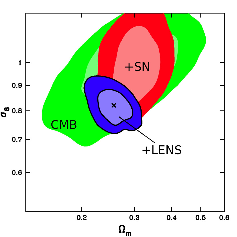
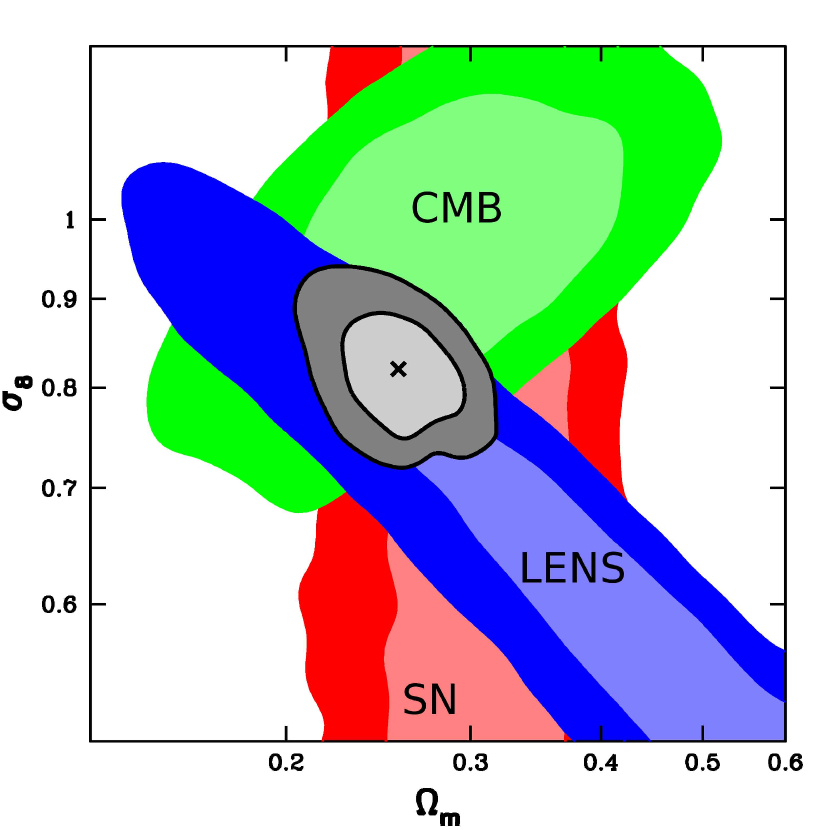
Figure 2.— Contour plots of $\chi^{2}$ for the $(\mbox{$\Omega_{\rm m}$},\sigma_{8})$ plane. The left plot shows the effect of adding the data sets sequentially, starting with the CMB constraints, then adding the supernova and lensing data. The right plot shows contours for each of the three data sets separately. In each case the contours enclose the 68% and 95% confidence regions. The $\times$ is the best fit model. All other parameters are marginalized over as discussed in the text.

With dark energy priors of $w=-1$ and $w_{a}=0$, the likelihood constraints are non-trivial contours through a five-dimensional parameter space. However, most of the gain in constraining power from the addition of the lensing data comes in the quantities $\Omega_{\rm m}$ and $\sigma_{8}$. We show the error contours projected onto the $\mbox{$\Omega_{\rm m}$}-\sigma_{8}$ plane in Figure 2. The left plot shows the contours starting with the CMB data set, and sequentially adding the supernova and lensing data. The right plot shows the contours in the $\mbox{$\Omega_{\rm m}$}-\sigma_{8}$ plane separately for each of the three data sets to indicate the degree of their complementarity, which is why their combination leads to the tight overall constraints. In both plots, the contours correspond to 68% and 95% confidence regions ($\Delta\chi^{2}$ = 2.30 and 6.17). The crosses are at the peak likelihood in the projected plane, which is at: ($\mbox{$\Omega_{\rm m}$}=0.26$, $\sigma_{8}=0.82$).

4.2.2 Constant $w$ Models

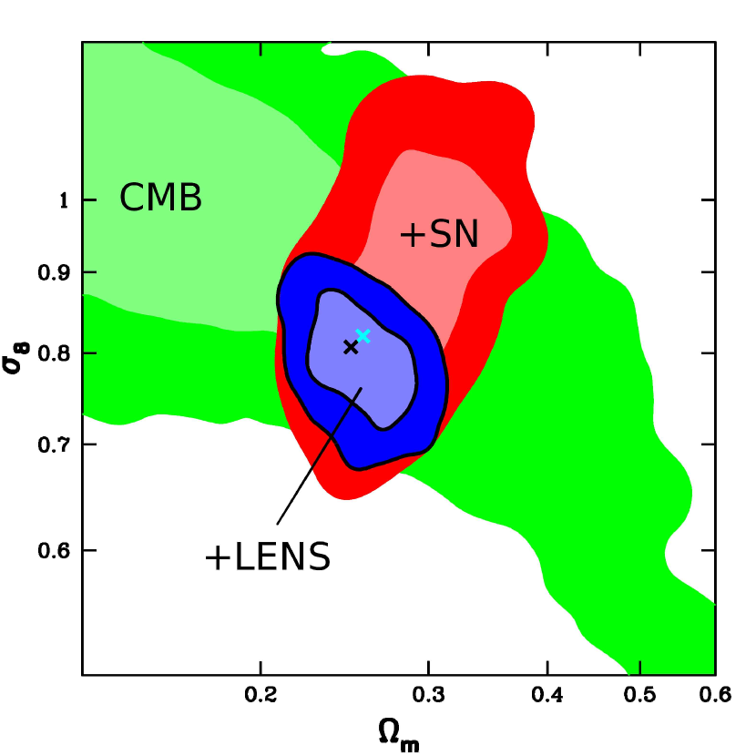
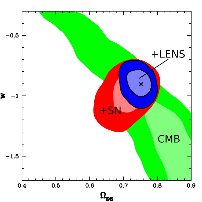
Figure 3.— Contour plots of $\chi^{2}$ for the $(\mbox{$\Omega_{\rm m}$},\sigma_{8})$ plane (left) and the $(\mbox{$\Omega_{\rm de}$},w)$ plane (right) for the constant $w$ dark energy models. Both plots show the effect of adding the data sets sequentially. In each case the contours enclose the 68% and 95% confidence regions. The black $\times$’s are the best fit models in each plane. The cyan $\times$ in the left plot is the best fit from the $\Lambda$CDM prior (Figure 2).

We show the uncertainty contours for the dark energy priors of $-3<w_{0}<0$ and $w_{a}=0$ in Figure 3. The left plot give the projection in the $\mbox{$\Omega_{\rm m}$}-\sigma_{8}$ plane, which indicates that allowing $w$ to be free does not significantly worsen the constraints on $\Omega_{\rm m}$ and $\sigma_{8}$ compared to the pure $\Lambda$CDM model. The $\mbox{$\Omega_{\rm de}$}-w$ plot (right) shows why. While none of the three data sets individually have tight constraints in this plane, the combination of all three leads to a fairly tight contour near (and consistent with) $w=-1$. The peak likelihood models in the two projections are: ($\mbox{$\Omega_{\rm m}$}=0.25$, $\sigma_{8}=0.79$) and ($\mbox{$\Omega_{\rm de}$}=0.75$, $w=-0.90$).

4.2.3 Variable $w$ Models

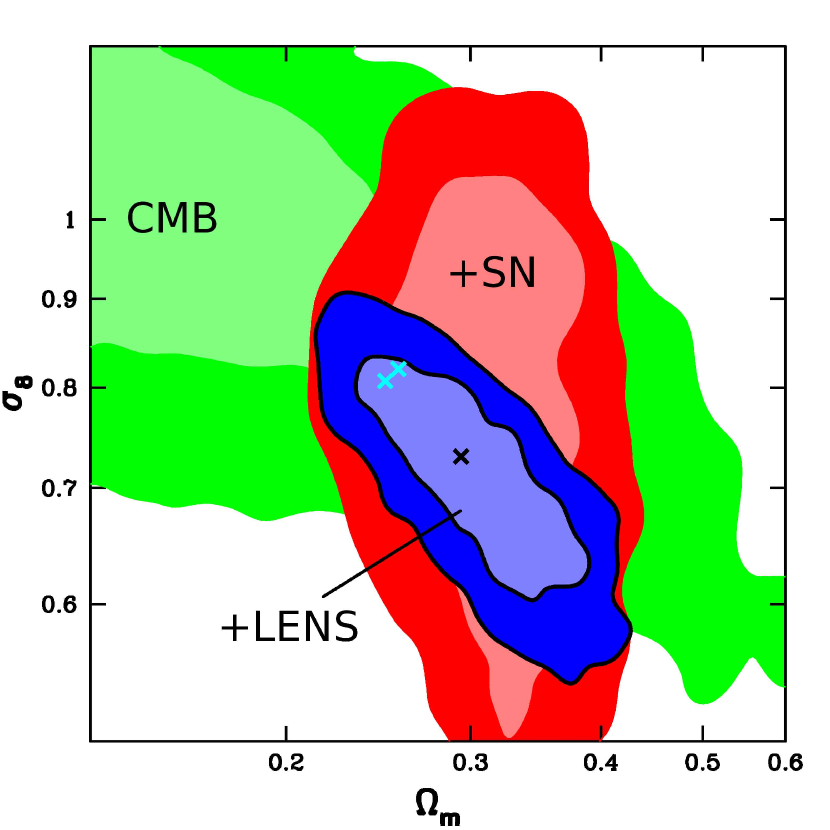
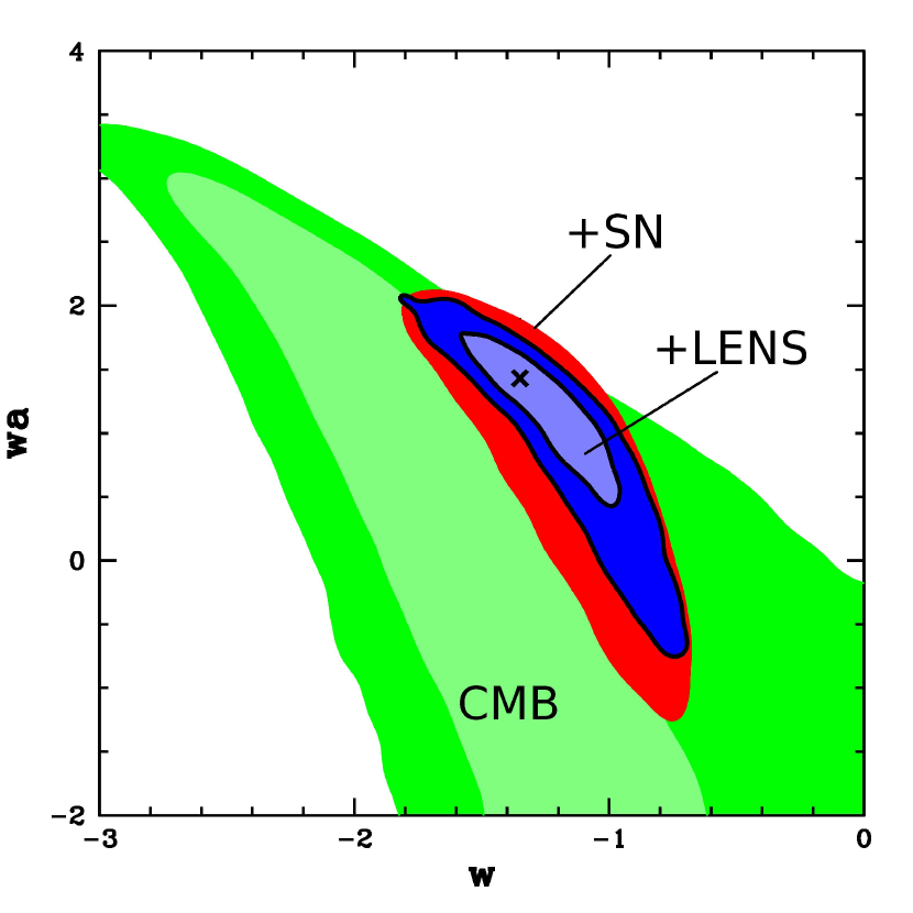
Figure 4.— Contour plots of $\chi^{2}$ for the $(\mbox{$\Omega_{\rm m}$},\sigma_{8})$ plane (left) and the $(w_{0},w_{a})$ plane (right) for the variable $w$ dark energy models. Both plots show the effect of adding the data sets sequentially. In each case the contours enclose the 68% and 95% confidence regions. The black $\times$’s are the best fit models in each plane. The cyan $\times$’s in the left plot are the best fits from the $\Lambda$CDM and constant $w$ priors (Figures 2 and 3).

Finally, we consider dark energy priors of $-8<w_{0}<8$ and $-8<w_{a}<8$. It turns out that some of the dark energy models in this range have $\Omega_{\rm DE}(z=1100)\approx 1$. That is, the mass-energy of the universe was essentially all dark energy at the epoch of recombination. This seems to be ruled out by WMAP data (Caldwell et al., 2003; Caldwell & Doran, 2004; Wang & Tegmark, 2004). Therefore, we make the additional prior that $\Omega_{\rm DE}(z=1100)<0.5$. In practice, all the models have $\Omega_{\rm DE}(z=1100)\approx 0$ or $1$, so this contraint is effectively $\Omega_{\rm DE}(z=1100)\approx 0$.

Given this constraint, the primary effect of dark energy on the CMB is through the distance to the last-scattering surface, $d_{\rm LSS}$. Therefore, we approximate the CMB likelihoods by using the WMap constant-$w$ Markov chain mentioned above, modifying the dark energy parameters to maintain a constant $d_{\rm LSS}$. Specifically, for each line in the Markov chain, we determine $d_{\rm LSS}$ from the values of $\Omega_{m}$ and $w$; we select $w_{a}$ from $-8<w_{a}<8$; then we determine what $w_{0}$ with this $w_{a}$ and the same $\Omega_{m}$ maintain the given value of $d_{\rm LSS}$, and we write these values out as a line in a new pseudo-chain.

The main approximation in this process is that we neglect the difference of the integrated Sachs-Wolfe (ISW) effect between the two models. There is some indication that for some of the models that fall within our contours (Figure 4, right), the ISW may spread the first peak in the power spectrum of the CMB enough to disfavor these models by 1 or 2 sigma. However, we defer a more detailed study of this effect to future work.

The error contours projected onto the $\mbox{$\Omega_{\rm m}$}-\sigma_{8}$ plane and the $w_{0}-w_{a}$ plane are shown in Figure 4. With this much freedom in the models, we do finally lose much of our constraining power. Even with all three data sets, the error contours are still quite large. The $\mbox{$\Omega_{\rm m}$}-\sigma_{8}$ plot (left) shows that allowing $w$ to vary with cosmological time does significantly worsen the constraints, allowing much lower values of $\sigma_{8}$.

Also, while lensing does significantly reduce the allowed parameter space in the $\mbox{$\Omega_{\rm m}$}-\sigma_{8}$ plane, this reduction has only a small effect in the $w_{0}-w_{a}$ plane, so that our constraints there are not much better than those for the CMB + SN data alone. The data are consistent with a cosmological constant ($w_{0}=-1,w_{a}=0$) at the 95% confidence level, but $w_{a}$ may range as high as 2.

We can use the direction of the contours in the $w_{0}-w_{a}$ plane to determine the redshift at which we have the strongest constraints on the dark energy. If we change variables from $\{w(z=0),w_{a}\}$ to $\{w(z=0.4),w_{a}\}$, the likelihood contour becomes roughly vertical. This indicates that our pivot redshift, or “sweet spot” (Huterer & Turner, 2001; Weller & Albrecht, 2002; Hu, 2002; Hu & Jain, 2004), where the constraints of the dark energy are strongest, is at a redshift of about $0.4$. (Of course, the banana shape makes this impossible to do precisely, so $z_{\rm piv}=0.4$ is just an approximate value.) We constrain $w$ at this redshift, marginalizing over $w_{a}$ (and everything else) below.

4.3. Systematic Errors

Systematic errors are harder to estimate than statistical errors, since by their nature they contaminate the data in unknown ways. There are four systematic errors which we investigate and attempt to estimate: residual anisotropic PSF as estimated by the residual $B$-mode, calibration error, redshift distribution error, and errors in the non-linear prediction. For shorthand, we refer to these as B, CAL, Z, and NL respectively.

When estimating the contributions of these systematic uncertainties to our error budget, we limit our consideration to constraints on single parameters, fully marginalized over all the other parameters. First we calculate the 95% error bars with only the statistical errors. Then, for each systematic effect, we change our handling of the effect as described more completely below for each case. When we do this, the 95% confidence intervals move around somewhat. We define the upper systematic error to be the maximum upper limit of the confidence interval allowed by the various changes minus the nominal upper limit with only the statistical errors. Likewise the lower systematic error is the lower limit with only the statistical errors minus the minimum allowed lower limit. Finally, we (conservatively) estimate the total error as the sum of the statistical errors and each of the systematic errors added linearly, not in quadrature.

For the residual PSF (B) systematic, we implement the same technique we used in Jarvis et al. (2003), namely running the analysis with the $B$-mode contamination added to and subtracted from the $E$-mode signal. Most types of contamination either add power (roughly) equally to the $E$ and $B$ modes, in which case the subtraction is appropriate, or mix power between the two modes while conserving total signal, in which case the addition is appropriate. We allow for both possibilities to estimate how the contamination could be affecting the cosmological fits.

The calibration (CAL) uncertainty includes errors in the dilution calculation, the responsivity formula, and possibly biases in the shape measurements. This systematic was the subject of significant discussion at the recent IAU symposium 225. There seem to be calibration differences of order 5% in shear estimators between different methods. Tests with simulated images with known shears indicate that we have calibration errors of less than 2% (Heymans et al., 2005), but we allow for $\pm$ 5% in our shear values as a conservative estimate of this systematic.

For the redshift calibration (Z) of our survey, there are two public redshift surveys with depths similar to our observations: the Caltech Faint Galaxy Redshift Survey (Cohen et al., 2000) (CRS), and the Canada-France Redshift Survey (Lilly et al., 1995) (CFRS). We argue in Jarvis et al. (2003) that the CRS is a better choice, since it is more complete in the $R$ filter band pass used for our observations. However, switching to the CFRS distribution allows us to estimate the uncertainties due to the redshift calibration. Also, since we only have one other survey to use, we cannot run symmetric plus and minus versions of this test. So when the 95% confidence limit moved inward for a value, we take the absolute value of the change as the measure of the systematic error, since a different redshift survey might have moved the limit a similar amount outward.

Finally, for the non-linear predictions (NL), we used the Smith et al. (2003) model, which were an improvement over that of Peacock & Dodds (1996). Switching back to the older model should give us a rough (over-)estimate of the remaining uncertainties due to the non-linear modelling. Again, we cannot run symmetric tests, so we take the absolute value of any change as a measure of the systematic error.

Since this technique is non-standard and may be confusing, an example with the actual values might help explain it. For the CAL test with the $\Lambda$CDM prior, when we multiplied the shear data by 1.05 (for the +5% test), the upper limit of the 95% confidence interval for $\sigma_{8}$ moved from 0.910 to 0.929, and increase of 0.019. This is our estimate of the positive systematic error. Similarly, in the -5% CAL test, the lower limit decreased, providing the negative systematic error for $\sigma_{8}$.

In Table 1, we present the statistical and systematic error estimates for $\Omega_{\rm m}$, $\sigma_{8}$, $w_{0}$ and $w_{a}$, for each of our dark energy priors. The first two columns present the estimates for each value with and without the lensing data, marginalized over all other parameters, and quoting only the statistical errors. The next four columns show the estimated systematic error due to each effect listed above. The final column includes the total uncertainty with the systematic errors added linearly with the statistical uncertainty. Note that we make no attempt to estimate the systematic errors present in the CMB or SN data.

Table 1Fully Marginalized Parameter Constraints (95% c.l.)

Parameter	CMB+SN	+Lensing	Estimated Systematic Errors				Final
	Constraint	(stat. only)	B	CAL	Z	NL	Estimate
$w_{0}=-1$, $w_{a}=0$ prior:
$\Omega_{\rm m}$	$0.301^{+0.07}_{-0.07}$	$0.256^{+0.05}_{-0.05}$	${}^{+0.005}_{-0.001}$	${}^{+0.008}_{-0.003}$	${}^{+0.008}_{-0.005}$	${}^{+0.000}_{-0.000}$	$0.256^{+0.07}_{-0.06}$
$\sigma_{8}$	$0.953^{+0.27}_{-0.18}$	$0.812^{+0.10}_{-0.09}$	${}^{+0.028}_{-0.006}$	${}^{+0.019}_{-0.006}$	${}^{+0.020}_{-0.007}$	${}^{+0.001}_{-0.001}$	$0.812^{+0.17}_{-0.11}$
$-3<w_{0}<0$, $w_{a}=0$ prior:
$\Omega_{\rm m}$	$0.285^{+0.08}_{-0.07}$	$0.254^{+0.05}_{-0.04}$	${}^{+0.005}_{-0.001}$	${}^{+0.006}_{-0.005}$	${}^{+0.006}_{-0.001}$	${}^{+0.000}_{-0.000}$	$0.254^{+0.07}_{-0.05}$
$\sigma_{8}$	$0.846^{+0.29}_{-0.17}$	$0.790^{+0.11}_{-0.10}$	${}^{+0.022}_{-0.015}$	${}^{+0.018}_{-0.012}$	${}^{+0.019}_{-0.012}$	${}^{+0.001}_{-0.001}$	$0.790^{+0.17}_{-0.14}$
$w$	$-0.935^{+0.16}_{-0.28}$	$-0.894^{+0.14}_{-0.16}$	${}^{+0.006}_{-0.016}$	${}^{+0.005}_{-0.017}$	${}^{+0.005}_{-0.019}$	${}^{+0.001}_{-0.000}$	$-0.894^{+0.16}_{-0.21}$
$-8<w_{0}<8$, $-8<w_{a}<8$, $\Omega_{\rm DE}(z=1100)<0.5$ prior:
$\Omega_{\rm m}$	+0$0.29^{+0.11}_{-0.06}$	+0$0.29^{+0.11}_{-0.07}$	${}^{+0.009}_{-0.000}$	${}^{+0.001}_{-0.000}$	${}^{+0.009}_{-0.001}$	${}^{+0.000}_{-0.000}$	+0$0.29^{+0.13}_{-0.07}$
$\sigma_{8}$	+0$0.79^{+0.32}_{-0.35}$	+0$0.74^{+0.13}_{-0.17}$	${}^{+0.044}_{-0.029}$	${}^{+0.013}_{-0.016}$	${}^{+0.024}_{-0.000}$	${}^{+0.000}_{-0.000}$	+0$0.74^{+0.21}_{-0.22}$
$w_{0}$	$-1.17^{+0.50}_{-0.57}$	$-1.14^{+0.41}_{-0.53}$	${}^{+0.008}_{-0.044}$	${}^{+0.006}_{-0.020}$	${}^{+0.016}_{-0.004}$	${}^{+0.002}_{-0.000}$	$-1.14^{+0.45}_{-0.60}$
$w_{a}$	+0$1.36^{+0.75}_{-1.79}$	+0$1.48^{+0.53}_{-1.57}$	${}^{+0.101}_{-0.258}$	${}^{+0.021}_{-0.055}$	${}^{+0.038}_{-0.124}$	${}^{+0.013}_{-0.082}$	+0$1.48^{+0.70}_{-2.09}$
$w(z=0.4)$	$-0.90^{+0.20}_{-0.33}$	$-0.87^{+0.13}_{-0.24}$	${}^{+0.005}_{-0.047}$	${}^{+0.000}_{-0.028}$	${}^{+0.002}_{-0.007}$	${}^{+0.000}_{-0.001}$	$-0.87^{+0.14}_{-0.32}$

It is apparent that the systematic uncertainties in our survey are smaller than the statistical uncertainties for each of the above cosmological parameters. However, there is still significant room for improvement in all of these sources of systematic errors. Future lensing surveys which expect to reduce the statistical uncertainties by a factor of order 10 will need to address these systematics so that they do not dominate the final error budget. And while the systematic errors due to the non-linear modelling are essentially completely negligible for our survey, they will be more significant for lensing surveys with smaller fields than ours.

5. Discussion

We have used our measurement of the shear two-point correlations to constrain the clustering of mass at redshifts $z\sim 0.3$ and the density and equation of state of dark energy. This has been done by combining the lensing information with the CMB and supernovae data. The three probes are sufficiently complementary that the joint contraints are significantly better than from any one or two methods.

We find that the primary sytematic effects on our lensing data are the redshift distribution of the galaxies, the overall calibration of the shear estimates, and the systematic error due to the coherent PSF anisotropy. With our new analysis, the total effect of these three systematics is smaller than the statistical errors. The PCA technique has substantially reduced the contribution of the $B$-mode, which used to be the dominant systematic error (Jarvis et al., 2003). We are continuing to work on methods to reduce this and the calibration uncertainty.

Improving the redshift distribution would require more data: either a larger redshift survey of similar depth as our data, or imaging the galaxies in three or four other filters to measure photometric redshifts. As discussed below, this second option would also allow us to bin the galaxies and make tomographic measurements.

We have necessarily made some choices of priors and datasets in our parameter analysis. The datasets we have used in addition to the lensing data are the WMAP first year extended data (Verde et al., 2003) (which also include CBI and ACBAR data) and the Riess et al. (2004) Type 1a Supernovae data. We have assumed that the universe is spatially flat; weakening this assumption significantly weakens constraints on dark energy, especially if $w$ is allowed to vary in time. We have also assumed no tensor contribution to the CMB power spectrum, that the primordial power spectrum is an exact power law (no running), and we have neglected the effects of massive neutrinos on the power spectrum. Current upper limits from cosmology (see e.g. Seljak et al., 2005) are below 1 electron volt for the the sum of neutrino masses. Allowing for massive neutrinos could lead to (at most) a few percent increase in our estimated $\sigma_{8}$, as the presence of massive neutrinos suppresses the power spectrum on scales that affect our observed shear correlations, but would not lead to interesting constraints on the neutrino mass.

Combining our data with CMB and SN data, our investigation of dark energy models show no evidence for the dark energy being different from a standard cosmological constant. Constant $w$ models are consistent with $w=-1$, and variable $w$ models are consistent with $w_{a}=0$. The constraints on dark energy from weak lensing come from a range of redshifts centered at $z\sim 0.3$, and extending by about $0.2$ in redshift on either side. Thus the measurements of its density and of $w$ should be interpreted with this redshift range in mind. When we combine our data with supernova data, we are using information from different redshifts, and the combined data have a pivot redshift of about $0.4$, where $w$ is best measured. At this redshift, we also find that $w$ is consistent with $-1$.

Our analysis can be compared with other recent work that combines CMB and supernova data with galaxy clustering, the abundance of galaxy clusters, the clustering of the Lyman alpha forest and other probes (Spergel et al., 2003; Weller & Lewis, 2003; Tegmark et al., 2004; Wang & Tegmark, 2004; Seljak et al., 2005; Rapetti et al., 2005). It is a powerful consistency check that these different methods appear to agree in their conclusions. It is interesting to compare the different redshift ranges probed by these methods, and explore constraints on the time dependence of the equation of state (e.g. Linder, 2003; Huterer & Cooray, 2005).

The prospects for constraining dark energy with future lensing surveys are very interesting. With a well designed survey and the recent analysis techniques, it can be hoped that systematic errors would stay at levels comparable to statistical errors. The addition of tomographic information with photometric redshifts would allow for significantly better constraints on cosmological parameters from lensing alone (Hu, 1999). The use of three point correlations would allow for some independent checks on systematics as well as improved constraints on cosmological parameters (see Pen et al. 2003; Jarvis, Bernstein & Jain 2004 for detections of the lensing skewness, and Takada & Jain 2004 for forecasts). Thus even with a survey of size similar to ours, significant improvements in parameter measurements are possible. With future surveys that will cover a significant fraction of the sky, weak lensing should allow for very precise measurements of the mass power spectrum, the dark energy density and its evolution.

References

- Alam et al. (2004) Alam, U., Sahni, V., & Starobinsky, A. A. 2004, Journal of Cosmology and Astro-Particle Physics, 6, 8
- Bacon et al. (2000) Bacon, D., Refregier, A., Clowe, D., & Ellis, R. 2000, MNRAS, 318, 625
- Bacon et al. (2003) Bacon, D., Massey, R., Refregier, A., & Ellis, R. 2003, MNRAS, 344, 673
- Bardeen et al. (1986) Bardeen, J. M., Bond, J. R., Kaiser, N., & Szalay, A. S. 1986, ApJ, 304, 15
- Bernstein & Jarvis (2002) Bernstein, G. & Jarvis, M. 2002, AJ, 123, 583
- Bridle et al. (2003) Bridle, S., Lahav, O., Ostriker, J., & Steinhardt, P. 2003, Science, 299, 1532
- Brown et al. (2003) Brown, M., Taylor, A., Bacon, D., Gray, M., Dye, S., Meisenheimer, K., & Wolf, C. 2003, MNRAS, 341, 100
- Caldwell et al. (2003) Caldwell, R. R., Doran, M., Müller, C. M., Schäfer, G., & Wetterich, C. 2003, ApJ, 591, L75
- Caldwell & Doran (2004) Caldwell, R. & Doran, M. 2004, Phys. Rev. D69, 103517
- Chevallier & Polarski (2001) Chevallier, M. & Polarski, D. 2001, Int. J. Mod. Phys., D10, 213
- Cohen et al. (2000) Cohen, J. G., Hogg, D. W., Blandford, R., Cowie, L. L., Hu, E., Songaila, A., Shopbell, P., & Richberg, K. 2000, ApJ, 538, 29
- Crittenden et al. (2002) Crittenden, R., Natarajan, P, Pen, U., & Theuns, T. 2002, ApJ, 568, 20
- Hamana et al. (2003) Hamana, T., et al. 2003, ApJ, 597, 98
- Heymans et al. (2005) Heymans, C., et al. 2005, MNRAS, 361, 160
- Heymans et al. (2005) Heymans, C., et al. 2005, MNRAS, accepted, astro-ph/0506112
- Hirata & Seljak (2003) Hirata, C. & Seljak, U. 2003, MNRAS, 343, 459
- Hoekstra et al. (2002) Hoekstra, H., Yee, H. K. C., & Gladders, M. D. 2002, ApJ, 577, 595
- Hu (1999) Hu, W. 1999, ApJ, 522, L21
- Hu & Tegmark (1999) Hu, W. & Tegmark, M. 1999, ApJ, 514, L65
- Huterer & Turner (2001) Huterer, D., & Turner, M. S. 2001, Phys. Rev. D, 64, 123527
- Hu (2002) Hu, W. 2002, Phys. Rev. D66, 063506
- Hu & Jain (2004) Hu, W. & Jain, B. 2004, Phys. Rev. D70, 043009
- Huterer & Cooray (2005) Huterer, D., & Cooray, A., 2005, Phys. Rev. D71, 023506
- Jarvis & Jain (2005) Jarvis, M. & Jain, B., 2005, ApJ, submitted, astro-ph/0412234
- Jarvis et al. (2003) Jarvis, M., Bernstein, G., Fischer, P., Smith, D., Jain, B., Tyson, J. A., & Wittman, D. 2003, AJ, 125, 1014
- Jarvis, Bernstein & Jain (2004) Jarvis, M., Bernstein, G. & Jain, B. 2004, MNRAS, 352, 338
- Jassal et al. (2005) Jassal, H. K., Bagla, J. S., & Padmanabhan, T. 2005, MNRAS, 356, L11
- Kaiser et al. (2000) Kaiser, N., Wilson, G., & Luppino, G. 2000, astro-ph/0003338
- Klypin et al. (2003) Klypin, A., Macciò, A., Mainini, R., & Bonometto, S. 2003, ApJ, 599, 31
- Lilly et al. (1995) Lilly, S., Le Fèvre, O., Crampton, D., Hammer, F., & Tresse, L. 1995, ApJ, 455, 50
- Linder & Jenkins (2003) Linder, E. & Jenkins, A. 2003, MNRAS, 346, 573
- Linder (2003) Linder, E., 2003, Phys. Rev. Lett., 90, 091301
- Mainini et al. (2003) Mainini, R., Macciò, A., Bonometto, S., & Klypin, A. 2003, ApJ, 599, 24
- Peacock & Dodds (1996) Peacock, J. & Dodds, S. 1996, MNRAS, 280, L19
- Pen et al. (2002) Pen, U., van Waerbeke, L., & Mellier, Y. 2002, ApJ, 567, 31
- Pen et al. (2003) Pen, U., Zhang, T., van Waerbeke, L., Mellier, Y., Zhang, P., & Dubinski, J. 2003, ApJ, 592, 664
- Perlmutter et al. (1999) Perlmutter, S., et al. 1999, ApJ, 517, 565
- Rapetti et al. (2005) Rapetti, D., Allen, S. W., & Weller, J. 2005, MNRAS, 360, 555
- Refregier et al. (2002) Refregier, A., Rhodes, J., & Groth, E. J. 2002, ApJ, 572, L131
- Rhodes, Refregier, & Groth (2000) Rhodes, J., Refregier, A., & Groth, E. J. 2000, ApJ, 536, 79
- Riess et al. (1998) Riess, A., et al., 1998, AJ, 116, 1009
- Riess et al. (2004) Riess, A. G., et al. 2004, ApJ, 607, 665
- Saini et al. (2004) Saini, T., Weller, J., & Bridle, S. 2004, MNRAS, 348, 603
- Schneider et al. (1998) Schneider, P., van Waerbeke, L., Jain, B., & Kruse, G. 1998, MNRAS, 296, 873
- Schneider et al. (2002) Schneider, P., van Waerbeke, L., & Mellier, Y. 2002, A&A, 389, 729
- Seljak et al. (2005) Seljak, U., et al. 2005, Phys. Rev. D, 71, 103515
- Simon, Verde, & Jimenez (2005) Simon, J., Verde, L., & Jimenez, R. 2005, Phys. Rev. D, 71, 123001
- Smith et al. (2003) Smith, R. E., et al. 2003, MNRAS, 341, 1311
- Spergel et al. (2003) Spergel, D. N., et al. 2003, ApJS, 148, 175
- Takada & Jain (2004) Takada, M. & Jain, B. 2004, MNRAS, 348, 897
- Tegmark et al. (2004) Tegmark, M., et al. 2004, Phys. Rev. D, 69, 103501
- Tonry et al. (2003) Tonry, J. L., et al. 2003, ApJ, 594, 1
- Van Waerbeke et al. (2000) Van Waerbeke, L., et al. 2000, A&A, 358, 30
- Van Waerbeke et al. (2005) Van Waerbeke, L., Mellier, Y., & Hoekstra, H. 2005, A&A, 429, 75
- Verde et al. (2003) Verde, L., et al. 2003, ApJS, 148, 195
- Wang & Tegmark (2004) Wang, Y. & Tegmark, M. 2004, Physical Review Letters, 92, 241302
- Weller & Albrecht (2002) Weller, J., & Albrecht, A. 2002, Phys. Rev. D, 65, 103512
- Weller & Lewis (2003) Weller, J. & Lewis, A. 2003, MNRAS, 346, 987
- Wittman et al. (2000) Wittman, D., Tyson, J. A., Kirkman, D., Dell’Antonio, I., & Bernstein, G. 2000, Nature, 405, 143