X-ray Absorption Line Spectroscopy of the Galactic Hot Interstellar Medium

Abstract

We present an X-ray absorption line spectroscopic study of the large-scale hot interstellar medium (HISM) in the Galaxy. We detect Ne IX K_α absorption lines in the Chandra grating spectra of seven Galactic low-mass X-ray binaries. Three of these sources also show absorption of O VII K_α, O VII K_β, and/or O VIII K_α. Both centroid and width of the lines are consistent with a Galactic HISM origin of the absorption. By jointly fitting the multiple lines, accounting for line saturation and assuming the collisional ionization equilibrium, we estimate the average absorbing gas temperature as $\sim 2.4\pm 0.3\times 10^{6}$ K (90% confidence errors). We further characterize the spatial density distribution of the gas as ${\rm 6.4_{-1.7}^{+2.4}~{}exp(-|z|/1.2_{-0.5}^{+1.0}~{}kpc)\times 10^{-3}{\rm~{}cm^{-3}}}$ (a disk morphology) or ${\rm 6.2_{-2.1}^{+3.8}~{}[1+(R/2.3_{-1.1}^{+1.6}~{}kpc)^{2}]^{-1}\times 10^{-3}{\rm~{}cm^{-3}}}$ (a sphere morphology), where $z$ and $R$ are the distances from the Galactic plane and Galactic center (GC) respectively. Since nearly all the sight-lines with significant absorption lines detected are somewhat toward GC and at low Galactic latitudes, these results could be severely biased. More observations toward off-GC sight-lines and at high latitudes are urgently needed to further the study. Nevertheless, the results demonstrate the excellent potential of X-ray absorption line spectroscopy in the study of the HISM.

1 Introduction

It has long been theorized that a major, possibly dominant, phase of the interstellar medium (ISM) in both the disk and the halo of the Galaxy is gaseous at temperature $T\sim 10^{6}$ K (Spitzer, 1956; Cox & Smith, 1974; McKee & Ostriker, 1977; Heiles, 1987; Ferriére, 1998). The presence of this rarefied hot ISM (HISM) component affects the geometry and dynamics of the cool phases of the ISM, the propagation of cosmic rays and UV/soft X-ray photons, the Galactic disk-halo interaction, the distribution of metal abundances, and the feedback to the intergalactic medium. There is, however, no consensus on how much hot gas exists, how it is distributed in the Galaxy, and what thermal, chemical, and ionization states it is in.

Hot gas with temperatures of $T\gtrsim 10^{6}$ K may be traced by X-rays. Indeed, it has been studied extensively with broad-band X-ray observations, producing all-sky maps of the diffuse soft X-ray background (SXB, e.g., Snowden et al. 1997). Furthermore, emission lines such as C VI, O VII, and O VIII have been detected in a high spectral resolution observation made with microcalorimeters flown on a sounding rocket, confirming the thermal origin for much of the background (McCammon et al., 2002). However, the X-ray emission carries little distance information, and its interpretation is typically subject to large uncertainties in line-of-sight absorption. Therefore, it is very difficult, if not impossible, to infer the spatial and physical properties of the hot gas from X-ray emission measurements alone.

Alternatively, one can study the HISM by observing its absorption against bright background X-ray sources. This capability is now provided by the grating instruments aboard Chandra and XMM-Newton X-ray Observatories (Weisskopf et al., 2000; Jansen et al., 2001). Indeed, the highly-ionized oxygen/neon absorption lines (O VII, O VIII, and/or Ne IX), consistent with no velocity shift, have been detected in the spectra of several bright active galactic nuclei (AGNs): PKS 2155–304 (Nicastro et al., 2002; Fang et al., 2002), 3C 273 (Fang et al., 2003), and MKN 421 (Nicastro, 2003; Rasmussen et al., 2003). Wang et al. (2005) have further detected narrow O VII and Ne IX absorption lines in the spectrum of LMC X–3; the equivalent widths (EWs) of these lines are similar to those seen in the AGN spectra, suggesting that the bulk of the absorbing material is within the 50 kpc distance of LMC X–3. In addition, Futamoto et al. (2004) have detected O VII and O VIII absorption lines in the sight-line toward a Galactic low mass X-ray binary (LMXB) X1820–303; the equivalent widths of the lines are substantially higher than those seen in the AGN spectra, consistent with a stronger diffuse X-ray emission observed in the Galactic bulge region, where this LMXB is located.

The detection of highly-ionized species in absorption lines potentially provides a powerful tool in the study of the HISM. For ease of reference, Fig. 1 presents the relative ionization fraction of oxygen and neon as a function of temperature, for a plasma in a collisional ionization equilibrium (CIE) state. The X-ray absorption lines are sensitive to the gas over the entire temperature range expected for the HISM.

Figure 1: The ionization fractions of oxygen (thin lines) and neon (relative to all oxygen, thick lines) as a function of the CIE plasma temperature (Arnaud & Rothenflug, 1985).

• An individual absorption line alone, if resolved, gives a direct measurement of the kinematics and column density of the X-ray-absorbing gas, independent of the filling factor of the gas along the line of sight.

• Two or more absorption lines from the different transitions of the same ion, i.e., K_α, K_β, etc., even if not resolved, may also be used to constrain the kinematics and column density of the gas.

• Two or more lines from the same element(s) but from different ionization states may provide diagnostics of the thermal and ionization states of the gas.

• Multiple absorption lines of different elements (and transitions) may further allow to measure their relative abundances.

• If absorption lines are detected along many sight-lines and if the distances to the background sources are known, one may then characterize the spatial distribution of the gas.

• Because the absorption is relative to the local continuum level, all such absorption line measurements are independent of line-of-sight cool gas absorption!

• Of course, a joint analysis of the X-ray absorption line(s) with (line and/or broad-band) emission measurements may further give additional constraints on such important parameters as the average volume density and the filling factor of hot gas.

We have carried out a systematic Chandra archival study of the X-ray absorption lines in the spectra of Galactic LMXBs. Because of their brightness and intrinsic spectral simplicity (relatively free from the complexity which could be caused by the stellar wind of a massive companion; e.g., Schulz & Brandt 2002), LMXBs are excellent background sources for the study of the intervening X-ray-absorbing gas. We find that existing archival observations are already quite useful, although they were typically not optimized for detecting absorption lines, in terms of both the instrument setup and the exposure time. In addition to the work by Futamoto et al. (2004), there have been a few reported X-ray absorption line studies that are based on the grating observations of LMXBs. However, these studies are focused on the absorption lines produced either by the cool phase of the ISM (e.g., Paerels et al. 2001; Juett et al. 2004) or by gas intrinsic to the binaries (e.g., Miller et al. 2004).

Here we report results from our archival study. We first describe our selection of the LMXBs and the Chandra observations in §2 and then introduce our multiplicative absorption line model in §3. In §4, we present the results of our absorption line measurements. We discuss the origin (§5) and spatial distribution (§6) of the X-ray-absorbing gas and make comparisons with other relevant observations (e.g., O VI and diffuse X-ray emission; §7). Finally in §8. we summarize our results and conclusions. Throughout the paper, errors are quoted at the 90% confidence level.

2 Source Selection and Observations

Our study use 17 Chandra grating observations of 10 LMXBs, available in the archive in April 2004 (Table 1; Fig. 2). These sources are selected with two criteria: 1) a Galactic latitude $|b|\geq 2^{\circ}$ to minimize the effect of soft X-ray absorption by cool gas, and 2) a high signal-to-noise ratio $\gtrsim 7$ per bin at $\sim 0.9$ keV to have a good probability for a positive absorption line detection. We exclude those sources with absorption or emission lines that have been identified as intrinsic to the binaries (e.g., GX339–4, Miller et al. 2004; Her X-1, Jimenez-Garate et al. 2002).

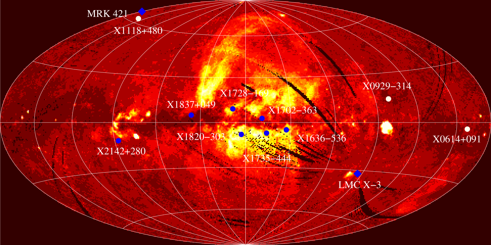
Figure 2: Directions of X-ray sources in the present study, shown on a ROSAT all-sky diffuse 3/4-keV-band intensity map (in the Aitoff projection; Snowden et al. 1997). These sources are the 10 LMXBs (filled circle) listed in Table 1, plus the two extragalactic sources, MRK 421 and LMC X–3 (filled diamond). The blue symbols represent those with significant absorption line detections, whereas the white symbols mark ones without a detection.

Table 1: Source Parameters

		($l$, $b$)	$D$	$z$	$P$	$A$
Source	Other Name	(deg)	(kpc)	(kpc)	(hr)	(R⊙)	Ref.
X1820–303	NGC 6624	(2.79, -7.91)	7.6	1.0	0.19	$<0.1$	1,2,3
X1728–169	GX 9+9	(8.51, 9.04)	5.0	0.8	4.2	1.6	1,4,5
X1837+049	Ser X–1	(36.12, 4.84)	8.4	0.7	13	$\sim$3.4	1,4
X2142+380	Cyg X–2	(87.33, -11.22)	7.2	1.4	235	26.9	1,9,15
X1118+480	$\cdots$	(157.66, 62.32)	1.8	1.6	4.1	$\cdots$	10, 11
X0614+091	$\cdots$	(200.88, -3.36)	$\leq 3$	$<0.2$	$\leq 1$	$\cdots$	12
X0929–314	$\cdots$	(260.11, 14.22)	$\geq 5$	$\geq 1.2$	0.72	$\cdots$	13,16
X1636–536	V801 Ara	(332.92, -4.82)	6.5	0.5	3.8	$1.6\pm 0.3$	1,4,7
X1735–444	V926 Sco	(346.05, -6.99)	7.1	0.9	4.6	$1.75\pm 0.02$	1,4,8
X1702–363	GX 349+2	(349.10, 2.75)	5.0	0.2	22	$\sim$4.8	14, 4

Note. — $D$, $z$, $P$, and $A$ are the distance, vertical distance away from the Galactic plane, orbit period, binary separation of the LMXBs.

Chandra carries two high spectral resolution instruments: the high energy transmission grating (HETG, Markert et al. 1995; Canizares et al. 2000) and the low energy transmission grating (LETG, Pease et al. 2002). The HETG consists of two grating assemblies, the high energy grating (HEG) and the medium energy grating (MEG). The LETG can be operated with either the advanced CCD imaging spectrometer (ACIS) or the high resolution camera (HRC), whereas the HETG works only with the ACIS. The energy resolution of the MEG, HEG, and LETG is 0.023, 0.012, and 0.05 Å (FWHM), respectively . For ease of reference, we show in Fig. 3 the effective area of the telescope/instruments as a function of photon wavelength. With the expected range of hot gas column density, the most promising absorption lines are at the wavelengths of $\sim 33$ Å (C VI), 20 Å (O VII and O VIII), and 13 Å (Ne IX and Ne X). The rest-frame line wavelengths are marked in Fig. 3. Note that the effective area of the LETG/ACIS is small at $\sim 33$ Å, where the cool gas absorption of the continuum is also severe. Furthermore, for a LETG/HRC spectrum, the higher order confusion could be severe at this wavelength and sorting orders may also cause some potential uncertainties. Therefore, the C VI is more difficult to detect than the other lines. The LETG/ACIS and LETG/HRC, with an effective area of $\sim 20$/30 cm² at 20/13 Å, should typically be the optimal combination for detecting O VII, O VIII, and Ne IX lines in one observation. The actual sensitivity of the LETG/ACIS also depends on the offset pointing, which determines where the source is placed on the detector and whether the lines are detected in the front-illuminated CCDs or the back-illuminated CCDs. For HETG observations, only the data from the MEG are considered here because it is substantially more sensitive than the HEG. Also because of the higher resolution of the MEG (by a factor of $\sim$ 2), it can be more sensitive for detecting narrow Ne IX and Ne X lines than the LETG.

Figure 3: The effective area of the first-order spectra of the HEG (dashed line), the MEG (solid line), the LETG/ACIS (dash-dotted line), and the LETG/HRC (dotted line; with unsorted orders). The vertical lines mark the rest frame wavelengths of highly ionized neon, oxygen, and carbon species considered in this work. The ACIS data were adopted from Chandra cycle 4.

Table 2: Chandra Observations

		Obs. Date		Exposure
Source	ObsID	(mm/dd/yy)	Grating/Detector	(ks)
X1820–303	98	03/10/00	LETG/HRC	15.12
	1021	07/21/01	HETG/ACIS	9.70
	1022	09/12/01	HETG/ACIS	10.89
X1728–169	703	08/22/00	HETG/ACIS	22.44
X1837+049	700	06/13/00	HETG/ACIS	78.06
X2142+380	87	04/24/00	LETG/HRC	30.16
	111	11/11/99	LETG/ACIS	6.2
	1016	08/12/01	HETG/ACIS	15.13
	1102	09/23/99	HETG/ACIS	28.98
X1118+480	1701	04/18/00	LETG/ACIS	27.83
X0614+091	100	11/28/99	LETG/HRC	26.23
X0929–314	3661	05/15/02	LETG/ACIS	17.96
X1636–536	105	10/20/99	HETG/ACIS	29.78
	1939	03/28/01	HETG/ACIS	27.06
X1735–444	704	06/09/00	HETG/ACIS	24.91
X1702–363	715	03/27/00	HETG/ACIS	10.98
	3354	04/09/02	HETG/ACIS	35.21

Among the 17 observations, only six (on five sources) used the LETG (Table 2). All of them, except for the short exposure on X2142+380 (ObsID 111, a calibration observation), have been analyzed for detecting absorption lines in previous studies. No significant highly ionized oxygen or neon absorption line is detected for X1118+480 (McClintock et al., 2001b), X0614+091 (Paerels et al., 2001), and X0929–314 (Juett et al., 2003). Our re-analysis of the data confirms this result. The detection of O VII K_α and K_β, O VIII K_α, and Ne IX K_α absorption lines has been reported for X1820–303, and an upper limit to the EW of the O VII absorption line has been set from the LETG spectrum of X2142+380 (Futamoto et al., 2004). Our analysis of these two sources used both LETG and HETG observations to achieve higher sensitivities. We report here for the first time the detection of the highly ionized absorption lines toward X1728–169, X1837+049, X1636–546, X1735–444, and X1702–363.

We re-process the observations, using the standard CIAO software (version 3.02) with the calibration database CALDB (version 2.25) to extract source and background spectra. For each observation we calculate the auxiliary response functions (ARFs) by running the CIAO thread fullgarf for the positive and the negative grating orders, and adopt the response matrix files (RMFs) from the CALDB directly. All the HETG/ACIS observations had the zeroth order images either severely piled-up or intentionally blocked to avoid telemetry saturation. We use the intersection of the two grating arms (both the HEG and the MEG) and the readout “streak” to determine the position of the source in the detector and to calibrate the wavelength of the grating spectra (e.g., Schulz et al. 2002). We then co-add the positive and the negative order spectra to improve the counting statistics. We further combine the spectra from multiple observations of a source, using the CIAO thread add_grating_spectra.

3 Implementation of an Absorption Line Model

Published X-ray absorption line analyses typically use the following procedure (e.g., Futamoto et al. 2004): (1) adopting a smooth function (e.g., a power-law) to characterize the spectral continuum and an additive negative Gaussian function to account for the absorption line profile; (2) fitting the observed spectrum to constrain the parameters of the functions; (3) using the fitted EW of the line in a curve-of-growth analysis to estimate the ionic column density. This procedure is simple but typically only adequate for individual unsaturated line analysis. The procedure also does not use all the information available in the observed spectrum: details of the observed line shape and/or the intrinsic connections between multiple lines. Although a joint analysis of the ionic column densities inferred from the analysis of individual lines can, in principle, be used to constrain the related physical parameters such as temperature and ionic abundances, it is generally difficult to correctly propagate the non-Gaussian errors of the estimated parameters.

We have implemented a general model (referred here as absline) for absorption line fitting in the X-ray spectral analysis software package XSPEC. Following the description of the absorption process given by Rybicki & Lightman (1979) and Nicastro et al. (1999), the radiation transfer at photon energy $\varepsilon$ can be expressed as

$$I(\varepsilon)=I_{c}(\varepsilon)e^{-\tau(\varepsilon)},$$ (1)

and

$$\tau(\varepsilon)=N_{i}\frac{\pi e^{2}}{m_{e}c}f_{lu}\phi(\varepsilon),$$ (2)

where $m_{e}$ is the electron mass, $c$ is the speed of light, and $f_{lu}$ is the oscillator strength of the electron transition from a lower level to an upper level. The ionic column density $N_{i}$ is a function of the reference element (hydrogen as the default) column density $N_{H}$ and the plasma temperature $T$,

$$N_{i}=N_{H}f_{a}f_{C}(T),$$ (3)

where $f_{a}$ is the corresponding element abundance relative to the reference element and $f_{C}(T)$ is the ionic fraction as a function of $T$ (assuming that the absorbing gas is in a CIE state). The normalized Voigt function $\phi(\varepsilon)$ is a convolution of the intrinsic Lorentz line profile with a Doppler broadening (assumed to be Gaussian):

$$\phi(\varepsilon) = \int^{+\infty}_{-\infty}\frac{\gamma}{4\pi^{2}(\varepsilon-\varepsilon_{l}-\Delta\varepsilon)^{2}+(\gamma/2)^{2}}\frac{e^{-(\Delta\varepsilon/\Delta\varepsilon_{D})^{2}}}{\sqrt{\pi}\Delta\varepsilon_{D}}d(\Delta\varepsilon)$$ (4)

$$= \frac{1}{\sqrt{\pi}\Delta\varepsilon_{D}}H(a,u),$$ (5)

$$H(a,u) = \frac{a}{\pi}\int^{+\infty}_{-\infty}\frac{e^{-y^{2}}}{(u-y)^{2}+a^{2}}dy~{},$$ (6)

where

$$a=\frac{\gamma}{4\pi\Delta\varepsilon_{D}},~{}~{}u=\frac{\varepsilon-\varepsilon_{l}}{\Delta\varepsilon_{D}}.$$ (7)

Here $\gamma$ is the natural broadening damping factor, $\varepsilon_{l}$ is the systemic (rest frame if redshift $z$=0) energy of the line, and $\Delta\varepsilon_{D}$ is the Doppler width

$$\Delta\varepsilon_{D}=\frac{b_{v}}{c}\varepsilon_{l},$$ (8)

in which

$$b_{v}=\left(\frac{2kT}{m_{i}}+\xi^{2}\right)^{1/2},$$ (9)

where $m_{i}$ is the ionic mass, $\xi$ is the velocity dispersion due to extra-broadening (e.g., turbulence). When $u$ is small (in the core region of a line), $H(a,u)\simeq e^{-u^{2}}$ gives a Gaussian profile, whereas when $u$ is large (in the wings of a line) $H(a,u)\simeq a/\pi u^{2}$ is close to a Lorentz profile.

We define $e^{-\tau(\varepsilon)}$, part of Eq. 1, as our multiplicative absline model, which is specified by five parameters: the plasma temperature $T$, central line energy $\varepsilon_{l}$, ion velocity dispersion $b_{v}$, the hot-phase hydrogen column density $N_{H}$ (or $N_{i}$ for a chosen ion), and the metal abundance $f_{a}$. Other parameters ($f_{lu}$ and $\gamma$) are given for a specific line (Table 3). While $\varepsilon_{l}$ is very sensitive to the line centroid in a fit, $b_{v}$ and $N_{i}$ can be constrained by the shape and intensity of the line. When multiple lines are present, one can conduct a joint fit, which may also allow for the estimation of $T$, $N_{H}$, and/or $f_{a}$ and their uncertainties.

Table 3: Absorption Line Parameters

	rest $\lambda/\varepsilon_{l}$		$\gamma$
Line	(Å/eV)	$f_{lu}$	($10^{-2}$ eV)
Ne X Kα	12.134/1021.79	0.416	2.61
Ne IX Kα	13.448/921.95	0.657	3.35
O VII Kβ	18.629/665.55	0.146	0.39
O VIII Kα	18.967/653.69	0.277	1.06
O VII Kα	21.602/573.95	0.696	1.37

Note. — The $f_{lu}$ is the transition oscillator strength and $\gamma$ is the natural broadening damping factor. The values of Ne IX are adopted from Behar & Netzer (2002) and the others from Verner et al. (1996).

Note that in the absline model, $b_{v}$ is used as an independent parameter (not constrained by Eq. 9), and can be smaller than the CIE thermal broadening $(2kT/m_{i})^{1/2}$. Therefore, with the adopted Voigt function, the absline model can be applied as well to a photo-ionized plasma where $b_{v}\simeq 0$. The inclusion of the Lorentz profile in calculating the line profile is important when the Doppler broadening is small (e.g., in an over-cooled or photo-ionized plasma) and/or when the column density is large. Using the Lorentz profile alone gives a firm upper limit to the ionic column density (e.g., Futamoto et al. 2004).

Fig. 4 illustrates the difference between the additive Gaussian and the absline models. The additive Gaussian model is a good approximation to the absline model only when $\tau_{0}$ is small ($\lesssim 1$). When $\tau_{0}$ is large ($>1$), the additive Gaussian profile deviates significantly from the absline profile and the inferred velocity dispersion $b_{G}$, for example, can be substantially overestimated.

Figure 4: Comparison between the absline model of a Ne IX K_α absorption line (solid line) and the best-fit additive Gaussian model (dotted). The absline model assumes a velocity dispersion $b_{v}$=45 km s^-1 (thermal velocity at T$\sim 2.4\times 10^{6}$ K) as well as ${\rm log(N_{NeIX})}$=15.0, 15.5, 16.0, and 16.5 cm^-2 (for the panels from left to right), corresponding to optical depths of $\tau_{0}=$0.29, 0.91, 2.89, and 9.10 at the line centroid (921.95 eV $\sim$ 13.448 Å). The $b_{v}=0$ Lorentz profiles (dashed) are also shown for reference in the panels. The limitations of the additive Gaussian model are characterized by the best fit $b_{G}$ values as they significantly differ from $b_{v}$=45 km s^-1.

4 Analysis and Results

Our absorption line analysis is based on the data in 12–14, 18–20, and 20–22 Å bandpasses, which embrace the Ne X K_α and Ne IX K_α, O VII K_β and O VIII K_α, and O VII K_α lines, respectively (Table 3). The chosen band width (2 Å) is a compromise between maximizing the counting statistics and reducing the effect of the potential deviation of the spectral continuum from our power-law characterization. The subtracted background contributes $\leq 5$% to the source counts in the wavelength bandpasses for all sources. We apply both the commonly used additive Gaussian model and the new absline model to the absorption line analysis of the 10 selected sources (Tables 1-2). The models, including both the continuum and the line(s), are convolved with the instrument responses in XSPEC (version 11.3.1) before they were fitted to the observations. We choose the signal-to-continuum-noise ratio $S/N=3\sigma$ (corresponding to a false detection probability $\sim 0.1\%$) as the detection threshold. Seven sources show significant Ne IX K_α absorption lines in the MEG spectra; three of these sources also show O VII K_β, O VIII K_α, and/or O VII K_α absorption line(s). The O VII K_α absorption line is not significant in the LETG/HRC spectrum of X2142+380, which is consistent with the previous work by Futamoto et al. (2004), but we detect significant Ne IX K_α and O VII K_β absorption lines in the more sensitive MEG spectra. All the detected lines are unresolved at 90% confidence level. The lack of significant absorption lines in the spectra of X1118+480, X0614+091, and X0929–314 is consistent with the results from the previous studies as mentioned in §2. No Ne X K_α absorption line is detected in any of the 10 sources.

For the detection of individual lines, it is convenient as a first pass to use the Gaussian model. We estimate the line centroid energy and EW for each detected line. Fig. 5 shows the Gaussian model fits to the Ne IX K_α lines. For each sight-line, we also estimate an upper limit to the EW of the Ne X K_α line by fixing its line centroid energy at the rest frame energy and jointly fitting its width with the Ne IX K_α line.

Figure 5: The Ne IX K_α absorption lines in the spectra of the 10 sources. The solid line in each panel represents a Gaussian plus power-law model folded with the instrumental response; the vertical dashed line marks the rest frame wavelength of the line. The apparent broad line features in (d), (e), and (g), are partly due to dip in the instrument effective area near the line central wavelength; the short vertical arrows indicate other instrumental features. The bin size is 12.5 mÅ for LETG observations (panels e, f, g) and is 5.0 mÅ for HETG observations (the other panels).

Using the absline model, we jointly fit multiple lines of each source. Table 4 marks the included lines. In such a fit, we link the model parameters $b_{v}$, $T$, and $N_{H}$ of the lines; the slight dependence of $b_{v}$ on the different ion mass is neglected ($<5$ km s^-1; see Eq. 9). Because of the limited number and quality of the line detections, we use a fixed ISM abundance (Wilms et al., 2000) and assume the CIE for the X-ray-absorbing gas. For those lines that are not detected, we fix $\varepsilon_{l}$ to their rest-frame energies. Fig. 6 presents the velocity profiles of the jointly-fitted multiple lines.

Figure 6: The velocity profiles of the joint-fitted absorption lines. The transition and centroid wavelength of each line as well as the used instrument are listed in each panel. The solid histogram of each panel represents the best-fit absline-modified power-law model folded with the instrumental response. The vertical dashed line marks the zero velocity. A negative velocity indicates a blue shift. The bin sizes are the same as in Fig. 5.

Figure 6: Continued.

Figure 6: Continued.

Our results are summarized in Table 4. The sources X1118+480, X0614+091, and X0929–314 are not included in the table; their poor data quality (in terms of both counting statistics and spectral resolution) does not give any meaningful upper limits to either EWs or the ionic column densities. The $\varepsilon_{l}$ values and their uncertainties constrained from absline model are consistent with those obtained from the Gaussian model and are thus not repeatedly presented in the table. In addition to setting the upper limits to $b_{v}$ from the observed lines, the joint-fits further constrain the lower bounds on $b_{v}$ for four of the sources (Table 4). If $b_{v}$ were smaller, the (unresolved) line would then be deeper in order to provide the same observed absorption. The degree of saturation $\tau_{0}$ varies among the jointly-fitted lines and therefore affects their relative strengths, which sets a lower bound on $b_{v}$. Table 4 further includes a hot gas hydrogen density $n_{H}$, estimated from assuming a uniform distribution with a unity filling factor along each sight-line.

Table 4: Results of Gaussian and absline model fits

			Gaussian model			absline model
		S/N	$cz$	$b_{G}$	EW		$b_{v}$	log(T)	${\rm log(N_{H})}$	${\rm n_{H}}$	log(${\rm N_{NeIX}^{p}}$)
Source	Line	($\sigma$)	(km/s)	(km/s)	(eV)	Joint	(km/s)	(K)	(cm-2)	(10-3cm-3)	(cm-2)
X1820–303	Ne X Kα	$<1$	$\cdots$	$\cdots$	$<0.09$	$\surd$
	Ne IX Kα	8.6	-89(-112, 89)	$<$346	0.43(0.28, 0.63)	$\surd$
	O VII Kβ	$<1$	$\cdots$	$\cdots$	$\cdots$	$\surd$
	O VIII Kα	6.0	-86(-201, 152)	$<$490	0.65(0.34, 0.98)	$\surd$
	O VII Kα	10.6	175(-120, 125)	$<$347	0.58(0.41, 0.79)	$\surd$
							191(62, 346)	6.4(6.2, 6.5)	20.0(19.8, 20.2)	4.3(2.7, 6.8)	$<$18.54
X1728–169	Ne X Kα	$<1$	$\cdots$	$\cdots$	$<0.36$	$\surd$
	Ne IX Kα	4.9	-134(-223, 134)	$<$532	0.30(0.14, 0.52)	$\surd$
	O VII Kβ	2.0	-261(-342, 264)	$<$375	0.39(0.14, 0.65)	$\surd$
	O VIII Kα	2.1	178(-298, 617)	$<$531	0.43(0.16, 0.70)	$\surd$
							$<375$	6.3(6.0, 6.5)	19.9(19.7, 22.2)	5.1(3.2, 1027)	$<$18.37
X1837+049	Ne X Kα	$<1$	$\cdots$	$\cdots$	$<0.11$	$\surd$
	Ne IX Kα	9.9	22(-89, 89)	$<$366	0.42(0.37, 0.47)	$\surd$
	O VII Kβ	$<1$	$\cdots$	$\cdots$	$\cdots$	$\surd$
	O VIII Kα	$<1$	$\cdots$	$\cdots$	$\cdots$	$\surd$
							280(111,443)	6.45(6.37, 6.54)	20.1(19.9, 20.2)	4.8(3.1, 6.1)	$<$18.46
X2142+380	Ne X Kα	$<1$	$\cdots$	$\cdots$	$<0.11$	$\surd$
	Ne IX Kα	4.8	-223(-267, 290)	$<$797	0.25(0.14, 0.40)	$\surd$
	O VII Kβ	4.9	1(-263, 285)	$<$369	0.24(0.01, 0.41)	$\surd$
	O VIII Kα	$<1$	$\cdots$	$\cdots$	$\cdots$	$\surd$
	O VII Kα	$<1$	$\cdots$	$\cdots$	$\cdots$
							383(30, 664)	6.3(6.2, 6.4)	19.7(19.5, 19.9)	2.3(1.4, 3.6)	$<$18.10
X1636–536	Ne X Kα	$<1$	$\cdots$	$\cdots$	$<0.09$	$\surd$
	Ne IX Kα	8.4	-67(-44, 45)	$<$213	0.38(0.27, 0.49)	$\surd$
	O VII Kβ	$<2$	$\cdots$	$\cdots$	$\cdots$	$\surd$
	O VIII Kα	$<2$	$\cdots$	$\cdots$	$\cdots$	$\surd$
							$<$105	6.3(5.7, 6.8)	20.2(19.5, 22.3)	7.9(1.6, 995)	$<$18.28
X1735–444	Ne X Kα	$<1$	$\cdots$	$\cdots$	$<0.31$	$\surd$
	Ne IX Kα	9.0	-22(-156, 200)	$<$724	0.78(0.44, 0.84)	$\surd$
	O VII Kβ	$<2$	$\cdots$	$\cdots$	$\cdots$	$\surd$
	O VIII Kα	3.8	-168(-611, 375)	$<$746	$<$0.90	$\surd$
							369(58, 638)	6.5(6.3, 6.6)	20.2(20.0, 20.4)	7.2(4.6, 11)	$<$18.84
X1702–363	Ne X Kα	$<1$	$\cdots$	$\cdots$	$<0.28$	$\surd$
	Ne IX Kα	5.5	-201(-289, 335)	$<$593	0.50(0.17, 0.60)	$\surd$
	O VIII Kβ	$<1$	$\cdots$	$\cdots$	$\cdots$	$\surd$
	O VIII Kα	$<1$	$\cdots$	$\cdots$	$\cdots$	$\surd$
							$<$899	6.0(5.6, 7.1)	19.9(19.4, 20.3)	5.1(1.6, 13)	$<$18.62

Considering the potential uncertainties in the systematics of the spectral resolution calibration, we have also estimated the Ne IX column density ${\rm N_{NeIX}^{p}}$ by fitting individual Ne IX K_α lines with the natural broadening only (§3). This “firm” upper limit to the Ne IX column density is presented in the last column of Table 4.

The joint-fits give direct estimates of $N_{H}$ and $T$, although the uncertainties are large along some sight-lines. We define a mean measurement $\overline{p}$ and its 90% upper and lower uncertainties $\Delta\overline{p}_{\pm}$ of a parameter as

$$\overline{p}=\frac{\sum_{i=1}^{7}p_{i}/\sigma^{2}_{i}}{\sum_{i=1}^{7}1/\sigma^{2}_{i}},~{}~{}\Delta\overline{p}_{\pm}=\left(\sum_{i=1}^{7}\frac{1}{\Delta p^{2}_{\pm i}}\right)^{-1/2},~{}~{}{\rm and}~{}~{}\sigma^{2}_{i}=\Delta p^{2}_{+i}+\Delta p^{2}_{-i},$$

where $p_{i}$, $\Delta p_{+i}$ and $\Delta p_{-i}$ are the measurement and its corresponding 90% upper and lower uncertainties along the $i$th sight-line with the absorption line(s) detected. We obtain $\overline{T}=2.4(2.1,2.7)\times 10^{6}$ K, $\overline{N}_{H}=8(6,10)\times 10^{19}$ cm^-2, and $\overline{n}_{H}=3.6(3.0,4.5)\times 10^{-3}$ cm^-3.

The plasma properties along the sight-line of X1820–303 are mostly consistent with those obtained by Futamoto et al. (2004) from a curve-of-growth analysis. However, they prefer a large $b_{v}$ ($\geq$ 200 km s^-1), arguing that otherwise the inferred $N_{H}$ would be comparable to, or even larger than, the neutral hydrogen column density observed in the field. Our $b_{v}$ value can be as low as 62 km s^-1, and the hot gas column density is well below the neutral hydrogen column density of $1.9\times 10^{21}$ cm^-2 (Bohlin, Savage, & Drake, 1978). This discrepancy is probably due to a significant deviation of their used additive Gaussian model from the proper multiplicative absline profile (Fig. 4) and to the inaccurate error propagation of the temperature in their analysis (§3).

5 Origin of the Hot Gas

In principle, the X-ray-absorbing hot gas could be local to the binary systems. To account for the large column densities estimated above, a plausible scenario might be the photo-ionized winds from the accretion disks that are presumably responsible for the X-ray continuous emission. Such a scenario, if confirmed, would be interesting in its own right. However, we find that it has serious difficulties:

• An absorption line produced in an accretion disk wind should be blue-shifted and broadened with a magnitude comparable to the escape speed of the accreting compact object (e.g., Ueda et al. 2004). The line shift, for example, can be characterized by $\Delta\lambda/\lambda_{0}=v_{w}/c\sim(2r_{g}/r_{l})^{1/2}$, where $v_{w}$ is the wind velocity, $r_{l}$ is the starting radius where the absorption line is produced, $r_{g}=GM/c^{2}$ is the gravitational radius. Since all the detected X-ray absorption lines are consistent with $cz\approx 0$, using the wavelength accuracy 0.011Å of MEG as $\Delta\lambda$ and assuming the compact object mass $M=1.4M_{\odot}$, we obtain $r_{l}\gtrsim 9~{}R_{\odot}$. This required $r_{l}$ value is much greater than the binary separation $A$ (Table 1) for all the sources with absorption lines detected except for X2142+380.

• The Ne IX absorption should arise only in a region with a proper ionization state. If the electron density in the wind can be approximated as $n(r)\propto 1/r^{\alpha}$ ($\alpha>1$), the ionization parameter can then be written as,

  $$U\equiv L_{X}/\left[n(r)r^{2}\right]=L_{X}r^{\alpha-2}/\left[N_{H}(\alpha-1)r_{l}^{\alpha-1}\right],$$

  where $r>r_{l}$. According to Kallman & McCray (1982), Ne IX is the dominant ionization state of neon only when log($U$)$\leq 2$ in both optical thin and thick cases. We estimate the luminosity of the individual sources to be in the range of $2-7\times 10^{37}{\rm ergs~{}s^{-1}}$ (assuming the source distances in Table 1). Further assuming a Ne IX fraction $\sim$ 0.5 and taking $N_{H}\sim 10^{23}$ cm^-2 (corresponding to the maximum value of the ${\rm N_{NeIX}^{p}}$; Table 4), $\alpha=2$ (constant wind velocity), we obtain $r_{l}\geq 7.5~{}R_{\odot}$. Again, the required $r_{l}$ is much larger than the binary separation $A$ of all the sources except for X2142+380.

• We should also expect additional signatures of the wind. If the wind is launched at a radius $r_{w}$ away from the compact object, the hot hydrogen column density between $r_{w}$ and $r_{l}$ is then $N_{w}=N_{H}\left[(r_{l}/r_{w})^{\alpha-1}-1\right]$, where $N_{H}$ is inferred from the X-ray absorption lines. Taking $r_{w}=2\times 10^{8}$ cm (corresponding to $\sim 10^{3}~{}r_{g},3\times 10^{-3}R_{\odot}$; Li & Wang 1999), $r_{l}\sim 10R_{\odot}$, and $\alpha=2$, we got $N_{w}\sim 10^{3}N_{H}$. Such a wind should then result in strong emission lines, which are, however, absent in the spectra of the sources. Furthermore, because the ionization state should increase with decreasing radius, we should observe a column density of Ne X comparable to, or greater than, that of Ne IX. But we do not detect any significant Ne X absorption line in any of the spectra.

Based on these arguments, even though not conclusive (there are other possibilities such as a clumpy wind), we find that the X-ray line absorption is unlikely to be associated with the LMXBs. An interstellar origin of the absorption is most likely and is assumed in the following discussion.

6 Spatial Distribution of the Hot Gas

To tighten the constraints on the distribution of the X-ray-absorbing gas, we include the results from the absorption line study of the X-ray binary LMC X–3 (Wang et al., 2005) and an AGN MRK 421 (Yao et al., 2005). The $N_{H}$ measurements, as listed in Table 5, are made in the same way as the 7 Galactic LMXBs reported above. With this set of 9 column density measurements, though still quite sparse, we attempt to characterize the overall spatial scale of the X-ray-absorbing gas, by assuming two extreme distribution geometry, an infinite disk or a sphere.

Table 5: Results of the Sight-lines toward Extragalactic Sources

	($l,b$)	D	${\rm log(N_{H})}$
Source	(deg)	(Mpc)	(cm-2)
LMC X–3	(273.58, -32.08)	0.05	19.7(19.2, 20.5)
MRK 421	(179.83, 65.03)	118	19.4(19.3, 19.6)

Note. — The O VII K_α line is only searched in the spectra of LETG observations (Table 2). A negative $cz$ value indicates a blue shift. In a Gaussian model fit, $b_{G}$ is $\sqrt{2}$ times the standard deviation (mimicking the velocity dispersion $b_{v}$ in an absline model fit). The “Joint” column marks those absorption lines utilized in the joint-fits with the absline model. The n_H is the averaged hot gas density derived from the column density N_H divided by the source distance $D$ listed in Table 1. All limits are at the 90% confidence level. See the text for details.

Note. — The $N_{H}$ values were adopted from Wang et al. (2005) and Yao et al. (2005) respectively. The distance to MRK 421 was calculated by assuming ${\rm H_{0}=75~{}km~{}s^{-1}~{}Mpc^{-1}}$.

For the disk distribution, we assume

$$n(z)=n_{0}e^{-|z|/z_{h}},$$ (10)

where $n_{0}$ is the mean gas density at the Galactic plane and $z_{h}$ is the vertical scale height. The column density can then be expressed as

$$N_{H}=n_{0}z_{h}(1-e^{-|z|/z_{h}})/\sin|b|.$$ (11)

A $\chi^{2}$ fit to the data (Fig. 7) gives $n_{0}=6.4(4.7,8.8)\times 10^{-3}{\rm cm^{-3}}$ and $z_{h}$=1.2(0.7, 2.2) kpc with the best-fit $\chi^{2}/d.o.f.=7.2/7$. Here, we have set the $|z|$ value of MRK 421 to be $\sim$100 kpc for ease of fitting and plotting; the exact value is irrelevant as long as it is much larger than $z_{h}$. Furthermore, the 90% confidence uncertainties of the individual $N_{H}$ measurements have been scaled by a factor of 0.61 to mimic the required 1 $\sigma$ errors in the $\chi^{2}$ fit.

Figure 7: Left panel: The vertical hot gas column density as a function of the distance from the Galactic plane. Diamonds mark the measurements toward the LMXBs and triangles represent the line-of-sights to the extragalactic sources (see the text for details). The dashed line is the best-fit exponential function with $n_{0}=6.4\times 10^{-3}{\rm cm^{-3}}$ and $z_{h}=1.2{\rm~{}kpc}$ (Eq. 11). Right panel: $z_{h}$ vs. $n_{0}$ confidence contours at the 68%, 90%, and 99% confidence levels.

For the spherical distribution, we assume

$$n(R)=n_{c}\left[1+(R/R_{h})^{2}\right]^{-1},$$ (12)

adopted from the so-called $\beta$-model $n(R)=n_{c}\left[1+(R/R_{h})^{2}\right]^{-3\beta/2}$ with $\beta=2/3$ (Sarazin, 1988; Jones & Forman, 1984), where $n_{c}$ is the hot gas density at the Galactic center (GC) and $R_{h}$ is the scale radius. The hot gas column density toward a source with Galactic coordinates ($l$, $b$) and a distance $D$ (Fig. 8) can be calculated via the following integration,

$$N_{H} = \int^{D}_{0}n_{c}\left[1+\left(\frac{R}{R_{h}}\right)^{2}\right]^{-1}dr$$ (13)

$$= n_{c}\int^{D}_{0}\left[1+\frac{r^{2}+R_{0}^{2}-2rR_{0}\cos\theta}{R_{h}^{2}}\right]^{-1}dr$$ (14)

$$= n_{c}R_{h}\int^{\frac{D-R_{0}\cos\theta}{R_{h}}}_{-\frac{R_{0}\cos\theta}{R_{h}}}\left(a^{2}+x^{2}\right)^{-1}dx$$ (15)

$$= \frac{n_{c}R_{h}}{a}\left[\tan^{-1}\left(\frac{D-R_{0}\cos\theta}{aR_{h}}\right)-\tan^{-1}\left(\frac{-R_{0}\cos\theta}{aR_{h}}\right)\right],$$ (16)

where $a^{2}=1+{R_{0}^{2}\sin^{2}\theta}/{R_{h}^{2}}$, $x=({r-R_{0}\cos\theta})/{R_{h}}$, $R_{0}$ is the distance between the Sun and GC (taken as 8 kpc in this work), and $\theta$ is the angular separation between GC and the source ($\cos\theta=\cos l\cos b$). The fit ($\chi^{2}/d.o.f=9.4/7$) of the data with this model (Fig. 9) is slightly worse than that with the disk model. The best-fit parameters are $n_{c}=6.2(4.1,10.0)\times 10^{-3}$ cm^-3, $R_{h}=2.3(1.2,3.9)$ kpc.

Figure 8: Geometry for the Galaxy-centered spherical distribution of the X-ray-absorbing hot gas.

Figure 9: Left panel: The total hot gas column density $N_{H}^{T}$ as a function of the off-GC impact radius $R_{p}$ in the spherical distribution model. $N_{H}^{T}$ is calculated via an integration along the dotted line (i.e., $r=-\infty$ to $\infty$) in Fig. 8. The column density measurements and their errors have been enlarged by the ratio of $N_{H}^{T}$ to the model $N_{H}$ between the Sun and the source (see Fig. 8). This plot is for demonstration only; the actual fit is based on the comparison between the measured and modeled $N_{H}$ values. The meaning of the symbols is the same as that in Fig. 7. The dashed line represents the best fit function with $n_{c}=6.2\times 10^{-3}$ cm^-3, $R_{h}=2.3$ kpc (Eq. 16). Right panel: $R_{h}$ vs. $n_{c}$ contour at the 68%, 90%, and 99% confidence levels.

With the fitted $n_{0}$ and $z_{h}$, or $n_{c}$ and $R_{h}$, we estimate the total hot gas mass as $\sim 2.7\times 10^{8}$ M_⊙ and $\sim 1.2\times 10^{8}$ M_⊙ for the disk and the sphere characterizations within a 15 kpc radius. This mass estimate is very uncertain as it depends sensitively on the assumed characterization forms and their spatial limits, which cannot be constrained by the existing data. Taking the CIE radiative cooling function ${\rm\sim 5\times 10^{-23}~{}ergs~{}cm^{3}~{}s^{-1}}$ at $T\sim 2.4\times 10^{6}$ K (Sutherland & Dopita, 1993), we obtain the corresponding cooling rates as ${\rm\sim 5\times 10^{40}~{}ergs~{}s^{-1}}$ and ${\rm\sim 7\times 10^{39}~{}ergs~{}s^{-1}}$, which, within their uncertainties, are comparable to those obtained from observations of nearby disk galaxies of similar sizes (e.g., Wang et al. 2003). The cooling probably accounts for only a small fraction of the expected supernova (SN) mechanical energy input in the Galaxy (${\rm\sim 10^{42}~{}ergs~{}s^{-1}}$, assuming $10^{51}~{}{\rm ergs}$ per SN and one SN per 30 years).

A more realistic spatial distribution of the hot gas may be between the above two extreme characterizations. Also our model fits are probably quite biased because of the limited number of the sight-lines. Nevertheless, the fitted values of $z_{h}$ and $R_{h}$ consistently indicate a small scale of the hot gas distribution. Because the fits incorporate the measurements toward the two extragalactic sources, this small scale suggests that a bulk of the highly-ionized X-ray-absorbing gas arises from regions close to the Galactic disk.

In this work, we adopt the element abundances from Wilms et al. (2000) in which the abundance ratios of O/H and Ne/H are 0.58 and 0.71 times solar values given by Anders & Grevesse (1989). The real ISM abundances are still very uncertain (e.g., Savage & Sembach 1996). However, if the real abundances are smaller or larger by a factor than those we adopted, the derived $N_{H}$ (in §4), $n_{0}$, $n_{c}$, and the total mass of the hot gas will be larger or smaller by the same factor accordingly, while the inferred $T$ (in §4), $z_{h}$, and $R_{h}$ are still valid. Since the Ne IX and the O VII/O VIII absorption lines are used here as the diagnostic of the ionization states and the gas temperature (Table 4), the results depend on the assumed Ne/O abundance ratio. However, this dependence can be partially compensated by a change in the best-fit $T$ (please refer to Fig. 1). Therefore, the $N_{H}$ measurements should not be very sensitive to the assumed Ne/O ratio. In general, both $T$ and Ne/O could be constrained simultaneously if multiple high S/N absorption lines of these two elements are available (§1).

7 Comparisons with O VI Absorption and X-ray Emission Measurements

We compare the above results from the X-ray absorption lines with those from observations of Galactic far-UV O VI absorption lines and diffuse soft X-ray emission. Although the O VI absorption doublet (1031.93 and 1037.62 Å) has commonly been detected in the spectra of both extragalactic and Galactic sources, the nature of the absorbing gas is still very uncertain. The O VI population peaks at $T\sim 3\times 10^{5}$ K, near the peak of the cooling curve of a CIE plasma. Therefore, such intermediate-temperature gas is expected primarily at the interfaces between the cool/warm clouds and the hot gas, consistent with the finding that about half of distinct high-velocity O VI absorbers have H I counterparts (Sembach et al., 2003). The bulk of the observed Galactic O VI density can be well described as a patchy exponential distribution with a scale height between 2.3 and 4 kpc (e.g., Zsargó et al. 2003). This scale height is greater than that inferred from our disk modeling of the X-ray absorption lines, which may indicate an evolutionary sequence of the hot gas.

The X-ray-absorbing gas should also be responsible for some of the O VI population. We use the constrained $n_{0}$ and the CIE ionization fraction of O VI at $T\sim 2.4\times 10^{6}$ K to estimate the O VI midplane density as 2.6(1.9, 3.5) $\times 10^{-9}$ cm^-3, which is $\sim 1/7$ of the value obtained from an O VI survey (Jenkins et al., 2001). Therefore, a significant fraction of the O VI absorption could arise from the X-ray-absorbing hot gas. Interestingly, the tightly constrained mean velocity dispersion of the O VI-absorbing gas (Savage et al., 2003; Zsargó et al., 2003) agrees well with the oxygen thermal velocity ($\sim 50$ km s^-1) at $T\sim 2.4\times 10^{6}$ K, but is substantially greater than the velocity ($\sim 18$ km s^-1) at the O VI peak temperature. Of course, much of the O VI line velocity dispersion may arise from turbulent and/or differential motion (e.g., due to the circular rotation of the disk and halo of the Galaxy). Detailed cross-correlation between the O VI and X-ray absorbing gas along individual sight-lines may provide insights into the connection between the O VI- and X-ray-absorbing gases.

Fig. 2 shows a ROSAT all-sky diffuse 3/4-keV background map, including the locations of our studied sources and the two extragalactic sources. Among the seven LMXBs with the detected X-ray absorption lines (Table 4), five (X1820–303, X1728–169, X1636–536, X1735–444, and X1702–363) are within a $30^{\circ}$ radius of the GC; in this Galactic inner region, the diffuse SXB is greatly enhanced in both 3/4 and 1.5 keV bands. The bulk of this enhancement may arise from the Galactic bulge (e.g., Wang 1998; Almy et al. 2000). The three sources (X1118+480, X0614+019, and X0929–314), in which no absorption line is detected, are all toward outer Galactic regions with relatively low SXB emission; X1118+480 and X0614+019 are also very close to us. Our estimated temperature and density of the X-ray-absorbing hot gas are between those inferred from the modeling of the X-ray emission gas in the solar neighborhood and the Galactic bulge (Wang, 1998; Kuntz & Snowden, 2000). These apparent correlation and consistency suggest that the absorption lines and the SXB emission arise from the same hot gas.

8 Summary and Conclusions

We have systematically searched for absorption lines produced by highly ionized species (O VII, O VIII, and Ne IX) in the spectra of 10 LMXBs observed with Chandra grating instruments. Much of our analysis is based on the multiplicative absorption line model, absline , which we have constructed to allow for both an accurate absorption line profile fit and a joint analysis of multiple line transitions from same and/or different ions in a CIE plasma.

We detect significant Ne IX K_α absorption lines in seven of the 10 LMXBs. Three of these seven sources also show evidence for absorption by O VII K_α, K_β, and/or O VIII K_α. The detected absorption lines most likely originate in the intervening diffuse hot gas, rather than in the LMXBs themselves, because of the absence of the expected line centroid shift and broadening as well as the lack of significant Ne X absorption and emission lines, which may be expected from a disk wind. We estimate the average temperature and the hydrogen density of the absorbing gas to be $\sim 2\times 10^{6}$ K and $\sim 4\times 10^{-3}$ cm^-3, under the assumptions of the CIE, unity filling factor, and ISM abundances.

The hot gas is apparently located in and around the Galactic disk and preferentially in inner regions of the Galaxy, consistent with the distribution of the diffuse SXB. We have included the column density measurements inferred from the absorption lines detected in two extragalactic sources to constrain the global distribution of the X-ray-absorbing hot gas. Modeled with an infinite disk with an exponential vertical distribution, the gas has a midplane density of $\sim 6\times 10^{-3}$ cm^-3 and a scale height of $\sim 1$ kpc. The gas, if indeed in a CIE state, can account for $\sim$ 1/7 of the O VI absorption observed in the Galaxy. Modeled with a spheric radial distribution, the X-ray-absorbing hot gas has a predicted density of $\sim 6\times 10^{-3}$ cm^-3 at the GC and a core radius of $\sim 2$ kpc. But this spherical model gives a less satisfactory fit than the disk characterization. The small characteristic scales indicate that the bulk, if not all, of the $cz\sim 0$ X-ray-absorbing hot gas detected in extragalactic sources to date is of Galactic origin.

While far-UV absorption and X-ray emission studies have had a long history, X-ray absorption spectroscopy of the Galactic diffuse hot gas has just begun. Nevertheless, the results presented above demonstrate the potential of X-ray absorption line spectroscopy as a powerful diagnostic tool for probing the hot gas in our Galaxy.

References

- Almy et al. (2000) Almy, R. G., et al. 2000, ApJ, 545, 290
- Anders & Grevesse (1989) Anders, E., & Grevesse, N. 1989, Geochim. Cosmochim. Acta, 53, 197
- Arnaud & Rothenflug (1985) Arnaud, M., & Rothenflug, R. 1985 A&AS, 60, 425
- Behar & Netzer (2002) Behar, E., & Netzer, H. 2002, ApJ, 570, 165
- Bohlin, Savage, & Drake (1978) Bohlin, R. C., Savage, B. D., & Drake, J. F. 1978, ApJ, 224, 132
- Brandt et al. (1992) Brandt, S., et al. 1992, A&A, 262, L15
- Canizares et al. (2000) Canizares, C. R., et al. 2000, ApJ, 539, L41
- Christian & Swank (1997) Christian, D., & Swank, J. 1997, ApJS, 109, 177
- Cook et al. (2000) Cook, L., Patterson J., Buczynski, D., & Fried, R. 2000, IAUC, 7397, 2
- Cox & Smith (1974) Cox, D. P., & Smith, B. W. 1974, ApJ, 189, 105.
- Cowley et al. (1979) Cowley, A. P., Crampton, D., & Hutchings, J. B. 1979, ApJ, 231, 539
- Fang et al. (2002) Fang, T., et al. 2002, ApJ, 572, 127
- Fang et al. (2003) Fang, T., Sembach, K. R., & Canizares, C. R. 2003, ApJ, 586, 49
- Ferriére (1998) Ferriére, K. 1998, ApJ, 497, 759
- Futamoto et al. (2004) Futamoto, K., et al. 2004, ApJ, 605, 793
- Galloway et al. (2002) Galloway, D. K., et al. 2002, ApJ, 576, L137
- Heiles (1987) Heiles, C. 1987, ApJ, 315, 555
- Homer et al. (1996) Homer, L., et al. 1996, MNRAS, 282, L37
- Jansen et al. (2001) Jansen, F., et al. 2001, A&A, 365, L1
- Jenkins et al. (2001) Jenkins, E. B., Bowen, D. V., & Sembach, K. R. 2001, in Proc. XVIIth IAP Colloq. Gaseous Matter in Galactic and Intergalactic Space, ed. R. Ferlet, M. Lemoine, J. M. Desert, & B. Raban (Paris: Frontier Group), 99
- Jimenez-Garate et al. (2002) Jimenez-Garate, M., et al. 2002, ApJ, 578, 391
- Jones & Forman (1984) Jones, C., & Forman, W. 1984, ApJ, 276, 38.
- Juett et al. (2003) Juett, A., Galloway, D., & Chakrabarty, D. 2003, ApJ, 587, 754
- Juett et al. (2004) Juett, A., Schulz, N., & Chakrabarty, D. 2004, ApJ, 612, 308
- Li & Wang (1999) Li, X.-D., & Wang, Z.-R. 1999, ApJ, 513, 845
- Kallman & McCray (1982) Kallman, T. R., & McCray, R. 1982, ApJS, 50, 263
- Kuntz & Snowden (2000) Kuntz, K. D., & Snowden, S. L 2000, ApJ, 543, 195
- Kuulkers et al. (2003) Kuulkers, E., et al. 2003, A&A, 399, 663
- Lawrence et al. (1983) Lawrence, A., et al. 1983, ApJ, 271, 793
- Markert et al. (1995) Markert, T. H., et al. 1995, Proc. SPIE, 2280, 168
- Markwardt et al. (2002) Markwardt, C. B., et al. 2002, ApJ, 575, L21
- McCammon et al. (2002) McCammon, D., et al. 2002, ApJ, 576, 188
- McClintock et al. (2001a) McClintock, J. E., et al. 2001, ApJ, 551,L147
- McClintock et al. (2001b) McClintock, J. E., et al. 2001, ApJ, 555,477
- McKee & Ostriker (1977) McKee, C. F., & Ostriker, J. P. 1977, ApJ, 218, 148
- Miller et al. (2004) Miller, J., et al. 2004, ApJ, 601, 450
- Nicastro et al. (1999) Nicastro, F., Fiore, F, & Matt, G. 1999, ApJ, 517, 108
- Nicastro et al. (2002) Nicastro, F., et al. 2002, ApJ, 573, 157
- Nicastro (2003) Nicastro, F. 2003, (astro-ph/0311162)
- Paczynski (1971) Paczynski, B. 1971, ARA&A, 9, 183
- Paerels et al. (2001) Paerels, F., et al. 2001, ApJ, 546, 338
- Pease et al. (2002) Pease, D., et al. 2002, Proc. SPIE, 4851, 15
- Rasmussen et al. (2003) Rasmussen, A., Kahn, S., & F. Paerels 2003, (astro-ph/0301183)
- Rybicki & Lightman (1979) Rybicki, G. B., & Lightman A. P. 1979, ‘Radiative Processes in Astrophysics’ (John Wiley & Sons: New York)
- Sarazin (1988) Sarazin, C. L. 1988, X-Ray Emissions from Clusters of Galaxies (Cambridge: Cambridge Univ. Press)
- Savage & Sembach (1996) Savage, B. D., & Sembach, K. R. 1996, ARA&A, 34, 279
- Savage et al. (2003) Savage, B. D., et al. 2003, ApJS, 146, 125
- Schaefer (1990) Schaefer, D. 1990, ApJ, 354, 720
- Schulz & Brandt (2002) Schulz, N. S., & Brandt, W. N. 2002, ApJ, 572, 971
- Schulz et al. (2002) Schulz, N. S., et al. 2002, ApJ, 565, 1141
- Sembach et al. (2003) Sembach, K. R., et al. 2003, ApJS, 146, 165
- Smale & Corbet (1991) Smale, A., & Corbet, R. 1991, ApJ, 383, 853
- Snowden et al. (1997) Snowden, S. L., et al. 1997, ApJ, 485. 125
- Spitzer (1956) Spitzer, L. 1956, ApJ, 124, 20
- Stella et al. (1987) Stella, L., Priedhorsky, W., & White, N. E. 1987, ApJ, 312, L17
- Sutherland & Dopita (1993) Sutherland, R. S., & Dopita, M. A. 1993, ApJS, 88, 253
- Ueda et al. (2004) Ueda, Y., et al. 2004, ApJ, 609, 325
- van Paradijs (1993) van Paradijs, J. 1993, in X-ray Binary, ed. W. H. G. Lewin, J. van Paradijs, & E. P. J. van der Heuvel (Cambridge: Cambridge Univ. Press), 58
- Verner et al. (1996) Verner, D, A., Verner, E. M., & Ferland, G. J. 1996, Atomic Data & Nuclear Data Tables, 64, 1-180
- Vrtilek et al. (2003) Vrtilek, S. D., et al. 2003, PASP, 115, 1124
- Wachter & Margon (1996) Wachter, S., & Margon, B. 1996, ApJ, 112, 6
- Wang (1998) Wang, Q. D. 1998, Lecture Notes in Physics, 506, 503
- Wang et al. (2003) Wang, Q. D., Chaves, T., & Irwin, J. A. 2003, ApJ, 598, 969
- Wang et al. (2005) Wang, Q. D., et al. 2005, ApJ, in preparation
- Weisskopf et al. (2000) Weisskopf, M., et al. 2000, SPIE, 4012, 2
- Wilms et al. (2000) Wilms, J., Annen, A., & McCray, R. 2000, ApJ, 542, 914
- Yao et al. (2005) Yao, Y., et al. 2005, ApJ, in preparation
- Zsargó et al. (2003) Zsargó, J., et al. 2003, ApJ, 586, 1019