Probing the Magnetic Field at Sub-Parsec Radii in the Accretion Disk of NGC 4258

Abstract

We present an analysis of polarimetric observations at 22 GHz of the water vapor masers in NGC 4258 obtained with the VLA and the GBT. We do not detect any circular polarization in the spectrum indicative of Zeeman-induced splitting of the maser lines of water, a non-paramagnetic molecule. We have improved the 1-$\sigma$ upper limit estimate on the toroidal component of the magnetic field in the circumnuclear disk of NGC 4258 at a radius of 0.2 pc from 300 mG to 90 mG. We have developed a new method for the analysis of spectra with blended features and derive a 1-$\sigma$ upper limit of 30 mG on the radial component of the magnetic field at a radius of 0.14 pc. Assuming thermal and magnetic pressure balance, we estimate an upper limit on the mass accretion rate of $\sim 10^{-3.7}~{}M_{\sun}$yr^-1 for a total magnetic field of less than 130 mG. We discuss the ramifications of our results on current maser models proposed to explain the observed maser emission structure and the consequences for current accretion theories. We find from our magnetic field limits that the thin-disk model and the jet-disk model are better candidates for accounting for the extremely low-luminosity nature of NGC 4258, than models that include advection-dominated accretion flows.

1. INTRODUCTION

Magnetic fields appear to be important for many aspects of material-inflow and -outflow in active galactic nuclei (AGN), which are powered by accretion onto the central super-massive black holes (SMBHs). Magnetic fields are thought to provide outward angular momentum transport in the accretion process via the magneto-rotational-instability (MRI), with accompanied dissipative heating, allowing further mass-inflow (Balbus & Hawley, 1991; Balbus, 2003). Strong poloidal magnetic fields may thread centrifugal winds, which could carry away angular momentum, while confining and collimating large-scale outflows and jets seen in radio-loud AGNs (Blandford & Payne, 1982; Krasnopolsky et al., 1999). Furthermore, broad-line region (BLR) clouds may be constrained by magnetic pressure (Rees, 1987) or accelerated in magnetized winds (e.g., Emmering, Blandford, & Shlosman 1992; Bottorff et al. 1997).

NGC 4258 is a very good laboratory in which to attempt to measure magnetic fields, since the magnetic field in an accretion disk could be directly measured very close to the central black hole. NGC 4258 (M 106) is a low-luminosity, weakly active Seyfert II galaxy (or of Seyfert type 1.9, as defined by Ho et al. 1997). It possesses an obscured X-ray center with an absorbing column of $N_{H}\sim 10^{23}$ cm^-2 and an absorption corrected $2-10$ keV luminosity of $\sim 10^{41}$$~{}{\rm erg~{}s^{\scriptscriptstyle-1}}$ (Fruscione et al. 2005). Nuclear continuum and narrow emission lines have been detected in polarized optical light (Wilkes et al., 1995; Barth et al., 1999).

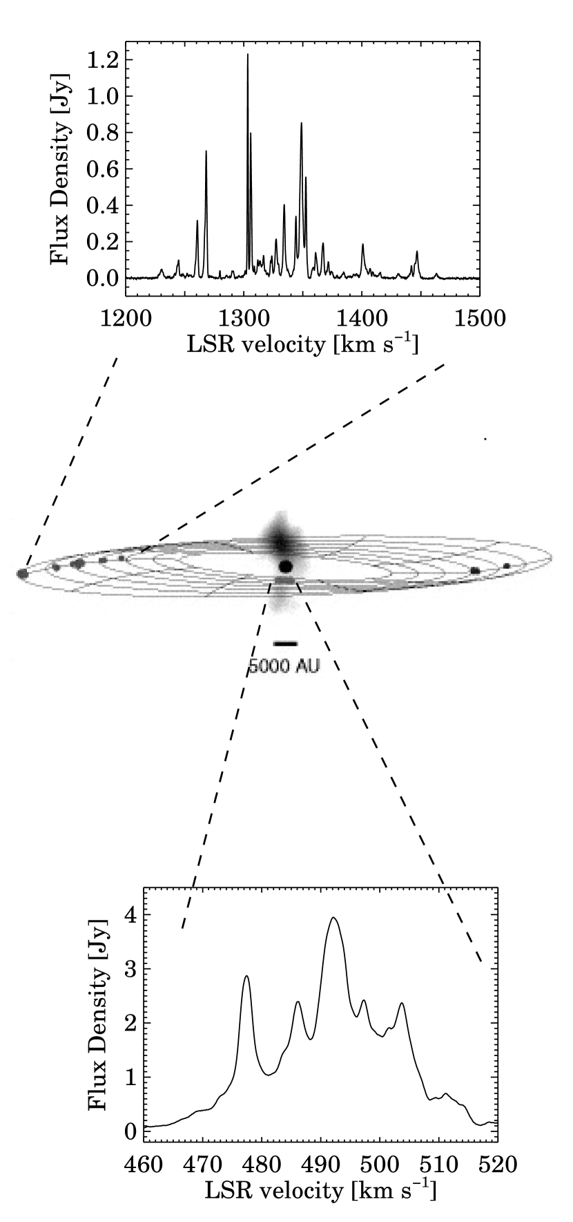
Figure 1.— Correspondence between maser features in velocity at 22.2 GHz and their location in the disk. Middle: The warped accretion disk, defined by the kinematics of the maser spots, is shown as a wire grid (adapted from Moran et al. 1999), while the black dot marks the dynamical center of the system (the position of the SMBH). The gray-scale elongation in the center shows the 22 GHz synchrotron continuum emission (Herrnstein et al., 1998a). Top, bottom: The GBT spectra were taken on 2003 October 23 (see § 3 for details).

The discovery of a nuclear megamaser in a survey by Claussen et al. (1984) in NGC 4258 and the subsequent radio single-dish and interferometry imaging studies (Greenhill et al. 1995; Miyoshi et al. 1995) have improved our knowledge of the nuclear region and its kinematics on sub-parsec radii. The spatial distribution and line-of-sight velocities of the masers delineate the molecular portion of a thin, Keplerian (better to 1%) accretion disk that is nearly edge-on (tipped down by $\sim 8$°) and slightly warped (Moran et al. 1995; Herrnstein et al. 1996). The maser lines fall into three groups: a dense cluster near the systemic velocity of the galaxy, which lies close to the line-of-sight to the black hole (hereafter referred to as “systemic maser lines”), bracketed by two groups of less densely packed lines offset by $\pm$ (800$-$1000) km s^-1. These high-velocity masers have very small accelerations compared with the systemic masers (Bragg et al., 2000) and are distributed over different radii close to a line perpendicular to the line of sight, the so-called “midline” (Fig. 1); hence their line-of-sight velocities are close to the Keplerian orbital velocities. The inner radius of the maser annulus is approximately 0.14 pc and its outer radius approximately 0.28 pc (for a distance of $D$ = 7.2 Mpc, Herrnstein et al. 1999; 1″ corresponds to 35 pc at that distance) from the central black hole with $M_{\rm{BH}}=(3.9\pm 0.4)\times 10^{7}M_{\sun}$ (Miyoshi et al., 1995). There is a prominent north-south twisted jet on kiloparsec scales observed in the radio, in H$\alpha$, and in X-rays (e.g., Cecil 2000; Wilson et al. 2001 and references therein). It appears to be an extension of the radio nuclear jet seen at sub-parsec distances from the dynamical center (Herrnstein et al., 1997) and to have an axis that is well aligned with the rotation axis of the maser accretion disk. We note that the angular momentum vectors are quite misaligned at kiloparsec and sub-parsec distances from the central engine: the edge-on accretion disk, as traced by the masers, makes an angle of $\sim 120\arcdeg$ to the galactic disk of the host galaxy, a SAB(s)bc spiral (Tully, 1988), i.e., the maser accretion disk is counter-rotating with respect to the larger galactic structure.

There have been estimates made of magnetic field strengths at kiloparsec radii in NGC 4258. Krause & Löhr (2004) obtained VLA 8.44 GHz ($\lambda$3.6 cm) continuum observations of the jets of NGC 4258 and detected linear polarization at a level of $35\%-65\%$ along the northern jets whose interpretation in the context of synchrotron emission mechanisms suggests the presence of an ordered magnetic field. Assuming energy equipartition between the magnetic field and the relativistic particles in the northern jet, and an electron-proton (electron-positron) composition, they obtained an average $B$ field of $\sim$310 $\mu$G ($\sim$90 $\mu$G). These values reflect the poloidal component of the global magnetic field at a distance of $\sim$ $1-4$ kpc along the jet.

By searching for Zeeman-induced circular polarization in the maser lines, the strength and direction of the magnetic field parallel to the line of sight across the maser emission region can be directly determined. The effort to scrutinize a well-isolated, 1.2$~{}{\rm km~{}s^{\scriptscriptstyle-1}}$ wide maser line in the redshifted group at 1306$~{}{\rm km~{}s^{\scriptscriptstyle-1}}$ by Herrnstein et al. (1998b) yielded no detection of polarization in the VLA data taken in 1995. The resulting limit to the circular polarization of 0.5% corresponds to an upper bound of approximately 300 mG for the toroidal component of the magnetic field. The Zeeman technique constitutes the most direct way of obtaining the magnitude and direction of the magnetic field. Magnetic field estimates have been derived from other techniques (e.g., Jones et al. 2000), but they are relatively indirect and model dependent, relying on assumptions of equipartition between thermal and magnetic energy, and adopted values of electron density and temperature at various radii. The initial attempt to measure polarization in NGC 4258 was made by Deguchi et al. (1995) who reported an upper limit on linear polarization of 20% for the high-velocity water maser components and of 15% on the systemic components.

The format of this paper is as follows: In § 2, we briefly outline the theoretical background for understanding the Zeeman effect in the water molecule, and describe the technical details of how to measure the Zeeman effect. We present and discuss two data sets in § 3 and report the measured upper limits on the magnetic field for the various maser lines in § 4. We discuss the interpretation of the Zeeman observations in § 5 and give conclusions with § 6.

2. THE ZEEMAN EFFECT IN WATER

The maser emission at 22.235 GHz involves the rotational energy states $J_{\rm{K+K-}}$ = 5₂₃ and $J_{\rm{K+K-}}$ = 6₁₆ of ortho-water, which lie $\sim$600 K above the ground state. This rotational transition consists of six hyperfine components, but it is generally believed that only the strongest three hyperfine components ($F=7-6,6-5,5-4$) contribute significantly to the maser emission (Deguchi & Watson 1986; Nedoluha & Watson 1991; Vlemmings et al. 2001, hereafter V01) with velocity separations of 0.45 and 0.58$~{}{\rm km~{}s^{\scriptscriptstyle-1}}$ between them (those separations are marginally within a typical maser line width of $\sim 0.8-$1$~{}{\rm km~{}s^{\scriptscriptstyle-1}}$).

In the presence of an external magnetic field, each hyperfine component splits into three groups of lines with characteristic polarization properties: the $\pi$ transitions ($\Delta M_{F}=0$) produce radiation linearly polarized along the external $B$ field, with negligible frequency displacements from the parent-hyperfine transition. The $\sigma^{\pm}$ transitions ($\Delta M_{F}=\pm 1$) generate emission whose $E$ field vector rotates in a circle in the plane perpendicular to the external $B$ field direction and are symmetrically offset from the parent-hyperfine in frequency by $\pm\Delta\nu_{Z}$ (we follow the notation used in V01; see their Fig. 1 showing the theoretical Zeeman pattern). Since the water molecule is non-paramagnetic, the splitting is very small ($\Delta\nu_{Z}\sim 1$ Hz mG^-1 or $10^{-5}$$~{}{\rm km~{}s^{\scriptscriptstyle-1}~{}mG^{\scriptscriptstyle-1}}$ compared to, e.g. up to 3 kHz mG^-1 or 0.6$~{}{\rm km~{}s^{\scriptscriptstyle-1}~{}mG^{\scriptscriptstyle-1}}$ for the OH molecule at 18 cm) and much less than the thermal line width of the maser features for expected sub-Gauss $B$ fields ($\Delta\nu_{Z}\sim 10^{-4}-10^{-3}\Delta\nu_{L}$). For a $B$ field along the line of sight, the $\sigma^{\pm}$ components appear in left-circular polarization (LCP) and right-circular polarization (RCP), respectively, and their slight frequency separation can be detected as an “S” shaped profile in the Stokes $V$ [= (LCP $-$ RCP)/2 ] spectrum for a simple Gaussian line profile (Fig. 2). This S profile is proportional to the derivative of the Stokes $I$ [=(LCP + RCP)/2 ] spectrum in the small splitting case (Fiebig & Güsten 1989, hereafter FG89; Herrnstein et al. 1998b; V01; see also Appendix A).

Figure 2.— Theoretical Stokes $V$ spectra for the three strongest hyperfine components $F=7-6,6-5$ and $5-4$, under the assumption of LTE at the predicted hyperfine rest velocities (centered at the hyperfine rest velocity of $F=6-5$). The $B$ field is 50 mG and the line width 0.8$~{}{\rm km~{}s^{\scriptscriptstyle-1}}$ (FWHM).

By modeling the theoretical H₂O Zeeman pattern and convolving it with Gaussian profiles of differing line widths, FG89 constructed a set of synthetic Stokes $V$ spectra and found the following relationship between the applied $B$ field and the resulting circular polarization:

$$\frac{V_{\rm{max}}}{I_{\rm{max}}}=\frac{A_{\rm{F-F^{\prime}}}B_{||}}{\Delta v_{L}},$$ (1)

where $V_{\rm{max}}$ is the maximum of the $S$ curve, $I_{\rm{max}}$ is the maximum in Stokes $I$, $B_{||}$ is the magnetic field parallel to the line-of-sight, $B_{||}=B\rm{cos}\theta$ (where $\theta$ is the angle between the $B$ direction and the line of sight), and $A_{\rm{F-F^{\prime}}}$ is a coefficient that depends on which hyperfine component is assumed. In the case where the hyperfine lines appear individually, $A_{7-6}$ = 0.0134$~{}{\rm km~{}s^{\scriptscriptstyle-1}~{}G^{\scriptscriptstyle-1}}$ for the $F=7-6$ hyperfine that possesses the largest transition probability; $A_{6-5}$ = 0.008$~{}{\rm km~{}s^{\scriptscriptstyle-1}~{}G^{\scriptscriptstyle-1}}$ for $F=6-5$ and $A_{5-4}$ = 0.001$~{}{\rm km~{}s^{\scriptscriptstyle-1}~{}G^{\scriptscriptstyle-1}}$ for $F=5-4$.

Equation (1) does not account for the non-thermal nature of maser emission, which includes inverted, non-thermal, population distributions and amplification of emission. Nedoluha & Watson 1992 (hereafter NW92), Watson & Wiebe 2001 and, more recently, Vlemmings et al. 2002 (hereafter V02), conducted a series of studies in which they solved the radiative transfer and rate equations numerically for water masers in a magnetic field, extending the pioneering analytic work of Goldreich, Keeley, & Kwan (1973). These numerical simulations account for saturation effects and the presence of the three strongest hyperfine components and their magnetic substates. Their major findings were that the “thermal” equation (1) is an excellent approximation for the case of maser polarization induced by a magnetic field with an effective coefficient $A_{\rm{F-F^{\prime}}}$ of 0.020$~{}{\rm km~{}s^{\scriptscriptstyle-1}~{}G^{\scriptscriptstyle-1}}$ (appropriate for the presence of the three strongest hyperfines). The estimate of the $B$ field via equation (1) is accurate to within a factor of 2, as long as the water maser is not highly saturated, i.e., has a linewidth $\lesssim$ 0.8 ${\rm km~{}s^{\scriptscriptstyle-1}}$(NW92). In those numerical simulations, maser propagation was modeled in one dimension. However, initial calculations in 2D by V02 suggest that the resulting Zeeman $S$ curves might be slightly narrower and have a distorted profile, than dedyced from 1D calculations. Gray (2003) did a study of maser polarization models in which he compared his general models to the ones put forth by Watson and collaborators (Watson, 1994; Nedoluha & Watson, 1994) and found that his equations can be reduced to the ones by Watson, for the limiting case of small Zeeman splitting.

In summary, we adopt $A_{\rm{F-F^{\prime}}}$ = 0.020 km s^-1 G^-1 for the $S$-curve model, where the Stokes $V$ profile is proportional to the derivative of Stokes $I$, appropriate for the presence of the three strongest water hyperfines in a masing environment. This Zeeman splitting coefficient is larger by a factor of 1.5 than for the LTE model where solely the hyperfine component with the largest transition probability under LTE is present. Following other Zeeman experiments in the radio regime (e.g., Goodman 1989, Heiles 2001), we adopt the IEEE convention for circular polarization, where a magnetic field pointing away from the observer is $positive$ and produces a LCP component at a $lower$ velocity than the RCP component.

Several water maser polarization experiments have been conducted and interpreted in the framework of equation (1), with line-of-sight magnetic fields inferred on the order of $10-50$ mG in Galactic star-forming regions (FG89; Sarma et al. 2001, 2002). These results agree with magnetic field strengths expected for a wide range of probed densities in molecular clouds, which are subject to flux freezing and ambipolar diffusion, thus providing corroborating evidence for the cogency of the Zeeman interpretation. Furthermore, line-of-sight magnetic fields have been inferred on the order of $50-3000$ mG in circumstellar envelopes of late-type stars (V02). These values are consistent with $B$ field estimates based on OH maser observations for a reasonable radial scaling of the $B$ field.

There are two types of maser lines in the spectrum of NGC 4258, which require slightly different treatments to measure the Zeeman effect. For the well-isolated redshifted and blueshifted high-velocity maser lines, the standard $S$-curve analysis method as outlined above works well. For the systemic features, which are heavily blended in velocity space, we developed a variant of the $S$-curve method. Our new technique is more appropriate since it does not require the a priori knowledge of the velocity components. In this procedure, we cross correlate the LCP and RCP spectra to determine the net velocity offset (see Appendix B for details). This cross correlation method (see also Heiles 1988 for a slightly different treatment in the case of observations of blended thermal H I features) is based on the assumption that the $B$ field strength and direction remain constant over the emission region, i.e., that the Zeeman-induced velocity shift is constant across the spectrum.

From simple statistical arguments, supported by Monte Carlo simulations (Appendix B.2), the rms sensitivity to the LOS $B$ field ($\sigma_{B_{||}}$) is given by the following relationship (which applies for both the $S$-curve and the cross correlation method),

$$\sigma_{B_{||}}=\frac{1}{2}\frac{\Delta v_{L}}{A_{\rm{F-F^{\prime}}}~{}SNR}\frac{1}{\sqrt{N}}~{}~{},$$ (2)

where $\Delta v_{L}$ is the FWHM line width, $A_{\rm{F-F^{\prime}}}$ the Zeeman splitting coefficient, $SNR$ the signal-to-noise ratio for the specific line (in Stokes $I$) and $N$ the number of lines over which the fit is performed. This result is appropriate if the $N$ lines are not heavily blended. For differing line strengths and line widths of the spectrally blended lines, as found in the cross correlation technique, the $\Delta v_{L}/(SNR~{}\sqrt{N})$ factor must be replaced by an appropriate average.

3. OBSERVATIONS AND DATA REDUCTION

3.1. VLA Data

Data were taken on 2001, December 16 in spectral line and full polarization mode with the Very Large Array (VLA) of the National Radio Astronomy Observatory (NRAO) in its D configuration for approximately 12 hours at K Band (22.2 GHz). The resulting synthesized half-power beamwidth is 2.8 arcsec. In this beam, the maser spots (with intrinsic sizes of less than 100 $\mu$arcsec and inter-maser-separations of several milliarcsec as shown by VLBI observations; Miyoshi et al. 1995; Moran et al. 1995) appear as one point source and are not resolved; therefore, beam effects such as beam squint and beam squash do not affect our data. The segregation among the various maser spots occurs in velocity space, since the maser spots possess different orbital velocities. The observations of an isolated high-velocity feature at 1269 km s^-1 had to be interlaced with those of the systemic features due to the limited bandwidth of the VLA. The calibrators were observed separately for the two different frequency bands. The observations were performed with a bandwidth of 1.56 MHz with 128 channels, yielding a channel spacing of 12.2 kHz (or 0.16 $~{}{\rm km~{}s^{\scriptscriptstyle-1}}$). With uniform weighting the spectral resolution is 0.19$~{}{\rm km~{}s^{\scriptscriptstyle-1}}$, which corresponds to $\sim 1/5$ of the high-velocity maser line width. The first three hours of the observations experienced snow fall, with skies gradually clearing thereafter.

Figure 3.— GBT total power data with a bandwidth of 200 MHz. Note the flat baseline after removing a running mean that excluded the line-displaying regions. Inserts show zooms on the red- and blue-shifted high-velocity lines, respectively. The rms noise in each channel is 2.9 mJy. The feature at 1647$~{}{\rm km~{}s^{\scriptscriptstyle-1}}$ is a highly significant new discovery. It is the most redshifted high-velocity feature discovered in NGC 4258, and it extends the inner boundary of the maser disk to 0.12 pc, based on the Keplerian rotation curve.

The data were edited, reduced, and calibrated with standard spectral line techniques in AIPS, including bandpass, amplitude and phase calibration. Amplitude calibration was performed with respect to 3C 147, a VLA calibrator with known flux density at 22 GHz, phase calibrations relative to 1146+399, and bandpass calibrations using observations of 0854-201. The system temperatures of the K-band receivers in nine of the antennas were in the range of $100-130$ K, whereas the new K-band receivers, residing in 17 out of the 26 operational antennas at the date of observations, had system temperatures of $60-80$ K. The amplitude calibration is estimated to be accurate to within 15%. Strong internal radio-frequency-interference was present in the calibrator data taken with the old receivers at the frequency corresponding to that of the systemic maser emission and had to be removed from the data set.

We performed linear polarization calibration in two steps: first we used the observations of the strong source 0854+201 over a range of parallactic angles to correct for the imperfect feed responses (as expressed by the so-called “leakage terms”, which are on the order of a few % for the VLA K band feeds). Secondly, we determined the phase offset between LCP and RCP by observing 3C286, a polarized source with a known and invariant polarization angle. For circular polarization calibration, an additional step involved correcting for the differences in gain for LCP and RCP and was performed during the analysis of the polarization data (see § 4).

Table 1Journal of H₂O Maser Observations

Parameter	VLA Data		GBT Data
	Set I	Set II
Date	2001 Dec 16	2001 Dec 16	2003 Oct 23
Radio LSR center velocity [${\rm km~{}s^{\scriptscriptstyle-1}}$]	495	1268	550
Total Bandwidth [${\rm km~{}s^{\scriptscriptstyle-1}}$]	21	21	2700
Channel spacing [${\rm km~{}s^{\scriptscriptstyle-1}}$]	0.16	0.16	0.16
Integration time [min]	241	231	348
1 $\sigma$ noise in Stokes $I$ [mJy]	2.4	2.4	2.9

3.2. GBT Data

We took spectral line data in RCP and LCP on 2003 October 23 with the Robert C. Byrd Green Bank Telescope (GBT) of the NRAO. With an off-axis feed arm, the GBT delivered an unblocked aperture and low sidelobes with a FWHM beamwidth of 33″ at 22.2 GHz. The spectrometer had a bandwidth of 200 MHz configured to provide a channel spacing of 0.164$~{}{\rm km~{}s^{\scriptscriptstyle-1}}$ with its 16384 channels over 200 MHz (2700 ${\rm km~{}s^{\scriptscriptstyle-1}}$). The K-band receiver for the upper frequency range (22$-$26.5 GHz) had two beams, each beam producing two polarization channels. The data were taken in beam-switched mode with beam throws of the order of 4′, the angular distance between the pair of beams. The cycle time of two minutes was sufficient to compensate for atmospheric fluctuations. In this fashion, one beam of the telescope was always pointing at the source. A total of eight hours of data were taken, including pointing and focusing observations after every hour of source observation. Applying the local pointing corrections improved the pointing uncertainty to $\lesssim$ 2$\arcsec$. The effective on-source time was 348 minutes and the zenith opacity $\sim$0.07.

The gain curve, which describes the efficiency of the antenna as a function of elevation, had been determined from observations of the radio source NGC 7027 over a range of elevations. The gain curve with the active surface-control enabled indicates a peak antenna efficiency of $\eta$ = 0.6 at an elevation of $\sim 30\arcdeg$ and stays comparatively flat ($\eta\approx 0.5-0.6$) over a wide range of elevations ($20\arcdeg-80\arcdeg$). The rms deviation of the gain measurements around the best-fit polynomial model, which is applied to the data for gain correction, was about 10%. Amplitude calibration was performed via injection of a signal from a noise diode every 0.25 sec. Data reduction was performed with a customized IDL procedure.

The residual baseline variations in the spectra were eliminated by subtracting a running mean computed over intervals of 256 channels (41$~{}{\rm km~{}s^{\scriptscriptstyle-1}}$) that excluded the line-bearing regions; this procedure yielded flat baselines in the final spectrum (Fig. 3). The system temperatures for the GBT data ranged from $35-50$ K and quoted flux densities are accurate to 10%. The largest source of uncertainty is the inaccurate knowledge of the strength of the noise diodes over the large bandwidth of the GBT data. We note that the uncertainty in the absolute intensity scale has little impact onto the reported results of the magnetic field upper limits: only a differential measurement, the SNR, determines the upper limit (eq. [2]).

Table 1 lists a summary of the specifications of both data sets. The velocities in this paper follow the radio definition of Doppler shift ($\Delta\nu/\nu=-v/c$) and are computed with respect to the local standard of rest (LSR).

4. RESULTS AND INTERPRETATION

Figure 4.— VLA data of the high-velocity feature at 1269 ${\rm km~{}s^{\scriptscriptstyle-1}}$ with Zeeman analysis. Top: Stokes $I[=(\rm{LCP}+\rm{RCP})/2]$ spectrum. Middle: The Stokes $V[=(\rm{LCP}-\rm{RCP})/2]$ spectrum, which is adjusted by having removed a scaled replica of the total power profile, determined by the $c_{2}$ parameter in equation (3) for this fit. Superimposed are the Zeeman $S$ curves for the upper limit of $\pm 90$ mG on the LOS magnetic field as reported in Table 2. Bottom: Total linear polarization spectrum [Stokes $(Q^{2}+U^{2})^{1/2}$].

Figure 5.— Similar to Figure 4, but for the strongest redshifted high-velocity feature in the GBT spectrum, except no linear polarization data could be obtained with the GBT spectrometer. The 1-$\sigma$ $S$ curves for $B^{\rm{lim}}_{||}=\pm$90 mG is overplotted.

For circular polarization data, instrumental gain differences between LCP and RCP cause a portion of the Stokes $I$ profile to appear in the Stokes $V$ spectrum. This effect is mitigated by simultaneously fitting a replica of Stokes $I$ to the Stokes $V$ spectrum in addition to a scaled derivative of Stokes $I$ in the least-squares sense (e.g., Troland & Heiles 1982; Sault et al. 1990) :

$$V(v)=c_{1}~{}\frac{dI(v)}{dv}+c_{2}~{}I(v).$$ (3)

Here, $c_{2}$ denotes the instrumental polarization term. The factor $c_{1}$ is a measure of the Zeeman splitting and corresponds to $A_{\rm{F-F^{\prime}}}B\rm{cos}\theta/\sqrt{2}$ (Appendix A). This calibration procedure is equivalent to the assumption that equal flux should be present in both the LCP and RCP spectra, i.e., that the circular polarization spectra are intrinsically anti-symmetric. However, theoretical maser polarization simulations (see § 2) produce $V$ spectra that are asymmetric due to the presence of hyperfine structure. Efforts to verify the intrinsic shape of the $V$ spectrum observationally are hampered by the the fact that it has been impossible to determine the instrumental circular polarization independently well enough to the requisite degree of $P_{V}=V/I\sim 0.1\%$ (Zhao, Goss, & Diamond, 1993). In order for the derived magnetic fields strength $B_{||}$ to be counted as a detection, we require the field strength to be greater than 3 times the associated uncertainty, $\sigma_{B_{||}}$. With this criterion, we did not make any Zeeman-induced circular polarization detection.

4.1. High-velocity Features

Figure 4 shows the Stokes $I[=(\rm{LCP}+\rm{RCP})/2]$, i.e., total power, VLA spectrum of the redshifted high-velocity feature at 1269 km s^-1 with a thermal rms noise of about 2.4 mJy (in a 0.16$~{}{\rm km~{}s^{\scriptscriptstyle-1}}$ resolution interval; see Table 1). The high-velocity line was best fit by a two-component Gaussian, such that the main line is centered at 1268.6$~{}{\rm km~{}s^{\scriptscriptstyle-1}}$and has a FWHM line width of $\Delta v_{L}$ = 1.01$~{}{\rm km~{}s^{\scriptscriptstyle-1}}$. A formal minimum $\chi^{2}$ fit of the Stokes $V[=(\rm{LCP}-\rm{RCP})/2]$ spectrum to equation (3) indicated a 1-$\sigma$ upper limit to any intrinsic circular polarization of $P_{V}\lesssim 0.08$% in the 1269 km s^-1 feature. For a maser Zeeman splitting coefficient of $A_{\rm{F-F^{\prime}}}=0.020$$~{}{\rm Hz~{}mG^{\scriptscriptstyle-1}}$, $\sigma_{B_{||}}\approx$ 40 mG (1 $\sigma$). This value is the same, as expected, as the value derived from equation (2) and Monte Carlo Simulations (Appendix B.2). From a conservative estimate for the upper limit on the magnetic field along the line-of-sight, $\mid B^{\rm{lim}}_{||}\mid=\mid B^{\rm{output}}_{||}\mid+\sigma_{B_{||}}+\sigma_{\sigma_{B_{||}}}$, we obtained $B_{||}\lesssim$ 90 mG (Table 2), where $\sigma_{\sigma_{B_{||}}}$ stands for the uncertainty in $\sigma_{B_{||}}$ and is estimated from Monte Carlo simulations (§ B.2). This feature is located at a radial distance of 0.27 pc from the SMBH (70,000 in units of Schwarzschild radii, $R_{S}=2GM_{\rm{BH}}/c^{2}$, for $M_{\rm{BH}}=3.9\times 10^{7}M_{\sun}$). Following convention, the middle panel of Figure 4 shows the Stokes $V$ spectrum intrinsic to the source, i.e., after removing a residual replica of Stokes $I$. Superimposed are the 1-$\sigma$ Zeeman $S$ curves for B${}_{||}^{\rm{lim}}=\pm$90 mG. The bottom panel of Figure  4 shows the total linear polarization [Stokes $(Q^{2}+U^{2})^{1/2}$] spectrum: no fractional linear polarization [Stokes $(Q^{2}+U^{2})^{1/2}/I$] at a level of 0.1% (1 $\sigma$) is detected.

For the GBT dataset, the combination of low system temperatures and a new spectrometer with a large bandwidth promised higher sensitivity for Zeeman detection. However, the variable nature of masers caused a decrease in the SNR during our observations and no Zeeman-induced circular polarization could be detected in any of the numerous features. The $S$-curve analysis yielded an upper limit for the strongest high-velocity feature at 1303.3$~{}{\rm km~{}s^{\scriptscriptstyle-1}}$ of B${}_{||}\lesssim$90 mG, similar to the VLA experiment (Table 2). Figure 5 shows the Stokes $I$ spectrum (top) with a thermal rms noise of 2.9 mJy (in a 0.16$~{}{\rm km~{}s^{\scriptscriptstyle-1}}$ resolution interval). This feature is best-fit by a one-component Gaussian model of width 0.79$~{}{\rm km~{}s^{\scriptscriptstyle-1}}$ (FWHM), centered at 1303.3$~{}{\rm km~{}s^{\scriptscriptstyle-1}}$. The instrumentation-corrected Stokes $V$ spectrum is displayed in the bottom panel of Figure 5 with the overlayed 1-$\sigma$ $S$ curves for B${}_{||}^{\rm{lim}}=\pm 90~{}\mathrm{mG}$. This feature is located at a distance of 0.25 pc from the central black hole, which corresponds to 62,000 $R_{S}$. Linear polarization data could not be obtained with the GBT spectrometer at the time of observations.

In this case, B_|| corresponds to the toroidal magnetic field and our limits are significant on the assumption that B_|| is not tangled over the maser emission region of $\lesssim$ 0.003 pc (or $\lesssim 10^{16}$ cm) (Moran et al., 1995). If the 22.2 GHz water vapor line consists solely of the $F=7-6$ hyperfine component, the $B$ field estimates have to be multiplied by a factor of 1.5. This result is an improvement of the upper limit of B${}_{||}\lesssim$ 300 mG derived by Herrnstein et al. (1998b) on a feature at 1306 km s^-1 using a similar method.

Hydro dynamic and MHD turbulence are expected in accretion disks. Assuming a Kolmogorov power spectrum for turbulent magnetic fields in a circumnuclear disk, Watson & Wiebe (2001) produced realistic simulations of total-power water maser spectra and found that the consequences for circular polarization were not serious. In the case of turbulent fields, they suggested that equation (1) underestimates the magnitude of the magnetic field generally by a factor of about 3. In their calculations, they assumed that the turbulence length for the radial scale is the same as the scale height of the disk, $H$, as they assumed isotropic turbulence where the longest wavelength is set by the height. However, C. Gammie (2004, private communication) estimated that most of the power may be contained on scales of the order 40$H$. Since the length of the masers and $H/R$ are estimated to be $\lesssim$0.003 pc and $\lesssim$0.0025, respectively (Moran et al., 1995), the turbulence length according to Gammie is larger than the maser length, by a factor of 4$-$10. For turbulence lengths that are considerably larger than the maser amplification length, few magnetic field reversals are expected across the maser length. Thus in summary, we conclude that it is unlikely that the non-detection of Zeeman-induced circular polarization is due to a scenario where turbulent magnetic fields quench the maser polarization signal due to magnetic field reversals.

4.2. Systemic Features

Figure 6.— Top: VLA total power [Stokes $I$ = (RCP+LCP)/2] data of the systemic features. Middle: Renormalized circular polarization spectrum [Stokes $V$ = (RCP$-$LCP)/2]. Bottom: Linear polarization data [Stokes $(Q^{2}+U^{2})^{1/2}$].

Table 2H₂O Maser Parameters and Zeeman Interpretation

Data Set	Line center	FWHM	Io	Fitted Range	B||	$\sigma_{B_{||}}$	$\sigma_{\sigma_{B_{||}}}$	B${}^{\rm{lim}}_{||}$ (1$\sigma$)	R
	[${\rm km~{}s^{\scriptscriptstyle-1}}$]	[${\rm km~{}s^{\scriptscriptstyle-1}}$]	[mJy]	[${\rm km~{}s^{\scriptscriptstyle-1}}$]	[mG]	[mG]	[mG]	[mG]	[pc]
VLA	1268.6	1.01	1795	1266.5$-$1270.0	-47	38	5	90	0.27
GBT	1303.3	0.79	1212	1302.0$-$1304.5	40	44	6	90	0.25
VLA	499.1	…	4553	486.0$-$504.0	29	16	4	49	0.14
GBT	492.3	…	4102	472.0$-$507.0	7	19	4	30	0.14

For the cross correlation method, we performed an equivalent gain calibration procedure by requiring the integrated line fluxes of LCP and RCP to be equal. Simulations and application of both calibration methods to the well-isolated features yield the same $B$ field estimates and uncertainties. The systemic maser lines are stronger and more numerous, thereby improving the sensitivity to the $B$ field, but have broader line widths than the high-velocity features and are heavily overlapped, decreasing the sensitivity.

Figure 7.— Top: GBT total power [Stokes $I$ = (RCP+LCP)/2] data of the systemic features. Bottom: Renormalized circular polarization spectrum [Stokes $V$ = (RCP$-$LCP)/2].

For the VLA data, we performed the cross correlation technique on those systemic maser lines that occupy the inner 90% of the bandwidth, in order to avoid passband problems at the edges of the spectrum. We derived a value of $B_{||}=29\pm 16$ mG (Fig. 6). Though this result is formally a 2 $\sigma$ detection, we do not count it as a significant detection (defined as a detection with a significance level of 3 $\sigma$), but rather report an upper limit of B${}_{||}\lesssim$ 50 mG (see Table 2 for computation). There are deviations near 493$~{}{\rm km~{}s^{\scriptscriptstyle-1}}$ and at 499$~{}{\rm km~{}s^{\scriptscriptstyle-1}}$ in the Stokes $V$ spectrum, which are responsible for the 2$\sigma$ result. There is no clear detection of fractional linear polarization at a level of 0.3% (1 $\sigma$) (Fig. 6, bottom panel). However, the conditions in the masing medium could give rise to internal Faraday rotation along the maser amplification path, leading to depolarization of a strong linearly polarized signal (see, e.g., §13.6 of Thompson, Moran, & Swenson 2001). The requisite electron density for complete depolarization by this mechanism (i.e. differential Faraday rotation of $\pi$) is $n_{e}\approx\pi\left(8.1\times 10^{5}\lambda^{2}B_{||}L\right)^{-1}$, where $\lambda$ is the observing frequency in meters, $B_{||}$ the $B$ field along the line-of-sight in Gauss, $L$ the pathlength over which depolarization is taking place in pc, and $n_{e}$ is the electron density in cm^-3. For $\lambda$ = 1.35 cm, $L$ = 0.003 pc (Moran et al., 1995), $B_{||}\lesssim 0.03$ G, one obtains $n_{e}\sim$200 cm^-3. For an assumed average molecular density of $10^{9}$$~{}{\rm cm^{\scriptscriptstyle-3}}$, this corresponds to an ionization fraction of $x_{e}\sim$ 10^-7. These low values are well within the range of the expected ionization fraction. Models by Neufeld, Maloney, & Conger (1994) and Neufeld & Maloney (1995), in which oblique X-ray illumination is heating the gas in the molecular accretion disk of NGC 4258 and other megamaser galaxies, give a theoretical upper limit of $x_{e}\sim 10^{-5}$. Note that there are observations of strong linear polarization (up to 65%) in galactic water masers (Garay, Moran, & Haschick, 1989), which arise in star formation regions.

Cross correlating the GBT spectra of the systemic features in LCP and RCP leads to a 1-$\sigma$ upper limit of B${}_{||}\lesssim$30 mG (Fig. 7 and Table 2). We chose the velocity range of the systemic maser lines such as to maximize the number of included features, while minimizing the extent of the baseline modulation seen in the renormalized Stokes $V$ spectrum (bottom panel of Fig. 7). Note that the different appearance of the systemic features in the two datasets are due to both time variability and centripetal acceleration of $\sim$10 ${\rm km~{}s^{\scriptscriptstyle-1}}$yr^-1 (Bragg et al., 2000).

In the case of the systemic features, $B_{||}$ refers to the ordered radial component of the $B$ field, assuming the features are threaded by a $B$ field constant in magnitude and direction. They are located at a distance of $R\approx 0.14$ pc ($37,000~{}R_{S}$) from the central black hole (Bragg et al., 2000, as derived from the observed acceleration of the systemic features). The features are distributed over an azimuthal angle in the disk of about 8$\arcdeg$, or about 0.02 pc. Recently, Herrnstein et al. (2005) estimate that the systemic features are located in a bowl-shaped depression of the warped disk and occupy a region of length 0.05 pc along the LOS.

Table 2 lists the details and summary of the individual Zeeman fits and their interpretation.

4.3. Saturation Effects

Some theoretical investigations have shown that the degree of observed circular water maser polarization depends also on the saturation state of the masers. Masers begin to saturate when $R/\Gamma\gtrsim 1$, and reach full saturation when $R/\Gamma\gtrsim 100$, where $R$ is the rate of stimulated emission and $\Gamma$ the decay rate, with $\Gamma$ = 1 s^-1 from the lifetime of involved IR transitions.

The stimulated emission rate of a maser is given by $R=A~{}S_{\nu}~{}c^{2}/(8~{}\pi~{}h\nu^{3})\times(\Omega_{b}/\Omega_{s})$ (Reid & Moran, 1988), where $A$ is the Einstein coefficient for spontaneous emission ($2\times 10^{-9}$ s^-1 for the water transition), $S_{\nu}$ the specific flux density of the maser, and $\Omega_{b}$ and $\Omega_{s}$ are the beaming and subtended solid angle of the maser. For a cylindrical maser model, $\Omega_{b}=(d/L)^{2}$, and $\Omega_{s}=(d/D)^{2}$, where $d$ is the cross section diameter of the maser, $L$ is the maser length, $D$ is the distance to the maser source. Hence, we can write for $D$ = 7.2 Mpc,

$$R=50\left(\frac{S_{\nu}}{1~{}\rm{Jy}}\right)\left(\frac{L}{10^{16}~{}\rm{cm}}\right)^{-2}\rm{s^{-1}}.$$ (4)

If the coherent velocity interval is 1 ${\rm km~{}s^{\scriptscriptstyle-1}}$, then the maximum coherent amplification length due to the line-of-sight gradient for a high-velocity maser feature at a radius of 0.2 pc is $0.2~{}\mathrm{pc}\times\sqrt{2~{}\mathrm{km~{}s^{-1}}/v_{\rm{rot}}}$ or $3\times 10^{16}$ cm. Hence, $R_{\rm{max}}$ is 5 s^-1 for the high-velocity masers with typical flux densities $S_{\nu}=1~{}\mathrm{Jy}$. For the systemic masers, the beaming angle is known because of the clear velocity range of the systemic masers. It is 8°, so that $\Omega_{b}=0.015~{}\mathrm{sr}$. In this case, we can write $R=0.8~{}S_{\nu}~{}(d/10^{16}\mathrm{cm})^{-2}$. The maser spectrum is very crowded with the spacing between features of about 1$~{}{\rm km~{}s^{\scriptscriptstyle-1}}$ or larger. This means that $d\gtrsim 6\times 10^{14}$ cm, and $R$ is less than 500 for the systemic features with typical flux densities $S_{\nu}=2~{}\mathrm{Jy}$.

This means that the high-velocity masers are probably not saturated. Furthermore, the linewidth of 1.01$~{}{\rm km~{}s^{\scriptscriptstyle-1}}$ (FWHM) of the high-velocity feature at 1269$~{}{\rm km~{}s^{\scriptscriptstyle-1}}$ is inconsistent with a rebroadened, highly saturated maser that is a blend of the 3 strongest hyperfine components, for the spectral line breadth at high saturation is expected to be FWHM = 1.5 ${\rm km~{}s^{\scriptscriptstyle-1}}$(NW92, Emmering & Watson 1994; Watson & Wyld 2003). In addition, Watson & Wyld (2000) favor $R/\Gamma\lesssim 1$ from numerical simulations of masers in a Keplerian disk with velocity gradients. The systemic features are probably slightly saturated, and might reach full saturation.

Even if the masers are fully saturated, the upper limit on the magnetic field would be lower by a factor of maximally 4 (V02 Fig. 7; NW92 Fig. 7) – consequently, at any event, our reported magnetic field upper limits are truly upper limits. Since saturation increases the observed circular polarization, even in the event of strong saturation, the true magnetic field is smaller than the quoted upper limit.

5. DISCUSSION

5.1. The Total Magnetic Field

We obtained upper limits on the toroidal and on the radial component of the magnetic field in the accretion disk of NGC 4258 by searching for Zeeman-induced circular polarization. Based on these results we did simulations to estimate the limit on the total magnetic field. Since the toroidal and the radial component, $B_{\rm{tor}}$ and $B_{\rm{rad}}$, were probed at only slightly different radii, but different locations in the disk, we regard them as representative values for the disk and thus assume they can be used to characterize the magnetic field at a specific point, i.e., radius.

Figure 8.— Result of simulations of the value of the total magnetic field ($B_{\rm{tot}}$) given our measured upper limits on the two components of the $B$ field. The percentage of simulations where the total $B$ field satisfies the upper limits on the toroidal and radial component and is therefore undetected with a sensitivity comparable to our measurements is plotted as a function of $B_{\rm{tot}}$. The dashed line indicates the 50% limit, i.e., in 50% of the trial runs the observational limits were met (see text for details).

We conducted a simulation by assigning random orientations to a range of total $B$ field strengths, $B_{\rm{tot}}=0-1000$ mG. For each value of $B_{\rm{tot}}$, 5000 random orientations were drawn, with uniform distributions in $B_{\rm{tor}}$, $B_{\rm{rad}}$, and $B_{\rm{pol}}$, the poloidal component.

For each orientation, the value of the two components of interest were compared to our observational upper limits. Figure 8 presents the results of the simulations: it shows the percentage of trials in which the toroidal and radial components of the intrinsic total $B$ field could not be detected with our observational accuracy as a function of the intrinsic total $B$ field. We find that the simulated orientations for the $B$ field would exceed measurements 50% of the time for a B_tot value of 130 mG. Thus, we adopt the estimate of 130 mG as the upper limit on the total $B$ field at a distance of 0.14 pc from the central SMBH. The Alfvén speed, $v_{A}=B/\sqrt{4\pi\rho}$, would be 2$-$20 ${\rm km~{}s^{\scriptscriptstyle-1}}$ for the the allowable range of densities of molecular hydrogen, $10^{8}-10^{10}$ $~{}{\rm cm^{\scriptscriptstyle-3}}$, and for $B_{\rm{tot}}\lesssim 130$ mG.

From simple hydrostatic equilibrium arguments where the magnetic pressure confines the masing gas, one could expect the following values for the $B$ field: From $B=\sqrt{8\pi n_{\rm{H_{2}}}kT_{k}}$, the minimum value would be $B_{\rm{min}}=10$ mG (for the minimum temperature of $T_{k}$ = 250 K and minimum molecular number density of $n_{\rm{H_{2}}}=10^{8}$ $~{}{\rm cm^{\scriptscriptstyle-3}}$) and the maximum value $B_{\rm{max}}=190$ mG (for $T_{k}=1000$ K and $n_{\rm{H_{2}}}=10^{10}$ $~{}{\rm cm^{\scriptscriptstyle-3}}$). LOS magnetic field measurements in starforming regions via water maser polarization observations lie within this range (FG89, Sarma et al. 2001, 2002), and polarization observations in envelopes of late-type starts indicate super-thermal magnetic fields of up to $\sim 0.1-3$ G (; ).

An alternate way of estimating the total magnetic field is by considering predictions from simulations of magnetic fields in accretion disk. A series of magnetohydrodynamic (MHD) simulations show that the combined presence of magnetic field and outwardly decreasing differential rotation can rapidly create MHD turbulence via the magneto-rotational instability (MRI) (Balbus & Hawley 1991; Stone et al. 1996; see also Balbus & Hawley 1998; Balbus 2003). This results in a greatly enhanced effective viscosity, which readily generates outward flow of angular momentum. Hawley, Gammie, & Balbus (1996) performed local three-dimensional simulations of magnetized shearing box models, with an weak ($p_{\rm{magnetic}}\ll p_{\rm{thermal}}$) and zero-mean magnetic field as part of the initial conditions. Using a variety of initial field strengths and geometries, they found that the large scale magnetic field is dominated by the toroidal component: $B_{\rm{tor}}^{2}:B_{\rm{rad}}^{2}:B_{\rm{pol}}^{2}\approx 10:5:1$. If MHD turbulence is dominant, one might expect a magnetic field configuration as found by Hawley et al. (1996). Hence, our measured upper limit on the radial component of the magnetic field then dictates an upper limit on the toroidal component of $\lesssim\sqrt{2}~{}30~{}\rm{mG}=43$ mG (GBT data), which is consistent with, and tighter than, the observationally determined upper limit of $B_{\rm{tor}}\lesssim 90$ mG at a slightly larger distance (Table 2). The MHD predicted total magnetic field would thus be $B_{\rm{tot}}=\sqrt{16/5}~{}B_{\rm{rad}}\lesssim$ 50 mG at a radius of 0.14 pc, where we used the limit from the GBT data on the radial component, and $B_{\rm{tot}}=\sqrt{16/10}~{}B_{\rm{tor}}\lesssim$ 110 mG at a radius of 0.2 pc, where we used the limit on the toroidal component. Since the radial limit is estimated closer to the black hole, we adopt $B_{\rm{tot}}\lesssim$ 50 mG as the MHD predicted total magnetic field.

There might be concerns that the magnetic field is not sufficiently coupled to the gas, as the ionization fraction prevalent in the molecular masing gas is probably very low. To probe this question, Menou & Quataert (2001) conducted studies on ionization, MHD and gravitational instabilities in AGN accretion disks and found that the conditions in NGC 4258’s accretion disk still satisfy the requirements for large Reynolds numbers; hence, the neutral particles are expected to be well-coupled to the magnetic field by collisions with the ions, and the MHD turbulence due to MRI in NGC 4258’s accretion disk is expected to be similar to that in an ionized plasma. They also found that the thermal ionization instability is unlikely to be a source of efficient angular momentum transport and, thus, does not induce large-amplitude luminosity fluctuations in the disk.

5.2. Effects of the Magnetic Field

Rees (1987); Bottorff et al. (1997), and more recently, Bottorff & Ferland (2000), have argued that magnetic fields of strength $\sim 5-10$ G confine the clouds that populate the broad-line regions (BLRs) in AGNs at distances $R\sim 10^{17}-10^{18}$ cm from the SMBH. Ho et al. (1997) report the detection of a broad H$\alpha$ component in high-resolution, high S/N total-light spectra of NGC 4258 (after decomposing the emission lines), with a FWHM of 1700 ${\rm km~{}s^{\scriptscriptstyle-1}}$. We note that the detected emission lines in polarized light (i.e., light scattered off material surrounding the central source) probably emanate from the narrow-line region, not the BLR (Wilkes et al., 1995; Barth et al., 1999). From the virial estimate, $R_{\rm{BLR}}$, the position of the BLR, is approximately $M_{\rm{BH}}G/v^{2}$, with $v=fv_{\rm{FWHM}}$, where the factor $f$ depends on the details of the geometry, kinematics, and orientation of the BLR and is $\sqrt{3}/2$ for an isotropic distribution with random inclinations (Netzer, 1990). Thus, $R_{\rm{BLR}}\sim 2.4\times 10^{17}$ cm or 0.08 pc. This is smaller by a factor of $2-3$ than the distance regime the magnetic field upper limits reported here are probing. In order to confine the BLRs at that distance, the $B$ field strength would have to scale as $r^{-4}$ to reach the required high field strengths — since this scaling is unphysical, we conclude that magnetic pressure is unlikely to be the dominant force to confine a BLR of radius 0.08 pc in NGC 4258 (see, however, Laor 2003 for arguments on why NGC 4258 might not harbor BLRs). However, since this system is an obscured AGN, the width of the broad H$\alpha$ component could be larger, meaning the BLRs could be located closer to the SMBH and thus high magnetic fields could be reached at those distances. We note that our upper limits reflect $B$ fields in very dense masing gas and that the postulated $B$ fields responsible for confining the BLR clouds would be presumably lower as they pervade a more rarefied intercloud medium (be it relativistic or accretion-driven wind or accretion flow; Rees 1987).

Large scale poloidal fields may play an important role in collimating AGN jets (see, e.g. Begelman, Blandford, & Rees 1984). VLBI observations of M87, which contains one of nearest large-scale jets, show that the jet is well-collimated at $30-100$ Schwarzschild radii, and are interpreted as suggesting an accretion disk threaded by a strong poloidal magnetic field as the launching mechanism (Junor, Biretta, & Livio, 1999). The poloidal $B$ field component in NGC 4258’s accretion disk, which is observationally inaccessible, can be estimated to be $B_{\rm{pol}}\sim B_{\rm{rad}}/\sqrt{5}\lesssim$ 14 mG (GBT data) at a radius 0.14 pc (or 37,000 $R_{S}$) from MHD model constraints. Since for a steady-state thin accretion disk, which is in thermal equilibrium, the surface density goes as $r^{-3/4}$ (Frank, King, & Raine, 2002), the upper limit on $B_{\rm{pol}}$ at $r$ = 0.14 pc translates to $B_{\rm{pol}}\lesssim~{}$7 G at 10 $R_{S}$, for an $\alpha$-thin disk that extends inwards to $\sim$10 $R_{S}$. This is much less than the magnetic fields of strength $10^{2}-10^{4}$ G required for collimating radio jets (Blandford & Payne, 1982).

5.3. Mass Accretion Rate

Relating the thermal pressure at the midplane of the accretion disk to the magnetic pressure, the mass accretion rate can be estimated from the magnetic field strength. The thermal pressure on the midline is given by (e.g., Neufeld & Maloney 1995; Herrnstein et al. 1998b):

$$P_{\rm{th}}=\rho c_{s}^{2}=\frac{1}{3\pi\sqrt{2\pi}}\frac{GM\dot{M}}{c_{s}r^{3}\alpha},$$ (5)

where $\alpha$ is the Shakura-Sunyaev viscosity parameter, and $M$ the mass of the black hole.

Setting equation (5) equal to $\beta B^{2}/8\pi$, where the parameter $\beta$ is the ratio between the gas and the magnetic pressure $\beta=8\pi\rho c_{s}^{2}/B^{2}$ and is 1 for equipartition (note that $\beta$ is sometimes defined as $\beta=P_{\rm{tot}}/P_{\rm{mag}}$), we obtain

$$\dot{M}=\frac{3\sqrt{2\pi}}{8}~{}\frac{\alpha\beta B^{2}c_{s}r^{3}}{GM}~{}.$$ (6)

If magnetic fields provide the kinematic viscosity, the parameters $\alpha$ and $\beta$ are likely to be related according to the MHD-simulations prescription $\alpha=C/(1+\beta)$, where $C$ is usually set to $0.5-0.6$ (Narayan et al. 1998, note their slightly different definitions of $\beta$ and of the magnetic pressure, which are accounted for in the above equation). In that context, an equipartition magnetic field corresponds to $\alpha\sim 0.3$. Local three-dimensional MHD calculations suggest sub-thermal magnetic fields ($\beta\approx 30-100,$ $<$$\beta$$>$ $\approx$60, Hawley et al. 1996). Recent global three-dimensional MHD simulations indicate a large magnetic field contribution, with $\beta\approx 1-5$ (Hawley, 2000), because the length-scales, where MRI can be effective, are larger in the global simulations than in local ones. However, they are conducted at radii very close to the SMBH ($\sim 1-10~{}R_{S}$), owing to computational constraints, deal with torii at those distances ($H/R\sim 1$), and thus do not apply to our situation of a thin disk.

Adopting a temperature of 400 K in the disk midplane, as suggested by analyses of observed water maser line profiles, equipartition between magnetic and thermal pressure, and a $B$ field upper limit of 130 mG from the polarization analysis of the various maser lines and statistical considerations, we derive at the radius of $r$ = 0.14 pc a mass accretion rate of

$$\dot{M} \lesssim 10^{-3.7}~{}\frac{0.6~{}(\beta/1)}{1+(\beta/1)}\left(\frac{B_{\rm{tot}}}{\rm{130~{}mG}}\right)^{2}\left(\frac{T_{k}}{\rm{400~{}K}}\right)^{1/2}$$ (7)

$$\left(\frac{r}{0.14~{}\rm{pc}}\right)^{3}\left(\frac{M_{\rm{BH}}}{3.9\times 10^{7}~{}\rm{M}_{\sun}}\right)^{-1}~{}\rm{M}_{\sun}yr^{-1}.$$

If we adopt the magnetic field arrangement as predicted by Hawley et al. (1996) with subthermal fields, such that B${}_{\rm{tot}}^{2}=16B_{\rm{rad}}^{2}/5$, and $\beta\approx$ 60 (and thus $\alpha=0.01$), we obtain $\dot{M}\lesssim 10^{-4.2}~{}\rm{M_{\sun}yr^{-1}}$ at a radius of 0.14 pc. We stress that this analysis is based on an upper limit on the $average$ magnetic field across the masing region of $\sim 7\times 10^{15}$ cm (Moran et al., 1995); if the magnetic fields are significantly tangled, then the $B$ field limit is underestimated by a factor of a few (Watson & Wiebe 2001, see also § 4.3).

The estimate in equation (7) reflects an improvement by one order of magnitude from the previous estimate of the mass accretion rate in NGC 4258’s disk (scaled to the presently estimated and measured values of $M_{\rm{BH}}$, $T_{k}$ and $D$) using the same methods (Herrnstein et al., 1998b). Our result is consistent with the mass accretion rate of 10${}^{-4}\alpha~{}\rm{M_{\sun}yr^{-1}}$ currently estimated by J.R. Herrnstein et al. (2004, in preparation), which is based on considerations of the transition between molecular and atomic gas using the X-ray irradiation model of Neufeld & Maloney (1995) and incorporates new VLBI observations of the masers.

The disk mass can be estimated by considering the deviations of the maser velocities from pure Keplerian motion (3$~{}{\rm km~{}s^{\scriptscriptstyle-1}}$), which indicates that the mass pertained in the disk is less than about $10^{6}M_{\sun}$ (Moran et al., 1999). The associated average time-scale for accreting the whole disk is $t=M_{\rm{disk}}/\dot{M}\sim 10^{10}$ years, while the viscous time scale (i.e., the time scale for matter to diffuse through the disk from the masing region under the effects of viscous torques) is $t_{\rm{visc}}\sim R/v_{R}$ with $v_{R}<0.006\alpha$ $~{}{\rm km~{}s^{\scriptscriptstyle-1}}$ from the observations of the systemic features (Moran et al., 1999, since $v_{R}=\alpha v_{\phi}(H/R)$), such that $t_{\rm{visc}}\sim 4\times 10^{7}$ years (for $\alpha=0.3$) and $t_{\rm{visc}}\sim 1\times 10^{9}$ years (for $\alpha=0.01$). For comparison, the Eddington accretion rate for a central black hole mass of $M_{\rm{BH}}=3.9\times 10^{7}M_{\sun}$ is $\dot{M}_{Edd}=0.9~{}\rm{M_{\sun}yr^{-1}}$ (e.g. Peterson 1997, assuming a Shakura-Sunyaev disk), where the radiative efficiency parameter has the fiducial value of 0.1. Thus, our derived mass accretion rate is $\dot{m}\equiv\dot{M}/\dot{M}_{Edd}\lesssim 10^{-3.7}$ for $\beta=1$ and $\dot{m}\lesssim 10^{-4.1}$ for $\beta=60$.

The above discussion relies on the assumption that the masers occupy the midplane of the accretion disk, for equilibrium considerations to be valid. There is no direct observational evidence for this claim, and in some models the masers inhabit a surface layer above a much colder and more massive accretion disk (Desch, Wallin, & Watson 1998) or are uplifted by a disk-driven hydromagnetic wind (Kartje et al., 1999) (§ 5.4 gives a discussion of these alternate models). Nevertheless, the simple model of a warped Keplerian model and its characteristics fit remarkably well the observational data (Herrnstein, Greenhill, & Moran 1996, Herrnstein 1997, Herrnstein et al. 1997, Herrnstein 1999, Humphreys et al. 2004). Any potential surface layer has to be very thin, $H\lesssim 15~{}\mu$arcsec or 0.0005 pc (from the spatial distribution of the masers in the systematic group, Moran et al. 1995; Herrnstein et al. 2005). For the systemic features, there is no direct way to measure any potential displacement of the masers from the midline. We can attempt to provide a rough estimate by considering the radio continuum emission at 22 GHz from northern and southern lobes of the nuclear jet. If we take the midpoint connecting the two lobes as shown in Herrnstein et al. (1997) as the location of the SMBH and compare it to the position of the dynamical center of mass as predicted by the maser kinematics, we estimate a difference of less than about 150 $\mu$arcsec. If we take this limit as the offset between the maser layer and the midline (150 $\mu$arcsec), i.e., 10 scale heights, we conclude that the mass accretion rate upper limit (eq.[7]) is larger by 15 orders of magnitude, for a vertical pressure profile of $P(z)\propto(1-Erf(z/\sqrt{2}H))^{1/4}~{}\mathrm{exp}(-z^{2}/2H^{2})$, where $Erf(x)$ is the standard error function (see, e.g. Goodman 2003). However, this estimate is most likely flawed, as the emission of the southern jet is probably attenuated by a layer of ionized gas in the disk via free-free or synchrotron absorption (Herrnstein et al., 1997) and thus, the true centroid of the southern lobe may not be revealed in the 22 GHz maps. High-resolution submillimeter maps in the future era of ALMA could alleviate the opacity problem and might answer the question fully. If the masers indeed arise on a surface layer and are not located on the midline, one would expect a discontinuity at the position of the black hole for an anti-symmetrically warped disk. The emission sites of the redshifted high-velocity features would be expected to lie on the top on one side, and the maser-skin of the blueshifted high-velocity features on the bottom on the other side.

5.4. Comparisons to Maser Model Accretion Rates

More than 50 AGNs with megamaser emission are currently known (L. Greenhill, private communication, 2004, see also Braatz et al. 2003; Greenhill et al. 2003), and several show clear signs of disk structure. NGC 4258 is one of the best-studied cases and provides many observational details, and numerous mechanisms have been proposed to explain the production of maser emission in its circumnuclear environment.

Neufeld, Maloney, & Conger (1994) and specifically Neufeld & Maloney (1995) propose irradiation of the warped circumnuclear accretion disk by X-rays from the central AGN as the mechanism to produce water masers. Neufeld & Maloney (1995) show that the outer edge of the maser distribution at $r\sim$ 0.28 pc can be explained in terms of a phase transition from molecular to purely atomic gas, provided that the accretion rate is $\dot{M}\approx 10^{-4.1}~{}\alpha~{}\rm{M_{\sun}yr^{-1}}$ at a radius of 0.28 pc (see also Maloney 2002). Their mass accretion rate is in very good agreement with our upper limit.

The inner radial cut-off of the maser annulus is postulated to be due the absence of the disk warp at the smaller radii and consequently, the absence of X-ray heating. Long-term monitoring observations of NGC 1068, an archetypical Seyfert II megamaser galaxy, show that the flux density of the nuclear masers are fluctuating coherently on timescales of months to years (Gallimore et al., 2001). These variations occur faster than the dynamical timescale would allow and can be invoked as response in reverberation to the central engine as the pump source, thus fitting the scenario of central X-ray heating (however, it appears that the X-rays experience heavy absorption and can only be detected in scattered light; Pier et al. 1994). Similar monitoring campaigns of simultaneous X-ray and maser emission observations are underway for NGC 4258 (L. Greenhill 2004, private communication).

As an alternative to the warped disk interpretation of megamasers, Kartje, Königl, & Elitzur (1999) propose a scenario where the masing gas is confined and uplifted from a flat accretion disk by a powerful, dusty, centrifugally driven MHD wind, which exposes the gas to X-ray irradiation and excites maser emission. This model proposes that the apparent warp seen in the maser disk of NGC 4258 is due to a non-coplanar distribution of masing clouds and stems from their argument that the maser regions are clumpy, after considering radiative and kinematic aspects and the time variability of the observed maser flux. The nearly perfect Keplerian shape of the rotation curve as traced by the maser features is explained qualitatively in terms of observational selection effects, but without fitting the wind-model to the observed spatial distribution of maser spots and their line-of-sight velocities. It is hard for this model to explain the anti-symmetric shape of the warp in the almost perfect Keplerian rotation curve of NGC 4258. Also, it is unclear how other observational trends can be explained with this model (e.g., the relative strengths of the two groups of high-velocity features, the apparent small height of the disk as traced by the masers). Their estimated line-of-sight $B$ field of $\sim$20 mG in the homogeneous outflow component at $r\sim$0.2 pc is consistent with our upper limit of 90 mG at a similar position; furthermore, the $B$ field in the masing cloud is expected to be smaller than the estimate in the outflow-wind, since the clouds are assumed to be diamagnetic (i.e., not permeated by an ambient magnetic field) in their model. Their derived mass accretion rate at $r=0.2$ pc is $\dot{M}\approx 10^{-1.1}~{}\rm{M_{\sun}yr^{-1}}$ (their eq. [29]), assuming that 10% of the mass is carried away in the wind, and inconsistent with our value of $\dot{M}\lesssim 10^{-3.7}$. Of course, a detailed comparison is not warranted here, since our accretion rate computation assumes that the masers lie in the accretion disk, the very opposite picture of the model by Kartje et al. (1999).

As an alternative to the X-ray heating scenario, Maoz & McKee (1998) envision spiral density waves sweeping through a self-gravitating accretion disk and triggering shock waves that heat the gas. This model is motivated in part to explain the consistently larger flux densities of the red-shifted over the blue-shifted high-velocity lines and the periodic spacing of the high-velocity features in radius and velocity. They predict a mass accretion rate of $\dot{M}\approx 10^{-2.2}~{}\rm{M_{\sun}yr^{-1}}$ at the location of the masers ($\sim$0.2 pc) from energy dissipation arguments in the spiral density shocks. This is larger by almost two orders of magnitude than our present upper limit for the accretion rate at the same radius and thus, is not consistent with our results. Here, a direct comparison is warranted as the same disk geometry is assumed and prediction about the mass accretion rate concerns the same location in the disk. Bragg et al. (2000) find no observational evidence for the shock-model-predicted pattern in the accelerations of the high-velocity features. In addition, Herrnstein et al. (1996) show that the persistent asymmetry in the spectrum can be well-explained by a warped and X-ray irradiated disk.

5.5. Comparisons to Accretion Models

Provided accretion has been constant over the time span needed for material to reach the galactic nucleus from the maser disk, the estimate reported in this work can be used to probe the nature of the accretion responsible for the energy output of the central AGN. The viscous timescale is t${}_{\rm{visc}}\sim 4\times 10^{7}$ years (for $\alpha=0.3$) or t${}_{\rm{visc}}\sim 10^{9}$ years (for $\alpha$ = 0.01; see § 5.3) and it is not certain whether the disk has been in steady state over the whole time range. For a jet whose evolution is closely linked to the evolution of the accretion disk, the dynamical life time of the jet and its relatively undisturbed morphology gives an estimate of $t_{J}\sim 10^{6}$ years (Cecil et al., 1995) as a time frame of steady accretion.

Figure 9.— Expected strength of the total $B$ field as a function of mass accretion rate (eq. [7]) at a radius of 0.14 pc for T_K = 400 K, and for $\beta=1$ (solid curved line) and $\beta=60$ (dashed curved line). The accretion rates predicted by the jet-disk model of Falcke & Biermann (1999) (JDAF), the thin disk and the ADAF models of Gammie et al. (1999) are shown (dashed vertical lines), as well as the upper limit by Herrnstein et al. (1998b) and that from the present experiment (horizontal lines). The vertically shaded region shows the constraint on the accretion rate assuming equipartition magnetic fields (i.e., $B_{\rm{tot}}\lesssim 130$ mG, $\beta=$1 and, thus $\alpha=0.3$) and the cross hatch shaded region depicts the constraint having incorporated the MHD predictions by Hawley et al. (1996) (i.e., B${}_{\rm{tot}}=\sqrt{16/5}~{}B_{\rm{rad}}\lesssim$ 50 mG, $\beta=$60 and, thus $\alpha=0.01$, see § 5.1 for details).

The bolometric luminosity can be estimated from the X-ray luminosity, since $L_{X}\sim 0.1L_{\rm{bol}}$. A number of X-ray observations have been conducted over the past several years and yield values for the absorbing column density of $N_{H}\sim(6-15)\times 10^{22}$ cm^-2 and for the $2-10$ keV absorption corrected luminosity of $L_{X}=(4-13)\times 10^{40}$ erg s^-1 (for $D$ = 7.2 Mpc) (see Fruscione et al. 2005, Table 2 for a compilation and references therein). Thus, $L_{\rm{bol}}\sim 10^{42\pm 1}$ erg s${}^{-1}=10^{-3.6\pm 1}L_{\rm{Edd}}$, where $L_{\rm{Edd}}=1.3\times 10^{38}(M_{\rm{BH}}/M_{\sun})$$~{}{\rm erg~{}s^{\scriptscriptstyle-1}}$ is the Eddington luminosity for this system (but see Woo & Urry 2002; Laor 2003 and for alternate estimates of the bolometric luminosity).

The highly sub-Eddington nature of the central source in NGC 4258 could be explained by an $\alpha$ disk that is geometrically thin, optically thick and reaches to the central black hole and whose low mass accretion rate leads to the sub-Eddington luminosity of the central engine. If the observed nuclear jet as seen in the radio is powered by the accretion flow (and not by extraction of the spin energy of the SMBH), the minimum mass accretion rate has to be $\dot{M}\sim 1.2\times 10^{-3}~{}\epsilon_{-1}^{-1}~{}\beta_{e}^{0.4}~{}(\Gamma/10)^{3.4}~{}\rm{M_{\sun}yr^{-1}}$ (Gammie, Narayan, & Blandford, 1999), where $\beta_{e}$ is the ratio between the electron and the magnetic energy density (assumed to be $\gtrsim$ 1 for jets) and $\Gamma$ the Lorentz factor of the relativistic electrons, which is $\gtrsim 5$ (P. Kondratko, 2004, private communication, Herrnstein et al. 1997). Thus, the accretion rate estimated in this paper would be sufficient to power the nuclear yet. We note that the standard thin disk model alone cannot generate the large luminosity seen in X-ray portion of the SED, unless an X-ray emitting, hot, tenuous corona is present as, e.g. suggested by Haardt & Maraschi (1991) for Seyfert galaxies.

Alternatively, a number of authors have proposed that NGC 4258 is powered by an Advection-Dominated Accretion Flow (ADAF)(Lasota et al., 1996; Gammie et al., 1999; Chary et al., 2000). The ADAF model (e.g., Narayan & Yi 1994; see Narayan, Mahadevan, & Quataert 1998 and references therein for review) requires a geometrically thick, but optically thin disk, with a two-temperature plasma of hot ions ($\sim 10^{11}$ K) and cooler electrons ($\sim 10^{9}$ K). The high temperatures of the ions are maintained due to the inefficiency of collisional energy transfer (Coulomb interactions) at the expected high temperatures and low densities, i.e., accretion rates. Since the ADAF cannot cool radiatively, it “puffs” up ($H/R\sim 1$), and the majority of the viscously dissipated energy gets transported by the ions into the black hole. The ADAF system emits at sub-Eddington luminosities due its low radiative efficiency of the energy-carrying ions and has been put forth in explaining low-luminosity AGNs (such as NGC 4258), which might occupy a significant fraction of the local galaxy population (Ho et al., 1995). Gammie et al. (1999) fit an ADAF model to the spectral energy distribution (SED) of NGC 4258 while incorporating the stringent 22 GHz upper limit by Herrnstein et al. (1998a) and the IR data by Chary & Becklin (1997), which constrain the transition radius between ADAF and thin disk to lie at $5-50R_{S}=(10-100)GM/c^{2}$. Their derived mass accretion rates for slightly different ADAF models cluster around $\dot{M}=10^{-2}~{}\rm{M_{\sun}yr^{-1}}$. This ADAF accretion rate is not consistent with our reported accretion rate.

Figure 9 shows a comparison of the different $\dot{M}$ values including our upper limit on the total $B$ field from our measurements in conjunction with statistical considerations and from MHD predictions. Detection of a relativistically broadened K$\alpha$ emission line at 6.4 keV would conclusively demonstrate the presence of cold material close to the last stable orbit in NGC 4258 and rule out the standard ADAF model. Detection claims have been made of a $narrow$ iron component (Reynolds, Nowak, & Maloney, 2000) that is apparently time-variable (Pietsch & Read, 2002; Fruscione et al., 2005), but there has been no detection of a broad emission component.

Nonetheless, since both ADAF and thin disk models predict a spectral behavior of $F_{\nu}\propto\nu^{1/3}$ over the IR portion of the SED (from the emission of the thin disk), they are in conflict with the most recent high-resolution mid-IR data obtained by Chary et al. (2000) that indicate a non-inverted and a much steeper power-law ($F_{\nu}\propto\nu^{-1.4}$). A jet-dominated-accretion-flow, which has been proposed as an alternative to both the ADAF and the thin disk model (Falcke & Biermann, 1999; Yuan et al., 2002), is able to accommodate the large IR flux and its spectral behavior. The compact jet that is evoked to give rise to the whole extent of the SED would be fueled by an outer ADAF and a further-out lying thin accretion disk. The mass accretion rate that is needed to power the jet appears to be low: Falcke & Biermann (1999) estimated an accretion rate of the order $10^{-4}~{}\rm{M_{\sun}yr^{-1}}$ and Yuan et al. (2002) showed that jet mass loss rates of $\sim(0.7-2)\times 10^{-4}~{}\rm{M_{\sun}yr^{-1}}$ generate viable JDAF spectra in agreement with data over a broad range of energies. The exact relationship between jet loss and disk accretion rate is uncertain, nevertheless, Yuan et al. (2002) show that low accretion rates ($\dot{M}\sim 10^{-(4-5)}~{}\rm{M_{\sun}yr^{-1}}$) are required in order to have negligible emission from the disk and the ADAF. These values are are consistent with our estimated accretion rate (Fig. 9).

There exist a number of other accretion scenarios that belong to the larger class of radiatively inefficient accretion flows (which include ADAFs and JDAFs) and that could explain the accretion processes operating in the central engines of low-luminosity AGNs: Convection Dominated Accretion Flows (CDAFs; Narayan, Igumenshchev, & Abramowicz 2000; Quataert & Gruzinov 2000) and Adiabatic Inflow Outflow Solutions (ADIOS; Blandford & Begelman 1999). As these models have not been fit to the spectrum of NGC 4258 in detail, they will not be discussed here at length. Qualitatively, the CDAF model is expected to be mass-starved, since the inward transport of angular momentum by convection chokes accretion. The ADIOS model stipulates a powerful wind, which carries away energy and angular momentum from the accreted gas; thus it would require a large accretion rate at large distances from the SMBH to compensate for the mass loss occurring further in, leading to a low mass accretion near the event horizon.

6. SUMMARY AND CONCLUSIONS

In this paper, we have presented total power and polarization spectra of the nuclear maser in NGC 4258 taken with the VLA and the GBT. These spectra constitute the most sensitive data with the most complete simultaneous velocity coverage of maser emission in this system. Based on the analysis of the polarimetric observations we conclude the following:

1) There is no circular polarization indicative of Zeeman-induced splitting of the maser lines of water vapor, a non-paramagnetic molecule, at the level of 0.1 $-$ 0.3%. This leads to a 1 $\sigma$ upper limit on the toroidal component of the magnetic field of 90 mG (at 0.25 pc, at the position of the redshifted high-velocity features) and on the radial component of 30 mG (at 0.14 pc, at the position of the systemic features) in the maser-delineated accretion disk of NGC 4258. No linear polarization at a level of $\sim$0.1% is detected. If the masers are saturated, the $B$ field upper limits may be lower than reported here.

2) The magnetic field upper limits are less than the several-Gauss-fields required to magnetically confine the broad line regions clouds, whose emission is seen in high-resolution, high signal-to-noise optical data in NGC 4258 (Ho et al., 1997), provided that the clouds are close to the position of the maser features (as suggested by the virial estimate).

3) Assuming equipartition between magnetic and thermal energy in the accretion disk (and thus $\alpha$ = 0.3) and that the masers are situated on the midline, we derive a mass accretion rate of $\lesssim 10^{-3.7}M_{\sun}$yr^-1 for a total magnetic field of less than 130 mG. Alternatively, adopting the $B$ field configuration as predicted by MHD simulations of Hawley et al. (1996), we obtain $\dot{M}\lesssim 10^{-4.2}M_{\sun}$yr^-1. Both upper limits on the accretion rate are in agreement with estimations from the X-ray irradiation maser models by Neufeld & Maloney (1995), but do not agree with the high $\dot{M}$ from the spiral density model by Maoz & McKee (1998) predicted at the same radius.

4) Provided the accretion disk has been in steady state and the masers reside on the midline, the low accretion rate reported here favors mass-starved models as candidates for explaining the extremely low-luminosity nature of NGC 4258. These models include the thin-disk model and the jet-disk model.

Detection of the magnetic field in the accretion disk of NGC 4258 could be achieved with more sensitive data. It would be especially important to obtain detections in the numerous high-velocity features in order to map the magnetic field structure as a function of radius in an AGN accretion disk. MHD theories could be tested, as they predict random, not ordered, magnetic fields at different radii. Detection of the radial component of the magnetic field via the systemic features might be hampered by saturation effects.

Appendix A Comparison to Thermal Zeeman Effect Terminology in Radio Astronomy

Another instance of fractional Zeeman splitting can be found in $thermal$ OH or H I emission or absorption observations. Even though the Zeeman splitting coefficients are $\sim 10^{3}$ times larger for those paramagnetic molecules than for water, the regions in which the emission originate are of low density, such that the $B$ fields are in the range of $\mu$G, hence producing small Zeeman splittings. Numerous thermal Zeeman effect radio experiments thus fit the following expression to the Stokes $V$ spectrum (see Troland & Heiles 1982; Sault et al. 1990 for good reviews):

$$V(v)=c_{1}~{}\frac{dI(v)}{dv}+c_{2}I(v).$$ (A1)

Here, $c_{2}$ denotes the instrumental polarization term due to small calibration errors between LCP and RCP. The factor $c_{1}$ is a measure of the Zeeman splitting and corresponds to $c_{1}=A_{\rm{F-F^{\prime}}}B\rm{cos}\theta/\sqrt{2}$. This notation is equivalent to the terminology introduced by FG89 (eq. [1]), as shown in the following paragraph.

We assume that the Stokes $I$ profile can be expressed as a simple Gaussian line: Stokes $I$ = $I_{\rm{o}}$ e${}^{-v^{2}/2\sigma^{2}}$ (for simplicity, the center velocity is taken to be at 0 ${\rm km~{}s^{\scriptscriptstyle-1}}$). For the small Zeeman splitting case, the Stokes $V$ profile is proportional to the Stokes $I$ profile, or more specifically (Goodman, 1989; Crutcher et al., 1993; Herrnstein, 1997),

$$V(v) \simeq c_{1}\frac{dI(v)}{dv}$$ (A2)

$$= I_{\rm{o}}~{}\frac{c_{1}}{\sigma^{2}}~{}v~{}e^{-\frac{v^{2}}{2\sigma^{2}}},$$

Thus, the $S$ curve is an antisymmetric curve and has extrema at $\pm\sigma$ (not at $\pm\sigma/\sqrt{2}$ as claimed by Vlemmings et al. 2001, 2002) with values of $\pm(I_{\rm{o}}c_{1}/\sigma)~{}e^{-1/2}$.

Hence,

$$\frac{V_{\rm{max}}}{I_{\rm{max}}} = \frac{V_{\rm{max}}}{I_{\rm{o}}}=\frac{c_{1}}{\sigma}~{}e^{-1/2}$$ (A3)

$$= \frac{A_{\rm{F-F^{\prime}}}}{\sqrt{2}}~{}B\rm{cos}\theta~{}\frac{e^{-1/2}}{\sigma}.$$

Since the FWHM of a Gaussian profile is defined as FWHM $=2\sigma\sqrt{2~{}\rm{ln}2}=\Delta v_{L}$, we can substitute $\sigma$ and simplify:

$$\frac{V_{\rm{max}}}{I_{\rm{max}}} = \frac{A_{\rm{F-F^{\prime}}}}{\sqrt{2}}~{}B\rm{cos}\theta~{}\frac{2\sqrt{2~{}\rm{ln}2}}{\Delta v_{L}}~{}e^{-1/2}$$ (A4)

$$= \frac{A_{\rm{F-F^{\prime}}}B\rm{cos}\theta}{\Delta v_{L}}.$$

Thus, we have arrived at equation (1).

Appendix B Cross Correlation Method

When the magnetic field is constant across the spectrum we can estimate the Zeeman splitting across an ensemble of lines by cross correlating the LCP and RCP spectra without forming the Stokes $V$ spectrum. Here we show that the sensitivity of this method is equivalent to that of the $S$ Curve method.

Determining the net velocity shift between the LCP and the RCP spectra can be achieved by simply finding the maximum in the cross correlation function. Since the Zeeman splitting is very small for the expected sub-Gauss $B$ fields, the maximum of the lag function will lie between lags of 0 and +1 channels or lags of 0 and $-$1 channels. Assuming a parabolic shape for the cross correlation function at maximum, we can write the following 3 equations:

$$CC_{+} =a (\Delta-q)^{2}+b$$

$$CC_{0} =a (q)^{2}+b$$

$$CC_{-} =a (-\Delta-q)^{2}+b,$$ (B1)

where $\Delta$ denotes the channel spacing (in$~{}{\rm km~{}s^{\scriptscriptstyle-1}}$) and $q$ the velocity at which the cross correlation function peaks. Here, $CC_{+}$ is the value of the cross correlation function at a lag channel of +1, i.e.,

$$CC_{+}=\sum_{i=1}^{N}\rm{x}_{i}~{}\rm{y}_{i+1},$$ (B2)

with $\rm{x}_{i}$ denoting the value of the LCP spectrum in the i^th channel, $\rm{y}_{i}$ denoting the value of the RCP spectrum in the i^th channel and $N$ the number of channels. Analogously, $CC_{0}$ corresponds to the value of the cross correlation function at a lag channel of 0, and $CC_{-}$ at a lag channel of $-$1. Solving the 3 equations with 3 unknowns, the net velocity shift $q$ can be obtained with

$$q=\frac{\Delta}{2}~{}\frac{CC_{+}-CC_{-}}{CC_{-}+CC_{+}-2~{}CC_{0}}.$$ (B3)

We can obtain the conversion coefficient from velocity shift to magnetic field from the synthetic spectra (similarly to the $S$-curve method calibration by FG89), with

$$B_{||}=\frac{q}{\sqrt{2}A_{\rm{F-F^{\prime}}}},$$ (B4)

where $A_{\rm{F-F^{\prime}}}$ = 0.013$~{}{\rm km~{}s^{\scriptscriptstyle-1}~{}G^{\scriptscriptstyle-1}}$for the $F=7-6$ transition. However, we adopt the value derived from radiative transfer calculation by NW92 of $A_{\rm{F-F^{\prime}}}=0.020$$~{}{\rm km~{}s^{\scriptscriptstyle-1}~{}G^{\scriptscriptstyle-1}}$, appropriate for the merging of the 3 strongest hyperfine components for masers.

B.1. The Uncertainty in $B_{||}$ from the Cross Correlation Method

In equation (B2), each channel value in the spectrum is a measured variable. We derive the uncertainty in the estimate of $q$ by using the standard error propagation equation:

$$\sigma_{q}^{2}=\sum_{j=1}^{N}~{}(\frac{\partial q}{\partial\rm{x}_{j}})^{2}~{}\sigma_{x}^{2}+(\frac{\partial q}{\partial\rm{y}_{j}})^{2}~{}\sigma_{y}^{2}+2\frac{\partial q}{\partial\rm{x}_{j}}\frac{\partial q}{\partial\rm{y}_{j}}~{}\sigma_{xy}.$$ (B5)

Since the LCP and RCP receivers are independent, the noise in the LCP and RCP spectra are not correlated, and the covariance term $\sigma_{xy}$ can be set to zero.

Now, define

$$\rm{f}= CC_{+}-CC_{-}=\sum_{i=1}^{N}(\rm{x}_{i}~{}\rm{y}_{i+1}-\rm{x}_{i}~{}\rm{y}_{i-1})$$ (B6)

$$\rm{g}= CC_{-}+CC_{+}-2~{}CC_{o}=\sum_{i=1}^{N}(\rm{x}_{i}~{}\rm{y}_{i-1}+\rm{x}_{i}~{}\rm{y}_{i+1}-2~{}\rm{x}_{i}~{}\rm{y}_{i}).$$ (B7)

Thus,

$$\frac{\partial q}{\partial\rm\rm{x}_{j}} = \frac{\Delta}{2}~{}\frac{\frac{\partial\rm{f}}{\partial\rm{x}_{j}}\rm{g}-\frac{\partial\rm{g}}{\partial\rm{x}_{j}}\rm{f}}{\rm{g}^{2}}=\frac{\Delta}{2}~{}\frac{(\rm{y}_{j+1}-\rm{y}_{j-1})~{}\rm{g}-(\rm{y}_{j-1}+\rm{y}_{j+1}-2~{}\rm{y}_{i})~{}f}{\rm{g}^{2}}$$ (B8)

$$\frac{\partial q}{\partial\rm\rm{y}_{j}} = \frac{\Delta}{2}~{}\frac{(\rm{x}_{j-1}-\rm{x}_{j+1})~{}\rm{g}-(\rm{x}_{j-1}+\rm{x}_{j+1}-2~{}\rm{x}_{i})~{}f}{\rm{g}^{2}}.$$ (B9)

Finally,

$$\sigma_{q}^{2} = \sum_{j=1}^{N}~{}(\frac{\partial q}{\partial\rm{x}_{j}})^{2}~{}\sigma_{x}^{2}+(\frac{\partial q}{\partial\rm{y}_{j}})^{2}~{}\sigma_{y}^{2}$$ (B10)

$$= \frac{\Delta^{2}}{4g^{4}}~{}\sum_{j=1}^{N}~{}[(\rm{y}_{j+1}-\rm{y}_{j-1})~{}\rm{g}-(\rm{y}_{j-1}+\rm{y}_{j+1}-2~{}\rm{y}_{i})~{}f~{}]^{2}~{}\sigma_{x}^{2}~{}+$$ (B12)

$$~{}~{}~{}~{}~{}~{}~{}~{}~{}~{}~{}~{}~{}[(\rm{x}_{j-1}-\rm{x}_{j+1})~{}\rm{g}-(\rm{x}_{j-1}+\rm{x}_{j+1}-2~{}\rm{x}_{i})~{}f~{}]^{2}~{}\sigma_{y}^{2}.$$

Note that $\sigma_{x}$ and $\sigma_{y}$ are the rms noise in the LCP and RCP spectra, respectively, and that they were derived using line-free channels.

Thus, from equation (B4),

$$\sigma_{B}=\frac{\sigma_{q}}{\sqrt{2}A_{\rm{F-F^{\prime}}}}.$$ (B13)

B.2. Monte Carlo Simulations

We performed Monte Carlo simulations to understand the proper implementation of both the $S$-curve and the cross correlation method, and to ensure that they have the same sensitivity. During these simulations we generated synthetic Zeeman $S$ spectra as produced by a strong $B$ field. In order to simulate data, we injected repeatedly typical noise levels to the synthetic spectra and sampled them at typical channel spacings (here 0.164$~{}{\rm km~{}s^{\scriptscriptstyle-1}}$, see § 3). We subjected the ensemble of spectra to the same analysis procedures as the real data set, measuring B_||. The uncertainty for the individual $B_{||}$ field “measurement”, $\sigma_{B_{||}}$, was derived from a formal minimum $\chi^{2}$ fit for the $S$-curve method and from error propagation considerations for the cross correlation method.

As Figure 10 shows, both methods can recover the input magnetic field strength and both have similar uncertainties. The uncertainty in the $B_{||}$ field estimation is expressed in two ways: a) the width of the histogram of the Gaussian distributed $B_{||}$ field measurements (top panel, Fig. 10) displays the intrinsic uncertainty in performing Zeeman measurements on a dataset with the characteristic noise and data qualities; b) the value for the center of the distribution of $\sigma_{B_{||}}$, the $B_{||}$ field uncertainties (bottom panel) as reported by the two Zeeman methods. Since the values for a) and b) coincide for both methods, we are confident that $i)$ the newly developed cross correlation technique is properly measuring the Zeeman splitting and $ii)$ our estimation of the uncertainties for both methods are accurate. With these simulations, we are also able to get a handle on the uncertainty of the uncertainty in the $B_{||}$ field estimate, $\sigma_{\sigma_{B_{||}}}$, indicated by the width of the histogram for the measured $B_{||}$ field uncertainties (bottom panel). Again, the values for $\sigma_{\sigma_{B_{||}}}$ coincide for both methods, as expected.

Figure 10.— Results of 10,000 Monte Carlo simulations of the $S$-curve and the cross correlation method. They were performed for synthetic data that consist of a Gaussian line with an amplitude of 1212 mJy and a line with of 0.79 ${\rm km~{}s^{\scriptscriptstyle-1}}$ (FWHM) plus an rms noise of 2.9 mJy (or a resolution of 0.16$~{}{\rm km~{}s^{\scriptscriptstyle-1}}$). The histograms show the distribution of “measured” magnetic fields $B$ and their associated uncertainties $\sigma_{B}$. Superimposed are Gaussian fits to the histograms and their parameters are displayed. Both methods are able to recover the applied $B$ field over the statistical range of simulations and both have similar uncertainties. Note that the parameters of the simulated data shown here are those of the GBT high-velocity feature at 1303 ${\rm km~{}s^{\scriptscriptstyle-1}}$ (see § 4.1).

References

- Balbus (2003) Balbus, S. A. 2003, ARA&A, 41, 555
- Balbus & Hawley (1991) Balbus, S. A. & Hawley, J. F. 1991, ApJ, 376, 214
- Balbus & Hawley (1998) —. 1998, Reviews of Modern Physics, 70, 1
- Barth et al. (1999) Barth, A. J., Tran, H. D., Brotherton, M. S., Filippenko, A. V., Ho, L. C., van Breugel, W., Antonucci, R., & Goodrich, R. W. 1999, AJ, 118, 1609
- Begelman et al. (1984) Begelman, M. C., Blandford, R. D., & Rees, M. J. 1984, Reviews of Modern Physics, 56, 255
- Blandford & Begelman (1999) Blandford, R. D. & Begelman, M. C. 1999, MNRAS, 303, L1
- Blandford & Payne (1982) Blandford, R. D. & Payne, D. G. 1982, MNRAS, 199, 883
- Bottorff et al. (1997) Bottorff, M., Korista, K. T., Shlosman, I., & Blandford, R. D. 1997, ApJ, 479, 200
- Bottorff & Ferland (2000) Bottorff, M. C. & Ferland, G. J. 2000, MNRAS, 316, 103
- Braatz et al. (2003) Braatz, J. A., Wilson, A. S., Henkel, C., Gough, R., & Sinclair, M. 2003, ApJS, 146, 249
- Bragg et al. (2000) Bragg, A. E., Greenhill, L. J., Moran, J. M., & Henkel, C. 2000, ApJ, 535, 73
- Cecil et al. (1995) Cecil, G., Wilson, A. S., & de Pree, C. 1995, ApJ, 440, 181
- Cecil (2000) Cecil, G. e. a. 2000, ApJ, 536, 675
- Chary & Becklin (1997) Chary, R. & Becklin, E. E. 1997, ApJ, 485, L75
- Chary et al. (2000) Chary, R., Becklin, E. E., Evans, A. S., Neugebauer, G., Scoville, N. Z., Matthews, K., & Ressler, M. E. 2000, ApJ, 531, 756
- Claussen et al. (1984) Claussen, M. J., Heiligman, G. M., & Lo, K. Y. 1984, Nature, 310, 298
- Crutcher et al. (1993) Crutcher, R. M., Troland, T. H., Goodman, A. A., Heiles, C., Kazes, I., & Myers, P. C. 1993, ApJ, 407, 175
- Deguchi et al. (1995) Deguchi, S., Nakai, N., & Barvainis, R. 1995, AJ, 109, 507
- Deguchi & Watson (1986) Deguchi, S. & Watson, W. D. 1986, ApJ, 302, 750
- Desch et al. (1998) Desch, S. J., Wallin, B. K., & Watson, W. D. 1998, ApJ, 496, 775
- Emmering et al. (1992) Emmering, R. T., Blandford, R. D., & Shlosman, I. 1992, ApJ, 385, 460
- Emmering & Watson (1994) Emmering, R. T. & Watson, W. D. 1994, ApJ, 424, 991
- Falcke & Biermann (1999) Falcke, H. & Biermann, P. L. 1999, A&A, 342, 49
- Fiebig & Güsten (1989) Fiebig, D. & Güsten, R. 1989, A&A, 214, 333 (FG89)
- Frank et al. (2002) Frank, J., King, A., & Raine, D. J. 2002, Accretion Power in Astrophysics (Third Edition; Cambridge: Cambridge University Press)
- Fruscione et al. (2005) Fruscione, A., Greenhill, L. J., Filippenko, A. V., Moran, J. M., Herrnstein, J. R., & Galle, E. 2005, ApJ, in press
- Gallimore et al. (2001) Gallimore, J. F., Henkel, C., Baum, S. A., Glass, I. S., Claussen, M. J., Prieto, M. A., & Von Kap-herr, A. 2001, ApJ, 556, 694
- Gammie et al. (1999) Gammie, C. F., Narayan, R., & Blandford, R. 1999, ApJ, 516, 177
- Garay et al. (1989) Garay, G., Moran, J. M., & Haschick, A. D. 1989, ApJ, 338, 244
- Goldreich et al. (1973) Goldreich, P., Keeley, D. A., & Kwan, J. Y. 1973, ApJ, 179, 111
- Goodman (1989) Goodman, A. A. 1989, PhD thesis, Harvard University
- Goodman (2003) Goodman, J. 2003, MNRAS, 339, 937
- Gray (2003) Gray, M. D. 2003, MNRAS, 343, L33
- Greenhill et al. (1995) Greenhill, L. J., Jiang, D. R., Moran, J. M., Reid, M. J., Lo, K. Y., & Claussen, M. J. 1995, ApJ, 440, 619
- Greenhill et al. (2003) Greenhill, L. J., Kondratko, P. T., Lovell, J. E. J., Kuiper, T. B. H., Moran, J. M., Jauncey, D. L., & Baines, G. P. 2003, ApJ, 582, L11
- Haardt & Maraschi (1991) Haardt, F. & Maraschi, L. 1991, ApJ, 380, L51
- Hawley (2000) Hawley, J. F. 2000, ApJ, 528, 462
- Hawley et al. (1996) Hawley, J. F., Gammie, C. F., & Balbus, S. A. 1996, ApJ, 464, 690
- Heiles (1988) Heiles, C. 1988, ApJ, 324, 321
- Heiles (2001) —. 2001, PASP, 113, 1243
- Herrnstein (1997) Herrnstein, J. R. 1997, Ph.D. Thesis, Harvard University
- Herrnstein et al. (1996) Herrnstein, J. R., Greenhill, L. J., & Moran, J. M. 1996, ApJ, 468, L17
- Herrnstein et al. (1998a) Herrnstein, J. R., Greenhill, L. J., Moran, J. M., Diamond, P. J., Inoue, M., Nakai, N., & Miyoshi, M. 1998a, ApJ, 497, L69
- Herrnstein et al. (1998b) Herrnstein, J. R., Moran, J. M., Greenhill, L. J., Blackman, E. G., & Diamond, P. J. 1998b, ApJ, 508, 243
- Herrnstein et al. (1997) Herrnstein, J. R., Moran, J. M., Greenhill, L. J., Diamond, P. J., Miyoshi, M., Nakai, N., & Inoue, M. 1997, ApJ, 475, L17
- Herrnstein et al. (2005) Herrnstein, J. R., Moran, J. M., Greenhill, L. J., & Trotter, A. 2005, ApJ, in press
- Herrnstein (1999) Herrnstein, J. R. e. a. 1999, Nature, 400, 539
- Ho et al. (1995) Ho, L. C., Filippenko, A. V., & Sargent, W. L. 1995, ApJS, 98, 477
- Ho et al. (1997) Ho, L. C., Filippenko, A. V., Sargent, W. L. W., & Peng, C. Y. 1997, ApJS, 112, 391
- Humphreys et al. (2004) Humphreys, E. M. L., Argon, A. L., Greenhill, L. J., Moran, J. M., & Reid, M. J. 2004, To appear in the conference proceedings of ”Future Directions in High Resolution Astronomy” (astro-ph/0308334)
- Jones et al. (2000) Jones, D. L., Wehrle, A. E., Meier, D. L., & Piner, B. G. 2000, ApJ, 534, 165
- Junor et al. (1999) Junor, W., Biretta, J. A., & Livio, M. 1999, Nature, 401, 891
- Kartje et al. (1999) Kartje, J. F., Königl, A., & Elitzur, M. 1999, ApJ, 513, 180
- Krasnopolsky et al. (1999) Krasnopolsky, R., Li, Z., & Blandford, R. 1999, ApJ, 526, 631
- Krause & Löhr (2004) Krause, M. & Löhr, A. 2004, A&A, 420, 115
- Laor (2003) Laor, A. 2003, ApJ, 590, 86
- Lasota et al. (1996) Lasota, J.-P., Abramowicz, M. A., Chen, X., Krolik, J., Narayan, R., & Yi, I. 1996, ApJ, 462, 142
- Maloney (2002) Maloney, P. R. 2002, Publications of the Astronomical Society of Australia, 19, 401
- Maoz & McKee (1998) Maoz, E. & McKee, C. F. 1998, ApJ, 494, 218
- Menou & Quataert (2001) Menou, K. & Quataert, E. 2001, ApJ, 552, 204
- Miyoshi et al. (1995) Miyoshi, M., Moran, J., Herrnstein, J., Greenhill, L., Nakai, N., Diamond, P., & Inoue, M. 1995, Nature, 373, 127
- Moran et al. (1995) Moran, J., Greenhill, L., Herrnstein, J., Diamond, P., Miyoshi, M., Nakai, N., & Inque, M. 1995, Proceedings of the National Academy of Science, 92, 11427
- Moran et al. (1999) Moran, J. M., Greenhill, L. J., & Herrnstein, J. R. 1999, Journal of Astrophysics and Astronomy, 20, 165
- Narayan et al. (2000) Narayan, R., Igumenshchev, I. V., & Abramowicz, M. A. 2000, ApJ, 539, 798
- Narayan et al. (1998) Narayan, R., Mahadevan, R., & Quataert, E. 1998, in Theory of Black Hole Accretion Disks, 148
- Narayan & Yi (1994) Narayan, R. & Yi, I. 1994, ApJ, 428, L13
- Nedoluha & Watson (1991) Nedoluha, G. E. & Watson, W. D. 1991, ApJ, 367, L63
- Nedoluha & Watson (1992) —. 1992, ApJ, 384, 185 (NW92)
- Nedoluha & Watson (1994) —. 1994, ApJ, 423, 394
- Netzer (1990) Netzer, H. 1990, Active Galactic Nuclei, ed. R. D. Blandford, H. Netzer, & L. Woltjer (Berlin: Springer), 137, 92, 137
- Neufeld & Maloney (1995) Neufeld, D. A. & Maloney, P. R. 1995, ApJ, 447, L17
- Neufeld et al. (1994) Neufeld, D. A., Maloney, P. R., & Conger, S. 1994, ApJ, 436, L127
- Peterson (1997) Peterson, B. M. 1997, An Introduction to Active Galactic Nuclei (Cambridge: Cambridge University Press)
- Pier et al. (1994) Pier, E. A., Antonucci, R., Hurt, T., Kriss, G., & Krolik, J. 1994, ApJ, 428, 124
- Pietsch & Read (2002) Pietsch, W. & Read, A. M. 2002, A&A, 384, 793
- Quataert & Gruzinov (2000) Quataert, E. & Gruzinov, A. 2000, ApJ, 539, 809
- Rees (1987) Rees, M. J. 1987, MNRAS, 228, 47P
- Reid & Moran (1988) Reid, M. J. & Moran, J. M. 1988, in Galactic and Extragalactic Radio Astronomy, 255–294
- Reynolds et al. (2000) Reynolds, C. S., Nowak, M. A., & Maloney, P. R. 2000, ApJ, 540, 143
- Sarma et al. (2002) Sarma, A. P., Troland, T. H., Crutcher, R. M., & Roberts, D. A. 2002, ApJ, 580, 928
- Sarma et al. (2001) Sarma, A. P., Troland, T. H., & Romney, J. D. 2001, ApJ, 554, L217
- Sault et al. (1990) Sault, R. J., Killeen, N. E. B., Zmuidzinas, J., & Loushin, R. 1990, ApJS, 74, 437
- Stone et al. (1996) Stone, J. M., Hawley, J. F., Gammie, C. F., & Balbus, S. A. 1996, ApJ, 463, 656
- Thompson, Moran, & Swenson (2001) Thompson, A. R., Moran, J. M., & Swenson, G. W. 2001, Interferometry and Synthesis in Radio Astronomy (Second Edition; New York: John Wiley & Sons, Inc.)
- Troland & Heiles (1982) Troland, T. H. & Heiles, C. 1982, ApJ, 252, 179
- Tully (1988) Tully, R. B. 1988, Nearby Galaxies Catalog (Cambridge and New York, Cambridge University Press)
- Vlemmings et al. (2001) Vlemmings, W., Diamond, P. J., & van Langevelde, H. J. 2001, A&A, 375, L1 (V01)
- Vlemmings et al. (2002) Vlemmings, W. H. T., Diamond, P. J., & van Langevelde, H. J. 2002, A&A, 394, 589 (V02)
- Watson (1994) Watson, W. D. 1994, ApJ, 424, L37
- Watson & Wiebe (2001) Watson, W. D. & Wiebe, D. S. 2001, ApJ, 557, 967
- Watson & Wyld (2000) Watson, W. D. & Wyld, H. W. 2000, ApJ, 530, 207
- Watson & Wyld (2003) —. 2003, ApJ, 598, 357
- Wilkes et al. (1995) Wilkes, B. J., Schmidt, G. D., Smith, P. S., Mathur, S., & McLeod, K. K. 1995, ApJ, 455, L13
- Wilson et al. (2001) Wilson, A. S., Yang, Y., & Cecil, G. 2001, ApJ, 560, 689
- Woo & Urry (2002) Woo, J. & Urry, C. M. 2002, ApJ, 579, 530
- Yuan et al. (2002) Yuan, F., Markoff, S., Falcke, H., & Biermann, P. L. 2002, A&A, 391, 139
- Zhao et al. (1993) Zhao, J., Goss, W. M., & Diamond, P. 1993, in Astrophysical Masers, ed. A. Clegg & G. Nedoluha (Berlin: Springer), 180