Quiescent Cores and the Efficiency of Turbulence-Accelerated, Magnetically Regulated Star Formation

Abstract

The efficiency of star formation, defined as the ratio of the stellar to total (gas and stellar) mass, is observed to vary from a few percent in regions of dispersed star formation to about a third in cluster-forming cores. This difference may reflect the relative importance of magnetic fields and turbulence in controlling star formation. We investigate the interplay between supersonic turbulence and magnetic fields using numerical simulations, in a sheet-like geometry. The geometry allows for an accurate and expedient treatment of ambipolar diffusion, a key ingredient for star formation. We demonstrate that star formation with an efficiency of a few percent can occur over several gravitational collapse times in moderately magnetically subcritical clouds that are supersonically turbulent. In turbulent clouds that are marginally magnetically supercritical, the star formation efficiency is higher, but can still be consistent with the values inferred for nearby embedded clusters. A phenomenological prescription for protostellar outflow is included in our model to stop mass accretion after a star has obtained a given mass and to disperse away the remaining core material. Within a reasonable range of strength, the outflow does not affect the efficiency of star formation much and contributes little to turbulence replenishment in subcritical and marginally supercritical clouds. If not regulated by magnetic fields at all, star formation in a multi-Jeans mass cloud endowed with a strong initial turbulence proceeds rapidly, with the majority of cloud mass converted into stars in a gravitational collapse time. The efficiency is formally higher than the values inferred for nearby cluster-forming cores, indicating that magnetic fields are dynamically important even for cluster formation.

In turbulent, magnetically subcritical clouds, the turbulence accelerates star formation by reducing the time for dense core formation. The dense cores produced are predominantly quiescent, with subsonic internal motions. These cores tend to be moderately supercritical, and thus remain magnetically supported to a large extent. They contain a small fraction of the cloud mass, and have lifetimes long compared with their local gravitational collapse time. Some of the cores collapse to form stars, while others disperse away without star formation. All these factors, as well as core-outflow interaction, contribute to the low efficiency of the star formation in these clouds of dispersed star formation.

1. Introduction

1.1. Motivation and Previous Work

Stars are formed out of molecular clouds that are both turbulent and magnetized in the present-day Galaxy. The relative importance of magnetic fields and turbulence in star formation is a matter of debate. One school of thought is that star formation is primarily controlled by turbulence (Larson 1981), with magnetic fields playing a minor, if any, role (Mac Low & Klessen 2004). In this picture, supersonic turbulence produces dense cores in shocks (e.g., Padoan et al. 2001; Gammie et al. 2003; Li et al. 2004), some of which can become self-gravitating and collapse to form stars. The shock-produced dense cores tend to evolve dynamically (Ballesteros-Paredes, Klessen & Vazquez-Semadeni 2003), unless the postshock region happens to contain a mass close to the local thermal Jeans mass. The dynamic motions are in contrast with the observation that the starless cores of nearby dark clouds tend to be quiescent, with subsonic nonthermal velocity dispersions (e.g., Jijina, Myers & Adams 1999). In the best candidates of prestellar collapse (such as L1544), the infall speeds derived from line-profile modeling are typically subsonic as well (Tafalla et al. 1998; Lee, Myers & Tafalla 1999). Furthermore, a strongly turbulent, weakly magnetized cloud that contains many thermal Jeans masses, if not driven constantly on a scale smaller than the Jeans length (Klessen, Heitsh & Mac Low 2000), would collapse in a turbulence crossing time, forming stars with a high efficiency (e.g., Bate, Bonnell & Bromm 2003). The high efficiency may or may not be a problem for localized regions of cluster formation (Lada & Lada 2003); it is well above the few percent level that is typically observed in molecular clouds as a whole (Evans 1999). The problem is particularly severe for regions of dispersed low-mass star formation, such as the Taurus molecular clouds.

Inefficient star formation is characteristic of the standard scenario of isolated low-mass star formation (Shu, Adams & Lizano 1987). In this picture, a strong, ordered magnetic field is postulated to prevent the bulk of the cloud material from prompt collapse. Stars are formed in dense pockets of the magnetically supported, subcritical background, where the magnetic support has weakened through ambipolar diffusion (Nakano 1984). Many authors have done detailed calculations of cloud evolution based on this scenario (see Mouschovias & Ciolek 1999 and references therein), assuming for numerical convenience that the clouds are non-turbulent. Zweibel (2002) and Fatuzzo & Adams (2002) have shown analytically that turbulence can speed up ambipolar diffusion in the relatively low density regions where turbulent motions are dynamically important.

Whether the bulk cloud material is indeed magnetically subcritical remains to be determined observationally. Available Zeeman measurements (Crutcher 1999) indicate that the magnetic flux-to-mass ratios in molecular clouds are not far from the critical value ($2\pi G^{1/2}$; Nakano & Nakamura 1978) for magnetic support, although the exact values are uncertain, because of uncertain projection effects (Shu et al. 1999). Shu et al. advanced an argument for the molecular clouds in the present-day Galaxy being close to magnetically critical: those far from the criticality would have either expanded to become diffuse HI clouds or collapsed to become the interiors of stars long time ago. In perhaps the best studied starless core, L1544, the line-of-sight field strength was measured at $\sim 11\ \mu$G (Crutcher & Troland 2000), corresponding to a deprojected flux-to-mass ratio of about half the critical value, in agreement with the prediction of models of core formation driven by ambipolar diffusion (Basu & Mouschovias 1994; Nakamura & Li 2003). The agreement lends support to the picture of low-mass star formation involving ambipolar diffusion. A potential problem of this picture is that it takes an unacceptably long time for ambipolar diffusion to produce dense cores directly out of the low-density background regions that are well ionized by interstellar UV photons (McKee 1989; Myers & Khersonsky 1995). This problem can be resolved by strong turbulence, which accelerates the ambipolar diffusion-regulated star formation through shock compression.

Detailed investigations of the combined effects of a strong turbulence and magnetic field on star formation in the presence of ambipolar diffusion require numerical simulation. In a recent work, we have demonstrated, using MHD simulations in a 2D sheet-like geometry, that supersonic turbulence and ambipolar diffusion can work together to convert a small fraction of the mass of a moderately magnetically subcritical cloud into dense collapsed objects over several turbulence crossing times (Li & Nakamura 2004; Paper I hereafter). The magnetic fields prevent the turbulence from compressing most the cloud mass into collapse in one crossing time, which would happen if the cloud is weakly magnetized. The turbulence, on the other hand, accelerates the reduction of magnetic flux in shocked regions. In this paper, we will continue our effort in developing this “turbulence-accelerated, magnetically regulated” scenario of low-mass star formation, which appears particularly promising for the relatively inefficient, dispersed mode of star formation observed in nearby regions like the Taurus molecular clouds. This mode is difficult to accommodate in the purely turbulent picture of star formation.

1.2. Protostellar Outflows and Stellar Mass Determination

In Paper I, we took a first step towards determining the efficiency of star formation, defined as the ratio of the stellar to total mass of stars and gas (Lada & Lada 2003). We computed the fraction of cloud mass that has become dense (10 times above the average column density) and magnetically supercritical. This dense supercritical material can be loosely identified with the dense cores of molecular clouds, which are known to be intimately tied to low-mass star formation. There is, however, evidence that only a fraction of the core material eventually ends up inside stars. Onishi et al. (2002), for example, derived an average virial mass of about 5$M_{\odot}$ for the H¹³CO⁺ cores in Taurus, which is an order of magnitude higher than the mass of a typical star formed in that region (Kenyon & Hartmann 1995; Palla & Stahler 2002). It is unclear how the stellar mass is limited to only a small fraction of the core mass. A widely discussed possibility is that the mass accretion is stopped by a powerful protostellar outflow (Shu et al. 1987; Matzner & McKee 2000), particularly if the core is surrounded by a magnetically subcritical envelope. The subcritical envelope would reduce the mass accretion rate at late times, making it easier for the outflow to reverse the infall (Shu et al. 2004). The infall-outflow interaction appears to be observed in B5 (Velusamy & Langer 1998), among others. The details of the interaction remain to be worked out.

In the absence of a detailed theory of how protostellar mass accretion is stopped, we will turn to observation for guidance. In low-mass star forming regions such as the Taurus clouds, the typical stellar mass is of order $0.5\ M_{\odot}$. As a rough approximation, we will limit the masses of all formed stars to the same value, $M_{*}$. As soon as the stellar mass reaches $M_{*}$, the accretion is terminated suddenly. At the same time, we eject the dense material surrounding the formed star in an outflow, with a speed set by the requirement that the outflowing gas carry away a certain amount of (linear) momentum (see also Allen & Shu 2000). We envision the outflowing gas as the core material swept up by a fast protostellar wind emanating from close to the central star in a momentum-conserving fashion. The wind momentum is given by

$$P_{\rm wind}=M_{\rm wind}V_{\rm wind}=100\;f\;M_{*}\;(M_{\odot}\;{\rm km/s}),$$ (1)

where the dimensionless parameter $f$ is the product of the wind speed $V_{\rm wind}$ in units of 100 km/s and the ratio of the mass ejected in the wind $M_{\rm wind}$ to the stellar mass $M_{*}$. The protostellar outflows included in our simulation provide a potential means to replenish the supersonic turbulence, which decays quickly despite the presence of a dynamically important magnetic field (Stone et al. 1998; Mac Low et al. 1998; Padoan & Nordlund 1999). They may also directly induce star formation.

As in Paper I, we will adopt a sheet-like cloud geometry, where ambipolar diffusion can be computed accurately and expeditiously. Our goal is to investigate the interplay between magnetic fields and supersonic turbulence, taking into account the effects of the stars formed in the cloud and their protostellar outflows. Specifically, we want to address two fundamental issues: the efficiency of star formation and the formation of quiescent cores out of a turbulent background medium. The remainder of the paper is organized as follows. In § 2, we describe our mathematical formulation of the problem. Numerical results are described and interpreted in § 3 through § 5, and their implications are discussed in § 6. The last section, § 7, contains a brief summary.

2. Formulation of the Problem

2.1. Governing Equations

We consider clouds threaded by well ordered magnetic fields, and adopt the standard thin-sheet approximation, taking advantage of the tendency for strongly magnetized clouds to settle along the field lines into a flattened configuration in a dynamical time (e.g., Fiedler & Mouschovias 1993; Ostriker, Gammie & Stone 1999). We restrict the gas motions to the plane of matter distribution, taken to be the $x$-$y$ plane of a Cartesian system $(x,y,z)$. Possible coupling between the motions in the plane and in the vertical direction will be addressed in future 3D simulations (see Krasnopolsky & Gammie 2005). The 2D cloud evolution is governed by a set of vertically integrated MHD equations. These equations are the same as those used in our previous investigations (Li & Nakamura 2002; Nakamura & Li 2003; Paper I). They are described below for reference.

The vertically integrated equation for mass conservation is

$$\frac{\partial\Sigma}{\partial t}+\nabla\cdot\left(\Sigma\mbox{\boldmath$V$}\right)=0\;,$$ (2)

where $\mbox{\boldmath$V$}=\left(V_{x},V_{y}\right)$ is the velocity of the bulk, neutral cloud material in the plane of mass distribution. The momentum equation is

$$\Sigma\frac{\partial\mbox{\boldmath$V$}}{\partial t}+\left(\Sigma\mbox{\boldmath$V$}\cdot\nabla\right)\mbox{\boldmath$V$}+\nabla P+H\nabla\left(\frac{B_{z}^{2}}{4\pi}\right)-\frac{B_{z}\mbox{\boldmath$B$}}{2\pi}-\Sigma\mbox{\boldmath$g$}=0\;,$$ (3)

where $\mbox{\boldmath$B$}=\left(B_{x},B_{y}\right)$ and $B_{z}$ are the horizontal and vertical components of the magnetic field, and $\mbox{\boldmath$g$}=\left(g_{x},g_{y}\right)$ is the horizontal component of the gravitational acceleration. The quantity $P$ is the vertically integrated pressure, and $H$ the half-thickness of the sheet. The latter is related to the column and mass densities $\Sigma$ and $\rho$ through

$$H=\Sigma/(2\rho).$$ (4)

The equation governing the evolution of the vertical magnetic field component is

$$\frac{\partial B_{z}}{\partial t}+\nabla\cdot\left(B_{z}\mbox{\boldmath$V_{\rm B}$}\right)=0\;,$$ (5)

where $\mbox{\boldmath$V_{\rm B}$}=(V_{{\rm B},x},V_{{\rm B},y})$ is the velocity vector of magnetic field lines in the plane.

The governing equations (2), (3), and (5) are supplemented by the usual isothermal equation of state, which in a vertically integrated form becomes

$$P=c_{s}^{2}\Sigma,$$ (6)

where $c_{s}$ is the isothermal sound speed. The isothermal condition (6) breaks down in low density regions where heating by UV radiation is important and in high density regions where thermal radiation becomes trapped; the deviation from isothermality is ignored at low densities since the thermal pressure is dominated by the turbulent pressure, and at high densities because the thermal pressure plays a minor role in the densest regions that are collapsing dynamically.

The velocity of magnetic field lines in the induction equation (5) can be computed from

$$\mbox{\boldmath$V_{\rm B}$}-\mbox{\boldmath$V$}={t_{c}\over\Sigma}\left[\frac{B_{z}\mbox{\boldmath$B$}}{2\pi}-H\nabla\left(\frac{B_{z}^{2}}{4\pi}\right)\right],$$ (7)

where $t_{c}$ is the coupling time between the magnetic field and neutral matter. Realistic computations of $t_{c}$ are complicated by dust grains, whose size distributions are uncertain in dense clouds (e.g., Nishi, Nakano & Umebayashi 1991). For our purposes, we adopt the expression

$$t_{c}=\frac{1.4}{C\rho^{1/2}}\;,$$ (8)

which is valid in the simplest case where the coupling is provided by ions that are well tied to the field lines and the ion density $\rho_{i}\propto\rho^{1/2}$. For the coefficient $C$, we adopt the fiducial value $1.05\times 10^{-2}$ cm^3/2g^-1/2s^-1 (Shu 1991). The factor 1.4 in the above expression accounts for the neglect of ion-helium collision, whose cross section is small compared to that of ion-hydrogen collision (Nakano 1984; Mouschovias & Morton 1991). In relatively diffuse regions where the visual extinction is less than a few magnitudes, photoionization becomes important, which can enhance the magnetic coupling (McKee 1989). An enhanced coupling at densities below the average value adopted in our calculations does not change the results qualitatively.

The mass density that appears in equations (4) and (8) can be determined from the condition of approximate force balance in the vertical direction (Fiedler & Mouschovias 1993), which yields

$$\rho=\frac{\pi G\Sigma^{2}}{2c_{s}^{2}}\left(1+\frac{B_{x}^{2}+B_{y}^{2}}{4\pi^{2}G\Sigma^{2}}\right)+\frac{P_{e}}{c_{s}^{2}}.$$ (9)

The two terms in the brackets represent, respectively, the gravitational compression and magnetic squeezing of the cloud material. The quantity $P_{e}$ is the ambient pressure that helps confine the sheet, especially in low column density regions where gravitational compression is relatively weak.

2.2. Initial and Boundary Conditions

The equations (2)-(9) governing the cloud evolution are solved numerically. For initial conditions, we choose a uniform distribution of mass in the $x$-$y$ plane, threaded by a magnetic field of constant strength $B_{0}$ in the $z$ direction. In the absence of magnetic field, the cloud would be gravitationally unstable to perturbations of wavelength greater than the Jeans length $L_{J}=c_{s}^{2}/(G\Sigma_{0})$ (Larson 1985). Here, $\Sigma_{0}$ is the column density normal to the sheet. From the Jeans length $L_{J}$ and sound speed $c_{s}$, we can define a time scale for gravitational collapse $t_{g}=L_{J}/c_{s}=c_{s}/(G\Sigma_{0})$ (e.g., Ostriker et al. 1999). The Jeans length $L_{J}$ and collapse time $t_{g}$ provide two basic scales for our problem. We adopt a square computation box of length $L\gg L_{J}$ on each side, with periodic conditions imposed at the boundaries. The region under consideration thus contains a large number ($\sim[L/L_{J}]^{2}$) of thermal Jeans masses. Individual regions of size comparable to $L_{J}$ are expected to collapse to form stars or stellar systems on a time scale comparable to $t_{g}$, unless other agents intervene.

The gravitational instability is suppressed if the field strength $B_{0}$ is greater than a critical value $2\pi G^{1/2}\Sigma_{0}$ (so that the cloud is magnetically subcritical) in the ideal MHD limit (Nakano & Nakamura 1978). In a typical molecular cloud that is lightly ionized, the instability can still grow, albeit on the longer time scale of ambipolar diffusion (Langer 1978). We have previously followed the nonlinear evolution of gravitational instability in weakly ionized, magnetically subcritical clouds, and found that ambipolar diffusion-driven fragmentation can readily lead to binary and multiple star formation in quiescent cloud cores in the presence of small perturbations (Nakamura & Li 2002, 2003; Li & Nakamura 2002; see also Indebetouw & Zweibel 2000 and Basu & Ciolek 2004). A strong turbulence is expected to have a larger effect on cloud fragmentation. Some aspects of star formation in turbulent magnetized clouds were examined in Paper I. They are investigated in greater depth in the present paper.

To mimic the turbulent motions observed in molecular clouds, we introduce into the initially uniform cloud a supersonic velocity field at the beginning of the simulation. Following the usual practice (e.g., Ostriker et al. 1999; Klessen et al. 2000), we prescribe the turbulent velocity field in Fourier space, with a power-spectrum $v_{k}^{2}\propto k^{-n}$. Unless noted otherwise, we will choose a power index of $n=3$, which is compatible with the Larson’s (1981) size-dispersion relation in two spatial dimensions (Gammie 2003, priv. comm.). Numerically, we consider only discrete values $k_{i}=2\pi i/L$ ($i=-N/2$, …, $N/2$, with $N$ being the number of grid points in each direction) for the two wavenumber components, $k_{x}$ and $k_{y}$. For each pair of $k_{x}$ and $k_{y}$, we randomly select an amplitude from a Gaussian distribution consistent with the power spectrum for the total wavenumber $k=\sqrt{k_{x}^{2}+k_{y}^{2}}$ of that pair and a phase between 0 and $2\pi$. The resulting field is then transformed into the physical space to obtain the distribution of a velocity component at each grid point. The distributions of $V_{x}$ and $V_{y}$ are generated independently, and the final velocity field is scaled so that the root mean square (rms) Mach number of the flow ${\cal M}$ has a prescribed value. The velocity field so specified tends to have a strong compressive component. For comparison, we also investigate cases with incompressible turbulent velocity fields, generated by imposing the condition that the wavenumber vector be perpendicular to the direction of wave propagation (Ostriker et al. 1999).

2.3. Dimensional Scalings

The actual numerical computations are carried out using non-dimensional quantities. The dimensional units we adopt are $c_{s}=1.88\times 10^{4}T_{10}^{1/2}$ cm s^-1 for speed (where $T_{10}$ is the temperature in units of 10 K), $\Sigma_{0}=4.68\times 10^{-3}A_{V}$ g cm^-2 for surface density (where $A_{V}$ is the visual extinction vertically through the sheet for standard grain properties), and $B_{0}=7.59A_{V}\Gamma_{0}$ $\mu$G for magnetic field strength (where $\Gamma_{0}$ is the flux-to-mass ratio in units of the critical value). The units for length, time, and mass are, respectively, the Jeans length $L_{J}\equiv c_{s}^{2}/(G\Sigma_{0})=0.37\ T_{10}/A_{V}$ pc, gravitational collapse time $t_{g}\equiv c_{s}/(G\Sigma_{0})=1.90\times 10^{6}T_{10}^{1/2}/A_{V}$ yr, and Jeans mass $M_{J}\equiv\Sigma_{0}L_{J}^{2}=3.02\ T_{10}^{2}/A_{V}$ $M_{\odot}$. We normalize the external pressure $P_{e}$ by the “gravitational pressure” $2\pi G\Sigma_{0}^{2}$, and set its dimensionless value to $0.025$ for all models. As long as the external pressure is significantly lower than the “gravitational pressure”, its exact value does not affect the cloud evolution much.

2.4. MHD Code, Outflow Implementation and Lagrangian Particles

We carry out numerical calculations using an MHD code that treats self-consistently the evolution of magnetic field in a sheet-like geometry, including ambipolar diffusion. The code is described in Li & Nakamura (2002), modified here to take into account the periodic boundary conditions imposed in this problem. It was based on the code originally developed in Nakamura & Hanawa (1997). Briefly, we solve the hydrodynamic part using Roe’s TVD (Total Variation Diminishing) method given in Hirsch et al. (1990). The vertical component of magnetic field is evolved in a way similar to the column density, since both of them satisfy the same form of continuity equation (see equations [2] and [5]). We define a magnetic potential outside the sheet, which is used to determine the magnetic forces on the sheet, in a manner similar to the determination of gravitational forces from the gravitational potential. Both the magnetic and gravitational potentials are solved using a convolution method based on FFT, as described in Hockney et al. (1981). The computational timestep is chosen small enough to satisfy both the usual Courant condition and the condition for treating ambipolar diffusion stably in an explicit code such as ours. We have verified that in the ideal MHD limit, the numerical diffusion of magnetic flux in our code is negligible, with the flux-to-mass ratio conserved within the machine roundoff error.

We fix the size of our simulation box to 10 times the Jeans length, i.e., $L=10\ L_{J}=3.7\ T_{10}/A_{V}$ pc. There are, therefore, $10^{2}$ thermal Jeans masses (or $302\ T_{10}^{2}/A_{V}$ $M_{\odot}$) in our (two dimensional) computational domain. A $512\times 512$ grid is used, with a cell size of $\Delta L=7.2\times 10^{-3}\ T_{10}/A_{V}$ pc or about $1500\ T_{10}/A_{V}$ AU. Obviously, the grid is too coarse to resolve the flow pattern close to a forming star. Nevertheless, once dynamical collapse is initiated in a dense region, the mass accumulated in the highest density cell should provide a fair estimate of the stellar mass. As mentioned in the introduction, the stellar mass is probably limited by protostellar outflows, although the details of the infall-outflow interaction remain uncertain. For simplicity, we implement into the MHD code the following procedure for stellar mass determination: as soon as the column density in a cell reaches a threshold $\Sigma_{\rm max}$, we replace it with a much lower floor value $\Sigma_{\rm min}$. The mass extracted, $M_{*}=(\Sigma_{\rm max}-\Sigma_{\rm min})(\Delta L)^{2}$, is placed in a Lagrangian particle, which represents a formed star. Our canonical choices are $\Sigma_{\rm max}=460\Sigma_{0}$ and $\Sigma_{\rm min}=30\Sigma_{0}$, which yield a stellar mass $M_{*}=0.5\ T_{10}^{2}/A_{V}$ $M_{\odot}$. We keep the magnetic flux in the cell unchanged, to reflect the fact that stars are born with a flux-to-mass ratio much smaller than the critical value.

At the same time that the stellar mass is extracted from a cell, we set the mass $M_{\rm flow}$ within a region of radius $5\Delta L=3.6\times 10^{-2}\ T_{10}/A_{V}$ pc (centered on the cell) into a radial motion (in the plane of mass distribution), with a speed

$$V_{\rm flow}=P_{\rm wind}/M_{\rm flow}=100\;f\;\left({M_{*}\over M_{\rm flow}}\right)\;\;{\rm km/s},$$ (10)

where equation (1) for protostellar wind momentum has been used. The outflow parameter $f$ is the product of the wind speed in units of 100 km/s and the ratio of the mass ejected in the wind to the stellar mass. For optically revealed classical T Tauri stars, the wind speed is typically a few hundred km/s, and $\sim 10\%$ of the mass accreted through the disk is ejected in the wind (Calvet 1997). If the wind is launched magnetocentrifugally from a circumstellar disk (e.g., Konigl & Pudritz 2000), the wind speed is expected to be somewhat lower during the embedded, protostellar accretion phase than during the revealed phase, because of a lower stellar mass (and thus slower disk rotation) and a higher mass loading. If protostellar winds carry away a similar fraction of the accreted mass as the T Tauri winds, then $f\approx 0.1$, for a reasonable wind speed of 100 km/s. This is the canonical value that we will adopt. A complication is that most of the wind momentum may escape in a direction perpendicular to the mass distribution in 3D, which would lower the value of $f$. To allow for this possibility, we also consider cases with a much reduced $f=0.01$.

In our model, the termination of mass accretion and turn-on of outflow are assumed to be sudden. These can be justified on the ground that the bulk of mass accretion and outflow occur during the Class 0 phase of low-mass star formation, which lasts for only a few times $10^{4}$ years (Andre et al. 2000), much less than the collapse time $t_{g}=1.90\times 10^{6}T_{10}^{1/2}/A_{V}$ yr at the average cloud density.

Once created, the (stellar) Lagrangian particles are evolved in the collective gravitational potential of both the cloud material and the stars. To avoid singularities, we soften the gravitational potential of each star within a radius $3\Delta L=2.2\times 10^{-3}\ T_{10}/A_{V}$ pc of the star. Although the choice of the radius is somewhat arbitrary, the gravitational softening may mimic the effects of a stellar wind, which may prevent a formed star from accreting additional ambient material as it moves around in the potential well of the cloud.

3. Efficiency of Star Formation in Turbulent Magnetized Clouds

3.1. Standard Simulation

A number of parameters are needed to specify the turbulence, magnetic field and protostellar outflow in our problem. Some of these will be explored in subsequent subsections. Here, we focus on a standard simulation with a set of standard parameters to illustrate the basic results. It will also serve as a standard against which other simulations are compared. Since one of our emphases is on ambipolar diffusion, which is expected to play a more important role in magnetically subcritical clouds than in supercritical clouds, we choose a “standard” dimensionless flux-to-mass ratio $\Gamma_{0}=1.2$. The cloud is thus moderately subcritical. At the beginning of computation $t=0$, we stir the cloud with a random velocity field of power index $n=3$ (so that the turbulent energy is dominated by large-scale motions) and rms Mach number ${\cal M}=10$, generated using the procedure outlined in § 2.2. Unless noted otherwise, this “standard” random realization of turbulent velocity field is applied to other simulations. The star created in the collapse of a dense core is handled by a Lagrangian particle according to the prescription outlined in § 2.4. The remaining core material is ejected in an outflow, with the outflow parameter $f$ set to the canonical value $0.1$. The parameters of the standard simulation and its variants are listed in Table 1.

We have followed the cloud evolution in the standard simulation (Model S1 in Table 1) well beyond the gravitational collapse time $t_{g}=1.90\ T_{10}^{1/2}/A_{V}$ Myr of the initial cloud. A movie of the evolution can be obtained from the authors. The main results are shown in Figs. 1-3. In Fig. 1, we plot the most important quantity that we are after, the star formation efficiency (SFE hereafter), as a function of time. The first star forms around $t=0.65\ t_{g}=1.24\ T_{10}^{1/2}/A_{V}$ Myr. Thereafter, the number of stars increases slowly but steadily. By the time $t=4\ t_{g}=7.60\ T_{10}^{1/2}/A_{V}$ Myr, 32 stars of $0.5T_{10}^{2}/A_{V}\ M_{\odot}$ each have formed, yielding an accumulative SFE of $5.3\%$.

The low efficiency of star formation is the hallmark of the standard simulation. The efficiency is low because of the strong magnetic field imposed on the cloud initially. The field strength is such that the majority of the cloud mass remains magnetically subcritical even in the presence of a supersonic turbulence. Pockets of supercritical material that are capable of forming stars are created through ambipolar diffusion, which is a relatively slow process. The ambipolar diffusion is governed by equation (7), which can be cast into a more transparent form

$$\frac{\mbox{\boldmath$V_{\rm B}$}-\mbox{\boldmath$V$}}{c_{s}}=0.17{\Gamma^{2}\over D^{1/2}}\left(\frac{\mbox{\boldmath$B$}}{B_{z}}-\frac{H{\nabla B_{z}}}{B_{z}}\right),$$ (11)

where the auxiliary quantity

$$D=1+{\Gamma^{2}(B_{x}^{2}+B_{y}^{2})\over B_{z}^{2}}$$ (12)

is the column density enhancement factor due to magnetic compression in the vertical direction (with the usually small external pressure term in equation [9] ignored). For a cloud near magnetic criticality $\Gamma\sim 1$, the drift speed of magnetic field lines relative to the bulk neutral material, $\mbox{\boldmath$V_{\rm B}$}-\mbox{\boldmath$V$}$, is much smaller than the sound speed $c_{s}$ in regions of mild field variation (where the field lines are nearly vertical, i.e., $B_{x}^{2}+B_{y}^{2}\ll B_{z}^{2}$, and $B_{z}$ varies gradually in space). The diffusion is faster in shocks where $B_{z}$ changes over a shorter distance and the field lines are bent more strongly away from the vertical direction. The enhanced diffusion in shocks leads to accelerated production of supercritical material in localized regions of the turbulent, magnetically subcritical clouds.

The magnetically supercritical regions created through ambipolar diffusion are shown in Fig. 2. The figure displays the snapshots of the standard cloud at six representative times $t=0.5,1.0,1.5,2.0,3.0$, and $4.0\ t_{g}$, with white contours separating the “barren” subcritical material that cannot form stars from the “fertile” supercritical material that has the potential for star formation. At early times, supercritical material is created in numerous small pockets, as a result of the power spectrum of the initially imposed turbulent velocity field. The velocity distribution is such that regions of small characteristic lengthscale collide first, creating a large number of shocklets (see also Gammie et al. 2003), where ambipolar diffusion is accelerated. The amount of mass involved in each shocklet is small, less than the “effective” Jeans mass, which is increased over the purely thermal value by both the magnetic pressure and partial cancellation of the gravitational force by the magnetic tension force (Nakamura & Hanawa 1997; Shu & Li 1997). These supercritical regions do not collapse promptly. They are swept up at later times by the larger scale, converging turbulent motions into a network of more massive filaments. The supercritical filaments tend to be denser than the subcritical background because their self-gravity is stronger than the magnetic tension force, especially at late times. The cancellation of the tension force by self-gravity “softens” the supercritical regions, making them easier to compress by turbulence and harder to rebound after compression.

The mass fraction of the supercritical material is plotted in Fig. 3 as a function of time. It increases sharply initially, as a result of the large gradients in the initial turbulent velocity field, which create strong shocklets that accelerate ambipolar diffusion. The second increase occurs around one turbulence crossing time, defined here as the time for the large-scale turbulence to cross half of the simulation box,

$$t_{\rm x}={L\over 2{\cal M}c_{s}}.$$ (13)

For the standard simulation, the crossing time $t_{\rm x}=0.5\ t_{g}$. The increase is probably caused by the large-scale shock compression. Thereafter, the mass fraction stays more or less constant (roughly a third) over a period of several (average) gravitational collapse times. This value provides an upper limit to the efficiency of star formation.

Most of the supercritical filaments remain magnetically supported to a large extent. They last for a time long compared with the local dynamical collapse time. The longevity is unique to the shock-produced filaments that occur in magnetically subcritical clouds through ambipolar diffusion. Similar filaments created in weakly magnetized, supercritical clouds are short-lived; they fragment and collapse promptly in a dynamical time. On the other hand, in the absence of ambipolar diffusion (i.e., ideal MHD limit), converging turbulent flows can still produce dense filaments in subcritical clouds. The filaments remain subcritical, however. They quickly disperse away once the external confinement disappears (Vazquez-Semedani et al. 2005). Evidently, the ambipolar diffusion in our standard simulation has weakened the magnetic field inside the filaments enough for them to “stick” together after compression, but not so much that their self-gravity would completely overwhelm the magnetic forces and collapse the filaments dynamically. The magnetic support of supercritical filaments, which contain a minor fraction of the cloud mass to begin with, further reduces the rate and efficiency of star formation.

Stars are formed in dense cores of supercritical filaments. These cores will be discussed in depth in the next section, § 4. Here we merely point out that only a small fraction of the supercritical material resides in the densest regions that are most intimately linked to star formation. Fig. 3 shows that the mass fraction is about $10\%$ at column densities above 10 times the average value, typical of the low-mass dense cores identified in nearby dark clouds. The dearth of dense gas further limits the star formation efficiency.

As we will see in § 4, some of the dense cores expand and disperse away without star formation. For those that do collapse to form stars, the local efficiency is limited by outflows. In our simulation, mass accretion from the core is cut off once the stellar mass reaches a pre-specified value (typical of the low-mass stars formed in nearby dark clouds). The remaining core material is blown away in an outflow. Some of the cavities evacuated by outflows are evident in Fig. 2. On a global scale, the outflows can in principle stimulate further star formation by compressing supercritical regions into collapse, and by speeding up ambipolar diffusion in the material that they sweep up. They do not, however, fundamentally change the inefficient nature of star formation in magnetically subcritical clouds such as the one in our standard simulation.

3.2. Varying Outflow Strength of Standard Simulation

The amount of protostellar outflow momentum that is coupled to the ambient medium is uncertain. In particular, there is the possibility that most of the outflow momentum escapes perpendicular to the plane of mass distribution. To explore this possibility, we rerun the standard simulation with the outflow parameter $f$ reduced by a factor of 10, to 0.01 (Model S2 of Table 1). The results are shown in Fig. 4, where the snapshots of the cloud at six representative times $t=0.5,1.0,1.5,2.0,3.0$ and $4.0\ t_{g}$ are displayed, as in Fig. 2 for the standard simulation. Comparison of the two figures shows that the cloud morphologies are rather similar, especially at early times, despite the factor-of-ten difference in outflow strength. The main difference lies in outflow cavities which, as expected, are less prominent in the weaker outflow case.

One may naively expect the stronger outflows in the $f=0.1$ case to stimulate more star formation. This turns out not to be the case. The number of stars formed near the end of the simulation at $t=4\ t_{g}$ is lower in the $f=0.1$ case (32) than in the $f=0.01$ case (40) (see also Fig. 6 below). The reason, we believe, is that a stronger outflow tends to disperse the supercritical material around a formed star over a larger region, making it more difficult to re-condense. In any case, the difference in the efficiency of star formation is modest (only 25%), which leads us to believe that the SFE is relatively insensitive to the strength of protostellar outflow.

3.3. Varying Turbulent Velocity Field of Standard Simulation

The kinetic energy of the turbulence in molecular clouds is thought to be dominated by large-scale motions (Larson 1981). The exact velocity field is unknown, however. It is usually modeled through random realization of a power spectrum specified in Fourier space, as described in § 2.2. To check the dependence of our results on the prescribed turbulent velocity field, we carried out a set of 6 simulations, keeping the rms Mach number fixed at ${\cal M}=10$. The model parameters are listed in Table 1. Simulations R1 and R2 are the same as the standard simulation except that the turbulent velocity field of power index $n=3$ is realized in a different way. Simulations I1 and I2 also have power spectra of $n=3$ but the velocity fields are chosen to be incompressible. Simulations N1 and N2 have random velocity fields of power spectra with $n=5$ and $1$, respectively. The results are shown in Fig. 5.

All four different random realizations of turbulent velocity field of the same $n=3$ power spectrum yield a SFE close to that of the standard simulation. The SFE of the $n=5$ case, where the power is more dominated by the large scales, is hardly distinguishable from those of the $n=3$ cases. The $n=1$ case, on the other hand, is quite distinct from all other cases. Its star formation did not start until about $t=3.5\ t_{g}$, after most of the initial turbulence has already decayed away. The lower efficiency in this case is probably due to a larger fraction of the turbulent energy residing on small scales, which dissipates quickly without compressing enough mass to enable gravitational collapse. Based on this set of simulations, we conclude that the low SFE we obtained in the standard simulation is robust. It is, we believe, a generic feature of star formation in turbulent, moderately subcritical clouds. We now turn our attention to non-magnetic and marginally magnetically supercritical clouds, which behave differently.

3.4. Marginally Magnetically Supercritical and Non-magnetic Clouds

Weaker magnetic fields lead to higher rates of star formation. We demonstrate this trend with two examples. Both have the same initial mass distribution and turbulent velocity field as in the standard simulation. The only difference is that their flux-to-mass ratio $\Gamma_{0}=0.8$ (Model U1) and 0 (Model O1), respectively, instead of 1.2. The results are shown in Figs. 6 and 7. We consider these two cases in turn.

The marginally magnetically supercritical cloud ($\Gamma_{0}=0.8$) forms stars continuously over a time much longer than the turbulence crossing time ($t_{\rm x}=0.5\ t_{g}$), with a rate that decreases with time (Fig. 6). The decrease is due, at least in part, to the fact that, as more (weakly magnetized) stars form, the remaining gas becomes more magnetized. The average flux-to-mass ratio eventually exceeds the critical value and the cloud becomes subcritical as a whole. Another reason may be the decay of turbulence, which is at a relatively low level despite the momentum input from protostellar outflows (see § 5 below). Near the end of the simulation at $t=3.5\ t_{g}$, 162 stars are produced, corresponding to a SFE of about $27\%$. The efficiency is in the range inferred for nearby embedded clusters (from $\sim 10$ to $\sim 30\%$; Lada & Lada 2003). This similarity in SFE indicates to us that cluster-forming regions, although supercritical, may still be substantially magnetized. For comparison, we plot in the same figure the SFE for the non-magnetic cloud ($\Gamma_{0}=0$). In this case, stars are formed much more quickly. More than half of the cloud material is converted into stars by the end of the simulation at $t=1.5~{}t_{g}$. The high efficiency is obtained despite the presence of a vigorous outflow from each of the formed stars. It is formally above the values given in Lada & Lada.

As the outflow parameter decreases from the standard value $f=0.1$ to 0.01, the efficiency of star formation becomes somewhat higher. Fig. 6 shows that, in the marginally supercritical ($\Gamma=0.8$) cloud, about 10% more stars are formed by $t=3\ t_{g}$ in the $f=0.01$ case than in the $f=0.1$ case. The fractional increase is larger in the non-magnetic ($\Gamma_{0}=0$) cloud. Its SFE in the weaker outflow case is even more inconsistent with the observationally inferred values (Lada & Lada 2003).

Besides the rate and efficiency of star formation, the non-magnetic and marginally supercritical clouds differ in another important aspect: cloud mass distribution. The difference is illustrated in Fig. 7, where the snapshots of the non-magnetic case at $t=0.5,1.0$, and $1.5\;t_{g}$ are shown in the first three panels and those of the magnetized case at $t=1.0,2.0,$ and $3.0\;t_{g}$ in the last three. The contrast in cloud appearance is striking. Most of the gas in the non-magnetic cloud is concentrated in very thin dense filaments, which are clothed by little moderately dense envelopes. These essentially bare filaments are surrounded by large voids, similar to those commonly observed in pressureless cosmological simulations. In contrast, the filaments in the magnetized cloud are embedded within moderately dense gas, particularly at late times. A third difference is that the flow speed is substantially higher in the non-magnetic cloud than in the magnetized cloud. This difference will be discussed further in § 5 in connection with turbulence decay.

3.5. Effects of Turbulent Mach Number

The level of turbulence varies on different scales of molecular clouds and from place to place. Regions of stronger turbulence are expected to produce stars more vigorously. This trend is demonstrated in Fig. 8, where the SFEs of the standard simulation (with a turbulent Mach number ${\cal M}=10$) and its two variants (Models S3 and S4 in Table 1) of weaker turbulence (${\cal M}=3$ and $1$, respectively) are plotted. As the initial turbulent Mach number decreases, star formation starts at a later time, with a longer quiescent period of little or no star formation. In the case of ${\cal M}=3$, the first star forms around $t=1.3\ t_{g}$ (or $\sim 2.5T_{10}^{1/2}/A_{V}$ Myr). It is followed by another non-star forming period of similar duration. After about $t=2.7\ t_{g}$, the rate of star formation becomes comparable to, or even higher than the initially more turbulent standard case. The late increase in star formation activities is driven, we believe, by “spontaneous” ambipolar diffusion (as opposed to the “forced” ambipolar diffusion in strong shocks), which operates at all times, particularly in higher density regions. The “spontaneous” ambipolar diffusion increases the mass fraction of supercritical material gradually after the initial strong turbulent compression. Even in this gentler mode of ambipolar diffusion the turbulence plays a crucial role, by producing the density inhomogeneities needed for efficient diffusion. Once stars form, their outflows can further enhance the SFE by compressing nearby supercritical regions (formed through ambipolar diffusion) into collapse. In this interpretation, the longest quiescent period, observed in the least turbulent ${\cal M}=1$ case, is related to the fact that its density peaks have the lowest values. Comparison of these three cases clearly demonstrates that in magnetically subcritical clouds star formation is accelerated by turbulence.

Star formation in magnetically critical clouds is accelerated by turbulence as well. The speedup of star formation with increasing turbulent Mach number is shown in Fig. 8, where the SFEs of a cloud identical to that in the standard simulation except for $\Gamma_{0}=1.0$ (instead of $1.2$) are plotted for three values of Mach number ${\cal M}=10$, 3 and 1 (corresponding to Models C1, C2, and C3 in Table 1, respectively). Note that, for a given ${\cal M}$, the rate of star formation is higher for the critical ($\Gamma_{0}=1.0$) cloud than for the standard (subcritical, $\Gamma_{0}=1.2$) cloud. This trend is a clear demonstration that the star formation in a more strongly magnetized cloud is retarded to a larger extent. The behavior of star formation in critical clouds is intermediate between those of subcritical and supercritical clouds discussed in the previous subsections.

4. Dense Cores in Standard Simulation

Dense cores are the basic units of low-mass star formation. The best observed cores are those selected from nearby dark clouds of dispersed star formation that are large enough for detailed mapping. Individual cores in cluster-forming regions such as $\rho$ Oph tend to be smaller and thus less well resolved (Motte, Andre & Neri 1998). In this section, we will concentrate on the cores formed in our standard simulation, which we believe is representative of the clouds undergoing dispersed star formation of low efficiency.

In our standard simulation, dense cores are formed in supercritical filaments which, in turn, are produced in strongly shocked regions where ambipolar diffusion is accelerated. Since large-scale converging motions are canceled out in post-shock regions, we expect the cores to develop in a relatively quiescent environment (e.g., Padoan et al. 2001). On the other hand, the cores and the filaments in which they are embedded are pushed around constantly by the ambient turbulent flow and occasionally by protostellar outflows, so perfectly quiescent cores are not to be expected. Furthermore, inside individual cores, self-gravity can in principle generate substantial infall motions. The velocity fields of some starless cores have been mapped and more will become available in the ALMA era. They provide a contact between theory and observations.

There is no unique definition of dense cores. Observationally derived properties of cores depend on the molecules or dust emission used to trace them. We adopt the following procedure to identify a core. First, we locate all local maxima of the column density distribution above a threshold $\Sigma_{c}=10\Sigma_{0}$, where $\Sigma_{0}$ is the average column density. Around each maximum, we then draw a set of density contours and identify the region enclosed within a level $\Sigma_{e}=6\ \Sigma_{0}$ as a dense core. The boundary value $\Sigma_{e}$ is chosen to be roughly half of the peak densities of those cores that are barely above the threshold $\Sigma_{c}$. It corresponds to a visual extinction of magnitude 6 (for the canonical choice of average $A_{V}=1$), typical of many cores of dark clouds selected from the Palomar Sky Atlas (Myers et al. 1983).

Cores are created, distorted and destroyed continuously. For illustration, we will concentrate on those identified at $t=2\ t_{g}$, the middle point of our standard simulation. By this time, the initial turbulent velocity field has more or less relaxed. We identified 10 cores in total (excluding a partial ring created by the outflow of a newly formed star). There are double-cores sharing a common envelope; they are split into two single cores. The cores are plotted and numbered in Fig. 9, and shown in greater detail in Fig. 10. Plotted in each panel of Fig. 10 are the (column) density contours and vectors of the velocity field relative to the density peak. The relative velocity is a measure of the (nonthermal) velocity dispersion of the core. Some properties of the cores are summarized in Table 2. In this table, the core radius (column 3) is evaluated as the radius of a circle enclosing the same area as the $\Sigma_{e}=6\ \Sigma_{0}$ contour; for double cores, the area is split evenly between the two components. The average flux-to-mass ratio in column 6 is defined as the total magnetic flux divided by the core mass, and the velocity dispersion in column 7 as the mass-weighted rms value of the flow velocity relative to the density peak.

From Fig. 10 and Table 2, we find that the majority of cores have a subsonic internal velocity dispersion. One exception is core No.2 (panel b in Fig. 10). Its peak density of $118\ \Sigma_{0}$ is the highest of all cores. The core has already collapsed, with a “stellar” mass of $0.13\ T_{10}^{2}/A_{V}\ M_{\odot}$ located within the highest density cell. In effect, it contains a “Class 0” protostar still actively accreting mass from the surrounding massive envelope (Andre et al. 2000); the large velocity dispersion of the core is thus gravitational in origin. Its mass accretion is terminated in another $\sim 7\times 10^{4}T_{10}^{1/2}/A_{V}$ yrs, comparable to the duration of the Class 0 phase. The core that most closely resembles the collapsed core is core No.6 (panel g). It has the second highest peak density of $41.2\ \Sigma_{0}$. Systematic infall has already developed in this core, although still at a subsonic speed. It is well on its way to star formation, formally producing a “finished” star in about $0.18\ t_{g}=0.34\ T_{10}^{1/2}/A_{V}$ Myrs. The infall motions are in contrast to the systematic outward motions in core No.1 (panel a). This core has a peak density ($11.3\ \Sigma_{0}$) slightly above the threshold $\Sigma_{c}=10\ \Sigma_{0}$. It is in the process of dispersing away. There are three other dispersing cores. They are cores No.4, 5 and 10 (panels d, e and l, respectively). These cores were recently formed out of material swept up by protostellar outflows, and tend to have relatively high internal velocity dispersions. The dispersing cores also have higher-than-average flux-to-mass ratios, with values between $0.81$ and $1.03$. The high level of turbulence and high degree of magnetization are probably the reasons why these cores are dispersing rather than condensing.

The core with the lowest degree of magnetization and the lowest velocity dispersion is core No.9 (panel k). This roundish core has the smallest mass and radius of all cores, and is apparently close to a mechanical equilibrium. It lasts for nearly $0.45\ t_{g}$ (or about 5 times the local collapse time), before being induced to collapse by an protostellar outflow.

The cores No. 7 (panel i) and 8 (panel j) are enclosed within a common envelope. Both have relatively high flux-to-mass ratios (0.91 and 0.80, respectively), which is probably the reason why they lived for a relatively long time (compared to their local collapse times) before merging and forming stars around $t=2.36\ t_{g}$. The longest living core is core No.3. It can be traced to the end of simulation, for more than 20 times its local collapse time. At the time $t=2\ t_{g}$ (shown in panel c), the core has a relatively large velocity dispersion (close to the sound speed) and is being compressed by a converging flow. The compression was not able to push the core directly into collapse, probably because of its relatively large flux-to-mass ratio (0.88). This elongated core appears to be initially far out of equilibrium. It gradually relaxes toward a round configuration. At later times, a rapid rotation develops. Rotational support is probably the main reason for its extraordinary longevity.

Panels (f)-(h) of Fig. 10 illustrate the evolution of the collapsing core No.6. As is typical, this core is initially elongated, as can be seen in panel (f) (at $t=1.78\ t_{g}$), when it is assembled by a converging flow. At this early stage of formation, the core (as outlined by the density contour at $\Sigma_{e}=6\ \Sigma_{0}$) is extended and turbulent, with a supersonic velocity dispersion. It becomes rounder and more quiescent at later times, with a velocity dispersion reaching down to $30\%$ of the sound speed at $t=2\ t_{g}$ (shown in panel g). The slow, subsonic contraction observed at this time soon gives way to a more rapid, supersonic collapse, which is shown in panel (h) (at $t=2.06\ t_{g}$). The dip in velocity dispersion appears to be a common feature of star-forming cores during the period after the external compression is relaxed but before dynamical collapse sets in. From panel (f) to (g), the core radius decreases by about a factor of two. The fact that this core is more compact at later times is consistent with the H¹³CO observations of Mizuno et al. (1994), which show a tendency for more evolved cores to be smaller in size. Note also that the density peak is offset from the geometric center of the core at all three times. Such a cometary shape is often observed in dense cores (Crapsi et al. 2005).

In summary, of the 10 cores shown in Fig. 9, one formed a star already (No.2), another is well on its way to star formation (No.6). After being strongly perturbed, three more cores collapse to form stars (No.7, 8, and 9). Of the remaining 5 cores, four expanded and disappeared as their peak densities drop below the threshold for a core (No.1, 4, 5, and 9). The fate of the last core (No.3) is uncertain.

5. Turbulence Dissipation

Supersonic turbulence is known to dissipate quickly. This is also true in our simulations. The turbulence decay is illustrated in Fig. 11, where we plot the mass-weighted rms Mach number of the gas

$${\cal M}=\left[{\int\int\Sigma\ (V_{x}^{2}+V_{y}^{2})\ dx\ dy\over\int\int\Sigma\ C_{s}^{2}\ dx\ dy}\right]^{1/2}$$ (14)

of the standard simulation as a function of time. The Mach number drops from the initial value 10 to $\sim 4$ in one turbulence crossing time ($t_{\rm x}=0.5\ t_{g}$). The decline slows down at later times, with a factor of two reduction from one to eight crossing times. The slowdown results from a decrease in shock strength, as the flow speed approaches the fast magnetosonic speed of the cloud. As a result of magnetic cushion, moderately supersonic motions can survive for a long time, especially in relatively low density regions.

For comparison, we also plotted the rms Mach number of the stars in Fig. 11. Except for an initial dip, the rms stellar Mach number increases gradually from $\sim 2$ to $\sim 3.5$, before dropping back to $\sim 3$. The Mach number is somewhat higher than that of the gas at late times. The most likely reason for this difference, we believe, is that stars experience the full gravity of all the gas inside the simulation box, whereas the gas feels only a magnetically diluted gravity.

Protostellar outflows appear to have little effect on the replenishment of turbulence in our standard simulation. When the outflow strength is reduced by a factor of 10, the rms Mach number of the gas is hardly changed (see solid lines in Fig. 12). The ineffectiveness stems from the slow rate of star formation in this moderately subcritical cloud, where a relatively small amount of momentum is injected into the cloud over a long period of time. Even in the case of marginally supercritical cloud, where the star formation rate is much higher, the dissipated turbulence is not replenished significantly, as shown in Fig. 12 (dotted lines). Only in the non-magnetic ($\Gamma_{0}=0$) and strong outflow ($f=0.1$) case, the rate of star formation is high enough that momentum injection from outflows can roughly offset dissipation and maintain the turbulence at a level comparable to the initial value for a collapse time. The high level of turbulence is also evident in the velocity field plotted in the first three panels of Fig. 7. When the outflow parameter $f$ is reduced to $0.01$, the turbulence in the non-magnetic cloud decays with little replenishment, despite an increase in the rate of star formation.

6. Discussion

6.1. Dispersed Star Formation of Low Efficiency

Magnetic regulation was originally envisioned for the dispersed mode of inefficient star formation (Shu et al. 1987). The best studied example of this mode is the Taurus molecular cloud complex. With a mass $\sim 2\times 10^{4}$ M_⊙ (Ungerechts & Thaddeus 1987) and $\sim 200$ low-mass young stellar objects (Kenyon & Hartmann 1995), the overall star formation efficiency is about $1\%$. Palla & Stahler (2002) analyzed the star formation in Taurus both in space and in time. They found that it started $\sim 10$ Myrs ago at a low level, and the pace of star formation accelerated in the last few million years. Since the clouds must be at least as old as the oldest stars, Palla & Stahler concluded that the Taurus clouds are probably older than $\sim 10$ Myrs. If true, the clouds would have lived for at least 5 times the gravitational collapse time $t_{g}$, since their average visual extinction $A_{V}\sim 1$ (Arce & Goodman 1999) and temperature $T\sim 10$ K yield $t_{g}\sim 2$ Myrs.

Hartmann (2003) questioned the above estimate of Taurus cloud lifetime. He pointed out that the oldest stars in Palla & Stahler sample tend to be stars more massive than $\sim 1M_{\odot}$ and that the ages of such stars are affected by uncertainties in birthline location. If these stars are discarded, the ages of the oldest stars (and thus the lower limit to the cloud lifetime) would be closer to 5 Myrs (or $\sim 2.5t_{g}$) than to 10 Myrs. The shorter lifetime was taken as evidence against the traditional, quasi-static picture of magnetically regulated star formation. In the presence of a supersonic turbulence, significant star formation can occur in moderately subcritical clouds in a few collapse times, so that even the shorter cloud lifetime is not a problem for the picture of star formation accelerated by turbulence and regulated by magnetic fields through ambipolar diffusion (for example, the SFE of the standard model reaches about 1 % in 1-1.5 $t_{g}$ or 2-3 Myrs for $\Gamma_{0}=1.2$ and ${\cal M}=10$).

Hartmann (2003) suggested that star formation in Taurus is rapid and dynamic. A specific scenario envisioned was molecular cloud formation and prompt star formation in converging flows of atomic clouds (Hartmann et al. 2001). It remains to be demonstrated, however, that only one percent of the molecular gas can be turned into stars in this scenario. Numerical simulations of large-scale turbulent flows containing many Jeans masses invariably show rapid conversion of gas into stars, with efficiencies much higher than one percent (e.g., Bate et al. 2003; see also section § 3.4). The high efficiency problem is one of the main factors that motivated the original proposition that star formation in regions like Taurus is magnetically regulated (Shu et al. 1987).

The combination of a strong magnetic field and supersonic turbulence allows for a range of possibilities. In our standard simulation, the cloud is moderately subcritical (with a dimensionless flux-to-mass ratio $\Gamma=1.2$) and the turbulence is relatively strong (with a rms Mach number ${\cal M}=10$). By the end of 4 gravitational collapse times ($t=4\ t_{g}=7.60\ T_{10}^{1/2}/A_{V}$ Myr), 5.3% of the cloud mass has been converted into stars. It corresponds to an average rate of star formation per unit mass $7\times 10^{-9}{A_{V}/T_{10}^{1/2}}$ yr^-1. Interestingly, this (specific) rate is not far from the Galactic average of $\sim 3\times 10^{-9}$ yr^-1 for a star formation rate of $3M_{\odot}$ per year inside the solar cycle (Scalo 1986) and a molecular mass of $10^{9}M_{\odot}$ in that region (Blitz & Williams 1999). One can make the star formation more inefficient by increasing the magnetic field strength and/or reducing the turbulent Mach number. Reducing the Mach number of the standard simulation from 10 to 3, for example, lowers the SFE at $t=4\ t_{g}$ from 5.3% to 2.0%. The reduction factor is higher at earlier times, when few stars are formed in the lower Mach number case. The pace of its star formation accelerates at later times (see Fig. 8), as inferred by Palla & Stahler (2002).

To summarize, we believe that dispersed star formation of low efficiency in regions like the Taurus molecular clouds naturally occurs in moderately magnetically subcritical clouds, through ambipolar diffusion that is accelerated by turbulence. Whether the bulk of the cloud material is indeed magnetically supported remains to be determined through Zeeman measurements. Crutcher & Troland (2000) measured the line-of-sight field strength toward the L1544 region in Taurus. The inferred deprojected flux-to-mass ratio $\Gamma\sim 0.5$ is in agreement with core formation models involving ambipolar diffusion (Basu & Mouschovias 1994; Nakamura & Li 2003; see the ratios for collapsing cores in column 6 of Table 2). For the general background of the Taurus clouds where $A_{V}\sim 1$ (Arce & Goodman 1999), the critical field strength is $\sim 7.6$ $\mu$G. The line-of-sight component is expected to be smaller than this value by a typical factor of $\sim 2-4$ (depending on the cloud geometry; Shu et al. 1999). Whether such a weak field can be directly measured remains to be seen. Wolleben & Reich (2004) inferred a field strength exceeding $\sim 20\mu$G from modeling polarization measurements at 21 and 18 cm toward the Taurus cloud complex. The value need confirmation from Zeeman Measurements.

6.2. Quiescent Cores and Inefficient Star Formation

Starless cores define the initial conditions for low-mass star formation (Andre et al. 2000). Their structure provides clues to how they are formed. Dust continuum observations have shown that these cores have flat-topped density profiles (Ward-Thompson et al. 1994). This feature can, however, be explained by essentially any type of core formation scenario. More discriminating are molecular line observations, which are sensitive to the internal motions of cores. Lee et al. (1999) and Gregersen & Evans (2000) carried out line surveys of nearby starless cores. A general conclusion is that optically thick lines can be displayed either to the blue or red side of optically thin lines, with an overabundance of sources with blue asymmetry. The simplest interpretation is that cores with “blue” asymmetry are contracting, and those with “red” asymmetry are expanding. Both collapsing and dispersing cores are observed in our simulations. Our collapsing cores tend to have higher column densities than the dispersing cores (see Table 2 for examples). This trend is consistent with the finding of Lee et al. (1999; see also Gregersen & Evans 2000) that the best infall candidates tend to have the highest column densities.

There are two important characteristics for the dense cores formed in our standard simulation, which is representative of inefficient, dispersed star formation in moderately magnetically subcritical clouds. First, most cores are supercritical. This is the case, for example, for 9 out of the 10 cores shown in Fig. 9; the remaining one is very close to critical, with an average flux-to-mass ratio $\Gamma=1.03$. The dearth of subcritical cores is in agreement with Nakano (1998), who argued that such cores are unlikely to exist because they require a strong external confinement to stay in equilibrium. Even if external confinement is available, it would be difficult to maintain the observed level of nonthermal velocity dispersion for a significant fraction of the core’s (long) lifetime. These difficulties have led Nakano (1998) to abandon the picture of core formation through ambipolar diffusion in favor of one involving turbulence decay. We believe the abandonment is premature. We have shown that converging flows in a strong turbulence can create and confine high density subcritical regions long enough for accelerated ambipolar diffusion to produce supercritical material, particularly in moderately subcritical clouds where the magnetic forces that drive the expansion are already offset by self-gravity to a large extent (so that the confinement requirement is much reduced; Shu & Li 1997) and a relatively small reduction in magnetic flux can make a piece of cloud supercritical. Once created, supercritical cores can be held together by self-gravity and are able to collapse to form stars more quickly than externally-confined subcritical cores (so that excessive turbulence decay is less of a problem). In our picture, the bulk of magnetic flux reduction occurs dynamically (in shocks), rather than statically, through ambipolar diffusion when the cloud is strongly turbulent. As the level of turbulence decreases, quasi-static ambipolar diffusion becomes more significant.

The second important characteristic of the cores is that they have predominantly subsonic internal motions (see Table 2 for examples). This is in agreement with the finding that the velocity dispersions of starless cores in regions of inefficient, dispersed star formation such as the Taurus clouds tend to be thermally dominated (Jijina et al. 1999; Lee et al. 1999). Quiescent cores are difficult to arrange in turbulent, non- or weakly-magnetized clouds that contain many Jeans masses: these cores expand or collapse dynamically unless the core mass happens to be close to the local thermal Jeans mass. In our simulations, quiescent cores appear to form out of the turbulent, moderately subcritical background without fine tuning. The reason, we believe, is that our cores, although supercritical in general, remain strongly magnetized, with a dimensionless flux-to-mass ratio $\Gamma$ close to unity (the critical value; see Table 2). Roughly speaking, the magnetic tension force is $-\Gamma^{2}$ times the self gravity (Shu & Li 1997, their equation [2.16]; the ratio would be exact if $\Gamma$ is spatially constant; see also Nakano 1998). Inside each core, the self gravity is balanced out by the magnetic tension force to a large extent (the “effective” gravity is $1-\Gamma^{2}$ times the undiluted value). Barring occasional strong external perturbations, the magnetically levitated cores tend to contract or expand in “slow motion” regardless of the amount of mass involved. The slower motions enable the quiescent cores to live longer than their dynamically evolving counterparts, which tend to increase their number at any given time. The long-lived cores that eventually form stars have masses greater than the local thermal Jeans mass but are gravitationally stable due to significant magnetic support. They tend to oscillate with subsonic speeds before rapid contraction. The oscillation, we speculate, may excite the type of pulsating flow pattern observed in B68 (Lada et al. 2003). Such cores start to collapse either after merging with other supercritical regions or after significant additional flux loss due to ambipolar diffusion. As the level of turbulence decreases, the latter becomes increasingly more important.

Magnetic levitation also lies at the heart of the low efficiency of star formation. In a cloud that is subcritical overall, the self gravity is completely offset by magnetic forces except in localized pockets—the supercritical ($\Gamma<1$) filaments (see Figs. 2 and 4), which contain a fraction of the cloud mass (about 1/3 in our standard simulation). Only a small fraction of the supercritical material resides in dense cores (about 1/10 in our standard simulation) that are intimately related to star formation. Not all cores form stars; some of them disperse away without star formation. For those cores that do form stars, their efficiencies are further limited by protostellar outflows, which can unbind the majority of core material.

Our picture of turbulence-accelerated, magnetically regulated star formation has implications on astrochemistry. Cores formed directly out of the low-density background from rapid turbulent compression may have had little time for chemical reactions. They may be identified with chemically “young” cores such as L1521E that are rich in carbon-chain species like CCS and show little evidence of CO depletion (Hirota et al. 2002; Tafalla & Santiago 2004). Some of the dense cores expand back to low densities, and it would be interesting to explore the effects of these dispersed cores (where chemical depletion, for example, may have occurred) on the chemistry of the more diffuse region (Garrod et al. 2005). Others evolve further towards star formation, through continued ambipolar diffusion and/or external perturbations (such as merging and shock compression). They may be identified with more evolved cores such as L1544 and L1521F (e.g., Crapsi et al. 2004) that are thought to be on the brink of star formation. The interplay between turbulence and magnetic fields in the presence of ambipolar diffusion allows for a variety of possibilities for the evolutionary history of starless cores, which may be constrained through astrochemical modeling.

6.3. Implications on Cluster Formation

The majority of stars are thought to form in clusters. One of the best-studied nearby cluster-forming regions is the $\rho$ Oph core. It has an estimated stellar mass $53\ M_{\odot}$ and core mass $550\ M_{\odot}$, yielding a SFE of $\sim 9\%$ (Lada & Lada 2003). This efficiency may increase with time, to a value of order $\sim 30\%$, the maximum value inferred for nearby embedded clusters (Lada & Lada 2003). SFEs of only a few tens of percent are not easy to obtain in turbulent cores that are not magnetized, unless the cores are constantly driven on a small enough scale (Klessen et al. 2000). In our simulations, the non-magnetic cloud collapses promptly, forming stars with an efficiency between $\sim 55\%$ to $70\%$ at 1.5 collapse times, despite the presence of protostellar outflows. The efficiency is reduced substantially as the field strength increases toward the critical value. The marginally supercritical cloud in our models has a field strength $20\%$ below the critical value. Its star formation efficiency approaches $\sim 30\%$, close to the observationally inferred maximum value. When and how the star formation is actually stopped in a Taurus-like or $\rho$ Oph-like cloud remains uncertain (e.g., Palla & Stahler 2002).

The non-magnetic cloud that we modeled has another difficulty. It produces a mass distribution that is dominated by a network of dense, thin filaments, with large voids in between, similar to the structure obtained in pressureless cosmological simulations (see Fig. 7). Nearby cluster-forming regions such as $\rho$ Oph (Motte et al. 1998) and Serpens (Olmi & Testi 2002) cores appear to have a smoother mass distribution, with less cloud mass concentrating in dense clumps than in inter-clump regions (Johnstone et al. 2004). This difficulty disappears in marginally supercritical clouds, where the dense cores are surrounded by extended, moderately dense envelopes. The better agreements in SFE and cloud mass distribution in the presence of a dynamically-important magnetic field lead us to believe that magnetic fields play a role even in cluster formation in the present-day Galaxy. This contention is consistent with available Zeeman measurements, which show that the (deprojected) flux-to-mass ratios are not far from the critical value in highly turbulent regions of high-mass star formation (Crutcher 1999).

6.4. Caveats and Future Work

Our calculations are two dimensional. The adopted sheet-like geometry is valid for magnetically-supported, multi-Jeans mass clouds that are subcritical or marginally supercritical but not necessarily for weakly magnetized clouds, unless they are flatten externally (by shocks, for example). Vertical force balance is assumed at all times, which may break down in shocked regions immediately following strong compression. Such regions can puff up temporally, lowering the volume density (and thus the rate of ambipolar diffusion). The reduction may lead to a somewhat lower rate of star formation. Addressing this issue would require 3D calculations.

3D calculations will also be needed to address the issue of magnetic braking. Some of the cores formed in our simulations rotate rapidly. A particular example is the core No.3 shown in Fig. 9. It appears to be rotationally supported at late times, lasting for more than 20 times the local gravitational collapse time. The rapid rotation is expected to be reduced by magnetic braking (Basu & Mouschovias 1994), which is not included in our simulation. The braking should reduce the rotational component of the velocity field inside a core in general, perhaps making the core more quiescent. The reduction factor will probably be less than that obtained by Basu & Mouschovias for quasi-statically evolving clouds, since in our picture the core formation time is shortened by external compression.

In our simulations, stars are taken to have the same final mass, which is obviously an oversimplification. An alternative is to assume that the time for a star to accrete its mass is fixed. Some justification for this assumption comes from the finding that the range in accretion time is much narrower than that in stellar mass (by an order of magnitude; Myers & Fuller 1993). Resolving the accretion flow around each forming star would require a spatial resolution higher than that of our simulations. Future higher resolution simulations may allow us to directly tackle the problem of initial mass function. We have assumed for simplicity that the magnetic flux-to-mass ratio is initially uniform throughout the cloud. This assumption will be relaxed in future studies.

The replenishment of turbulence is a potential problem. In our standard simulation of inefficient star formation in a magnetically subcritical cloud, the velocity dispersion drops quickly in the first turbulence crossing time. The decline rate slows down at later times, with the flow velocity approaching twice the sound speed for the cloud as a whole; it is somewhat higher in the lower density regions, where large patches of more or less coherent velocity field exist. More organized velocity fields tend to be less dissipative, as suggested by Palla & Stahler (2002). The typical flow velocity of a few times the sound speed is not as large as the velocity dispersions observed on the scale of cloud complexes. How the large-scale turbulence is generated and maintained remains uncertain (see Elmegreen & Scalo 2004 for a review).

7. Summary

We have explored numerically the interplay of magnetic fields and turbulence in the presence of ambipolar diffusion in a sheet-like geometry, taking into account protostellar outflows in an approximate manner. In strongly turbulent, moderately magnetically subcritical clouds, we found a dispersed mode of star formation with efficiencies at several percent level. Dense cores formed in such clouds tend to be quiescent, with subsonic internal motions, in agreement with observations. For strongly turbulent, marginally supercritical clouds, the efficiency increases to a few tens of percent, which is in the range inferred for nearby cluster-forming regions. If not regulated by magnetic fields at all, the efficiency of star formation exceeds half in a collapse time, despite vigorous protostellar outflows. We conclude that a happy marriage between turbulence and magnetic fields must be sought, particularly for the inefficient, dispersed mode of star formation, perhaps for the more efficient, clustered mode as well. Further refinements of this picture of turbulence-accelerated, magnetically regulated star formation require 3D simulations.

Table 1Model Parameters

Model	$\Gamma_{0}$	$\cal{M}$	$n$	$f$	Turbulence a	Notes
S1	1.2	10	3	0.1	A	standard model, subcritical
S2	1.2	10	3	0.01	A	weak outflow
R1	1.2	10	3	0.1	B	different random realization
R2	1.2	10	3	0.1	C	different random realization
I1	1.2	10	3	0.1	D	different random realization
I2	1.2	10	3	0.1	E	different random realization
N1	1.2	10	5	0.1	F	different power spectrum
N2	1.2	10	1	0.1	G	different power spectrum
U1	0.8	10	3	0.1	A	marginally supercritical
U2	0.8	10	3	0.01	A	supercritical, weak outflow
O1	0.0	10	3	0.1	A	non-magnetized
O2	0.0	10	3	0.01	A	non-magnetized, weak outflow
S3	1.2	3	3	0.1	A	intermediate turbulence
S4	1.2	1	3	0.1	A	weak turbulence
C1	1.0	10	3	0.1	A	magnetically critical
C2	1.0	3	3	0.1	A	critical, intermediate turbulence
C3	1.0	1	3	0.1	A	critical, weak turbulence

Table 2Properties of the Cores Identified in the Standard Simulation at $t=2\ t_{g}$ ^a

Core	Core	Core	Peak	$\Gamma$ at	Average	Velocity	Notes on Core
No.	Mass	Radius	$\Sigma$	$\Sigma$ Peak	$\Gamma$	Dispersion	Evolution
1	0.32	0.11	11.3	0.85	0.89	0.48	expanding, dispersed
2	0.87	0.15	118	0.60	0.67	1.40	collapsing, star formed at t=2.04 $t_{g}$
3	0.32	0.10	18.0	0.79	0.88	0.97	fast rotation develops, fate unknown
4	0.48	0.12	21.2	0.82	0.85	1.41	expanding, dispersed
5	0.35	0.12	12.9	0.77	0.81	0.64	expanding, dispersed
6	0.91	0.17	17.4	0.85	0.90	1.33	core No. 6 at t=1.78 $t_{g}$
6	0.34	0.095	41.2	0.57	0.61	0.30	collapsing, star formed at t=2.18 $t_{g}$
6	0.33	0.077	90.2	0.53	0.78	1.18	core No. 6 at t=2.06 $t_{g}$
7	0.32	0.13	11.8	0.85	0.91	0.55	collapsingb, star formed t=2.36 $t_{g}$
8	0.42	0.13	16.9	0.68	0.80	0.40	collapsingc, star formed t=2.36 $t_{g}$
9	0.11	0.068	11.4	0.53	0.57	0.15	collapsingd, star formed t=2.44 $t_{g}$
10	0.54	0.15	11.7	0.85	1.03	0.80	expanding, dispersed

Figure 1.— The efficiency of star formation in the standard simulation (Model S1 in Table 1) as a function of time (in units of the gravitational collapse time $t_{g}=1.90\times 10^{6}T_{10}^{1/2}/A_{V}$ yr).

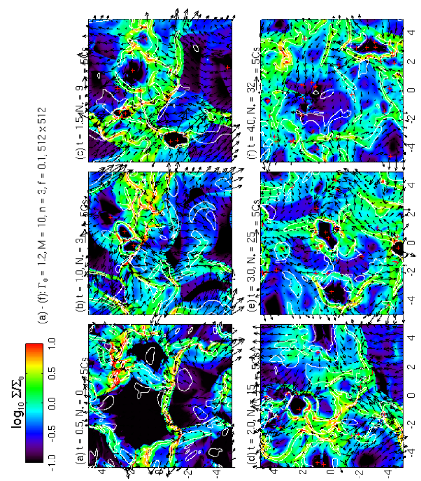
Figure 2.— Snapshots of the standard simulation at six representative times (given above each panel in units of $t_{g}$). Superposed on the color map of column density are velocity vectors (with normalization shown above each panel, where $C_{s}$ is the isothermal sound speed), contours of critical flux-to-mass ratio, and locations of the stars formed (denoted by crosses). The number of stars $N_{*}$ is given above each panel. The simulation box has 10 Jeans lengths ($L_{J}=0.37\ T_{10}/A_{V}$ pc) on each side.

Figure 3.— Mass fraction of the magnetically supercritical material (upper curve) created in the initially subcritical cloud of the standard simulation through ambipolar diffusion as a function of time. Only a fraction of this supercritical material resides in dense regions above ten times the average column density. The mass fraction of this dense, supercritical material is shown as the lower curve.

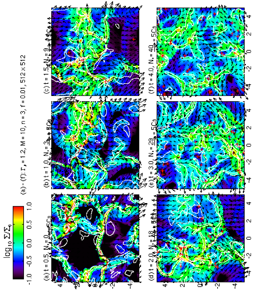
Figure 4.— Snapshots of a variant of the standard simulation with a weaker outflow of $f=0.01$ (Model S2 in Table 1). Superposed on the color map of column density are velocity vectors (with normalization shown above each panel, where $C_{s}$ is the isothermal sound speed), contours of critical flux-to-mass ratio, and locations of the stars formed (denoted by crosses). The number of stars $N_{*}$ is given above each panel. The simulation box has 10 Jeans lengths ($L_{J}=0.37\ T_{10}/A_{V}$ pc) on each side.

Figure 5.— Efficiencies of star formation of the six variants of the standard simulation listed in Table 1. The solid lines are for Models R1 and R2 that have the same power spectrum as the standard model, but different random realizations. The dotted lines are for Models I1 and I2 whose turbulent velocity fields are incompressible. The dashed (dash-dotted) line is for Model N1 (N2) that has a steeper (shallower) power spectrum than the standard model.

Figure 6.— Efficiencies of star formation for clouds of the same initial turbulent velocity field but different degrees of magnetization, measured by the dimensionless flux-to-mass ratio $\Gamma_{0}$ labeled beside the curves. The heavy (thin) solid lines are for strong (weak) outflow cases with $f=0.1$ (0.01).

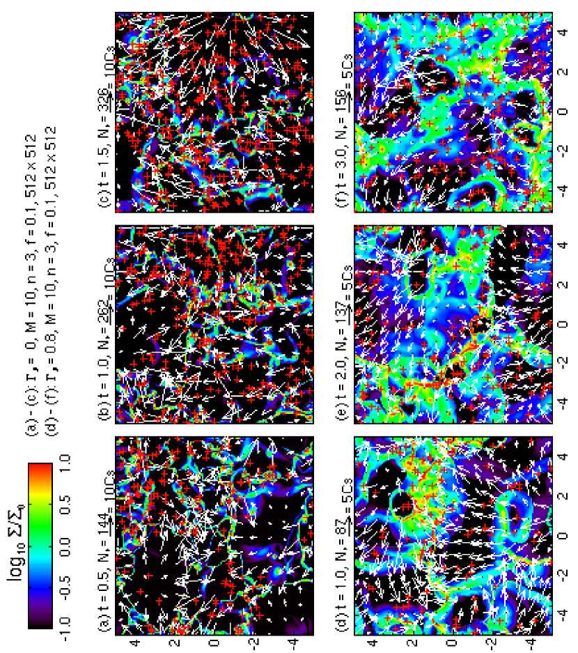
Figure 7.— Snapshots of a non-magnetic (Model O1; panels a-c) and marginally supercritical cloud with $\Gamma_{0}=0.8$ (Model U1; panels d-f) at three representative times (given above each panel in units of $t_{g}$). Superposed on the color map of column density are velocity vectors (with normalization shown above each panel, where $C_{s}$ is the isothermal sound speed) and locations of the stars formed (denoted by crosses). The number of stars $N_{*}$ is given above each panel. The simulation box has 10 Jeans lengths ($L_{J}=0.37\ T_{10}/A_{V}$ pc) on each side.

Figure 8.— Efficiencies of star formation for the standard subcritical cloud ($\Gamma_{0}=1.2$; solid lines) and a magnetically critical cloud ($\Gamma_{0}=1$; dotted lines) for different values of turbulent Mach number ${\cal M}$. The role of strong turbulence in accelerating star formation is evident.

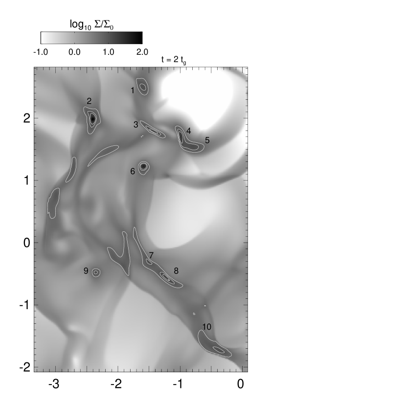
Figure 9.— Spatial distribution of the dense cores identified in the standard simulation at the time $t=2\ t_{g}$. The contours of column density are at $\Sigma=6,10$ and $14\ \Sigma_{0}$. Dense cores are enclosed by at least two contours. The core numbers are labeled.

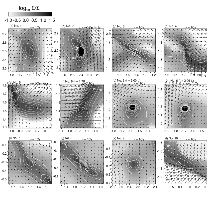
Figure 10.— Enlarged views of the dense cores shown in Fig. 9, except for panels (f) and (h), which display the core No.6 at two different times (labeled above the panels). Plotted in each panel are the contours of column density and vectors of the velocity relative to the density peak (marked by a cross). The velocity normalization is shown above each panel, where $C_{s}$ is the isothermal sound speed.

Figure 11.— The mass-weighted rms Mach numbers of the gas (solid line) and stars (dotted line) for the standard simulation as a function of time. Note the slowdown of turbulence decay at late times.

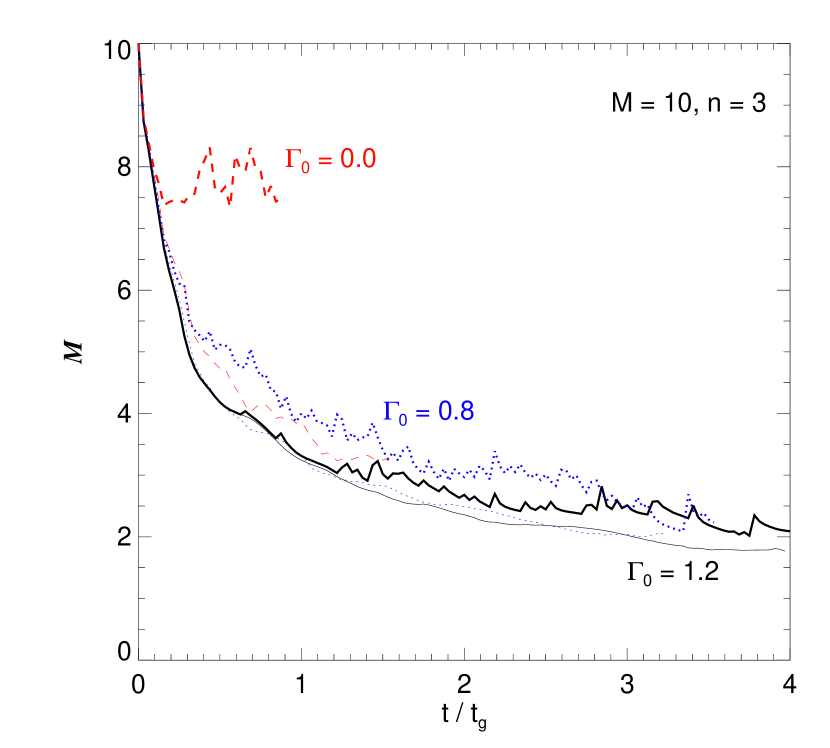
Figure 12.— The mass-weighted rms Mach numbers for the gas in the $\Gamma_{0}=1.2$ (subcritical; solid lines), 0.8 (supercritical; dotted lines) and 0 (non-magnetic; dashed lines) clouds as a function of time. The thick (thin) lines are for the strong (weak) outflow cases with $f=0.1\ (0.01)$. Evidently, appreciable replenishment of turbulence requires both a strong outflow and a high rate of star formation, a condition that is met only with the combination $\Gamma_{0}=0$ and $f=0.1$.

References

- Allen & Shu (2000) Allen, A. & Shu, F. H. 2000, ApJ, 536, 368
- Andre et al. (2000) Andre, P., Ward-Thompson, D., & Barsony, M. 2000, in Protostars and Planets IV, ed. V. Mannings, A. P. Boss, & S. S. Russell (Tuscon: Univ. Arizona Press), p. 59
- Arce & Goodman (1999) Arce, H. G. & Goodman, A. A. 1999, ApJ, 517, 264
- Ballesteros-Paredes et al. (2003) Ballesteros-Paredes, J., Klessen, R. S., & Vazquez-Semadeni, E. 2003, ApJ, 592, 188
- Basu & Ciolek (2004) Basu, S. & Ciolek, G. E. 2004, ApJ, 607, L39
- Basu & Mouschovias (1994) Basu, S. & Mouschovias, T. Ch. 1994, ApJ, 432, 720
- Bate et al. (2003) Bate, M. R., Bonnell, I. A., & Bromm, V. 2003, MNRAS, 339, 577
- Blitz & Williams (1999) Blitz, L. & Williams, J. 1999, in The Origins of Stars and Planetary Systems, ed. C. Lada & N. Kylafis (Kluwer), p.3
- Calvet (1997) Calvet, N. 1997, in Herbig-Haro Flows and the Birth of Stars, IAU Symposium No. 182, Edited by B. Reipurth and C. Bertout (Kluwer Academic Publishers), 1997, p. 417
- Crapsi et al. (2005) Crapsi, A., Caselli, P. & Walmsley, C. M. et al. 2005, ApJ, in press
- Crapsi et al. (2004) Crapsi, A., Caselli, P., & Walmsley, C. M., Tafalla, M., Lee, C. W., Bourke, T. L. 2004, A&A, 420, 957
- Crutcher (1999) Crutcher, R. M. 1999, ApJ, 520, 706
- Crutcher & Troland (2000) Crutcher, R. M. & Troland, T. H. 2000, ApJ, 537, 139
- Elmegreen & Scalo (2004) Elmegreen, B. G. & Scalo, J. 2004, ARAA, 42, 211
- Evans (1999) Evans, N. J., II, 1999, ARA&A, 37, 311
- Fatuzzo & Adams (2002) Fatuzzo, M. & Adams, F. C. 2002, ApJ, 570
- Fiedler & Mouschovias (1993) Fiedler, R. A. & Mouschovias, T. Ch. 1993, ApJ, 415, 680
- Gammie et al. (2003) Gammie, C. F., Lin, Y.-T., Stone, J. M., & Ostriker, E. C. 2003, ApJ, 592, 203
- Garrod et al. (2005) Garrod, R. T., Williams, D. A., Hartquist, T. W., Rawlings, J. M. C. & Viti, S. 2005, MNRAS, 356, 654
- Hartmann (2003) Hartmann, L. 2003, ApJ, 585, 398
- Hartmann et al. (2001) Hartmann, L., Ballesteros-Paredes, J., & Bergin, E. 2001, ApJ, 562, 852
- Heitsch et al. (2004) Heitsch, F., Zweibel, E. G., Slyz, A. D. & Devriendt, J. E. 2004, ApJ, 603, 165
- Hirota et al. (2002) Hirota, T., Ito, T., & Yamamoto, S. 2002, ApJ, 565, 359
- Hirsch (1990) Hirsch, C. 1990, Numerical Computation of Internal and External Flows Volume 2: Computational Methods for Inviscid and Viscous Flows (John Wiley & Sons), Chapters 20 and 21
- Hockney & Eastwood (1981) Hockney, R. W. & Eastwood, J. W. 1981, Computer Simulation using Particles (New York: McGraw Hill), p. 211
- Indebetouw & Zweibel (2000) Indebetouw, R. & Zweibel, E. G. 2000, ApJ, 532, 361
- Johnstone et al. (2004) Johnstone, D., Di Francesco, J. & Kirk, H. 2004, ApJ, L45
- Kenyon & Hartmann (1995) Kenyon, S. J. & Hartmann, L. 1995, ApJS, 101, 117
- Klessen et al. (2000) Klessen, R. S., Heitsch, F., & Mac Low, M.-M. 2000, ApJ, 535, 887
- Königl & Pudritz (2000) Königl, A., & Pudritz, R. E. 2000, in Protostars and Planets IV, ed. V. Mannings, A. P. Boss, & S. S. Russell (Tuscon: Univ. Arizona Press), p. 759
- Krasnopolsky & Gammie (2005) Krasnopolsky, R. & Gammie, C. F. 2005, ApJ, in press
- Lada et al. (2003) Lada, C. J., Bergin, E. A., Alves, J. & Huard, T. L. 2003, ApJ, 586, 286
- Lada & Lada (2003) Lada, C. J. & Lada, E. A. 2003, ARA&A, 41, 57
- Langer (1978) Langer, W. D. 1978, ApJ, 212, 39
- Larson (1981) Larson, R. B. 1981, MNRAS, 194, 809
- Larson (1985) Larson, R. B. 1985, MNRAS, 214, 379
- Lee et al. (1999) Lee, C. W., Myers, P. C. & Tafalla, M. 1999, ApJ, 526, 788
- Li et al. (2003) Li, P. S., Norman, M. L., Mac Low, M.-M., & Heitsch, F. 2004, ApJ, 605, 800
- Li & Nakamura (2002) Li, Z.-Y. & Nakamura, F. 2002, ApJ, 578, 256
- Li & Nakamura (2004) Li, Z.-Y. & Nakamura, F. 2004, ApJ, 609, L83
- Mac Low & Klessen (2004) Mac Low, M.-M. & Klessen, R. S. 2004, Rev. Mod. Phys., 76, 125
- Mac Low et al. (1998) Mac Low, M.-M., Klessen, R. S., Burkert, A., & Smith, M. D. 1998, Phys. Rev. Lett., 80, 2754
- Matzner & McKee (2000) Matzner, C. D. & McKee, C. F. 2000, ApJ, 545, 364
- McKee (1989) McKee, C. F. 1989, ApJ, 345, 782
- Mizuno et al. (1994) Mizuno, A., Onishi, T., Hayashi, M., Sunada, K., Hasegawa, T., & Fukui, Y. 1994, Nature, 368, 719
- Motte et al. (1998) Motte, F., Andre, P., & Neri, R. 1998, A&A, 336, 150
- Mouschovias & Ciolek (1999) Mouschovias, T. & Ciolek, G. 1999, in The Origins of Stars and Planetary Systems, ed. C. Lada & N. Kylafis (Kluwer), p. 305
- Mouschovias & Morton (1991) Mouschovias, T. Ch. & Morton, S. A. 1991, ApJ, 371, 296
- Myers & Fuller (1993) Myers, P. C. & Fuller, G. A. 1993, ApJ, 402, 528
- Myers & Khersonsky (1995) Myers, P. C. & Khersonsky, V. K. 1995, ApJ, 442, 186
- Myers et al. (1983) Myers, P. C., Linke, R. A. & Benson, P. J. 1983, ApJ, 264, 517
- Nakamura & Li (2002) Nakamura, F. & Li, Z.-Y. 2002, ApJ, 566, L101
- Nakamura & Li (2003) Nakamura, F. & Li, Z.-Y. 2003, ApJ, 594, 363
- Nakamura & Hanawa (1997) Nakamura, F. & Hanawa, T. 1997, ApJ, 480, 701
- Nakano (1984) Nakano, T. 1984, Fundamentals of Cosmic Physics, 9, 139
- Nakano (1998) Nakano, T. 1998, ApJ, 494, 587
- Nakano & Nakamura (1978) Nakano, T. & Nakamura, T. 1978, PASJ, 30, 671
- Nishi, Nakano, & Umebayashi (1991) Nishi, R., Nakano, T., & Umebayashi, T. 1991, ApJ, 368, 181
- Olmi & Testi (2002) Olmi, L. & Testi, L. 2002, A&A, 392, 1053
- Onishi et al. (2002) Onishi, T., Mizuno, A., Kawamura, A., Tachihara, K., & Fukui, Y. 2002, ApJ, 575, 950
- Ostriker et al. (1999) Ostriker, E. C., Gammie, C. F. & Stone, J. M. 1999, ApJ, 513, 259
- Padoan et al. (2001) Padoan, P., Juvela, M., Goodman, A. A. & Nordlund, A. 2001, ApJ, 533, 227
- Padoan & Nordlund (1999) Padoan, P. & Nordlund, A. 1999, ApJ, 526, 279
- Palla & Stahler (2002) Palla, F. & Stahler, S. 2002, ApJ, 581, 1194
- Scalo (1986) Scalo, J. M. 1986, Fundamentals of Cosmic Physics, 11, 1
- Shu (1991) Shu, F. H. 1991, The Physics of Astrophysics II (Mill Valley: University Science Books)
- Shu, Adams, & Lizano (1987) Shu, F. H., Adams, F. C., & Lizano, S. 1987, ARA&A, 25, 23
- Shu et al. (1999) Shu, F. H., Allen, A., Shang, H., Ostriker, E., & Li, Z.-Y. 1999, in The Origins of Stars and Planetary Systems, ed. C. Lada & N. Kylafis (Kluwer) p. 540
- Shu & Li (1997) Shu, F. H. & Li, Z.-Y. 1997, ApJ, 475, 251
- Shu et al. (2004) Shu, F. H., Li, Z.-Y. & Allen, A. 2004, ApJ, 601, 930
- Stone et al. (1998) Stone, J. M., Ostriker, E. C., & Gammie, C. F. 1998, ApJ, 508, L99
- Tafalla et al. (1998) Tafalla, M., Mardones, D., Myers, P. C., et al. 1998, ApJ, 504, 900
- Tafalla & Santiago (2004) Tafalla, M. & Santiago, J. 2004, A&A, 414, L53
- Valusamy & Langer (1998) Valusamy, T. & Langer, W. D. 1998, Nature, 392, 685
- Vazquez-Semadeni et al. (2005) Vazquez-Semadeni, E., Kim, J., Shadmehri, M., & Ballesteros-Paredes, J. 2005, ApJ, 618, 344
- Ward-Thompson et al. (1994) Ward-Thompson, D., Scott, P. F., Hills, R. E. & Andre, P. 1994, MNRAS, 268, 276
- Wolleben & Reich (2004) Wolleben, M. & Reich, W. 2004, A&A, 427, 537
- Zweibel (2002) Zweibel, E. G. 2002, ApJ, 567, 962