IRON K FEATURES IN THE QUASAR E 1821$+$643: EVIDENCE FOR GRAVITATIONALLY REDSHIFTED ABSORPTION?

Abstract

Abstract

We report a Chandra high-energy grating detection of a narrow, redshifted absorption line superimposed on the red wing of a broad Fe K line in the $z=0.297$ quasar E 1821$+$643. The absorption line is detected at a confidence level, estimated by two different methods, in the range $\sim 2-3\sigma$. Although the detection significance is not high enough to exclude a non-astrophysical origin, accounting for the absorption feature when modeling the X-ray spectrum implies that the Fe-K emission line is broad, and consistent with an origin in a relativistic accretion disk. Ignoring the apparent absorption feature leads to the conclusion that the Fe-K emission line is narrower, and also affects the inferred peak energy of the line (and hence the inferred ionization state of Fe). If the absorption line (at $\sim 6.2$ keV in the quasar frame) is real, we argue that it could be due to gravitationally redshifted Fe xxv or Fe xxvi resonance absorption within $\sim 10-20$ gravitational radii of the putative central black hole. The absorption line is not detected in earlier ASCA and Chandra low-energy grating observations, but the absorption line is not unequivocally ruled out by these data. The Chandra high-energy grating Fe-K emission line is consistent with an origin predominantly in Fe i–xvii or so. In an ASCA observation eight years earlier, the Fe-K line peaked at $\sim 6.6$ keV, closer to the energies of He-like Fe triplet lines. Further, in a Chandra low-energy grating observation the Fe-K line profile was double-peaked, one peak corresponding to Fe i–xvii or so, the other peak to Fe xxvi Ly$\alpha$. Such a wide range in ionization state of Fe is not ruled out by the HEG and ASCA data either, and is suggestive of a complex structure for the line-emitter.

Keywords: black hole physics – accretion disks – quasars: absorption lines – quasars: emission lines – quasars: individual (E 1821$+$643) – X-rays: galaxies

To appear in the Astrophysical Journal, 20 April 2005

1 INTRODUCTION

The high-luminosity ($L_{\rm 2-10\ keV}\sim 3-4\times 10^{45}\rm\ ergs\ s^{-1}$) quasar E 1821$+$643 ($z=0.297$) is one of the highest redshift quasars to exhibit strong Fe K$\alpha$ line emission. The source has been observed by every X-ray astronomy mission since EXOSAT, but until recently, the contribution to the Fe K$\alpha$ line emission from the cluster that the quasar is located in, was highly uncertain (e.g. see Saxton et al. 1997 and references therein). Fang et al. (2002) finally showed, from a Chandra observation, that the cluster makes a negligible contribution to line emission at 6.4 keV (the energy of Fe i $K\alpha$), and at most $\sim 3\%$ at Fe xxvi  Ly$\alpha$ ($\sim 6.9$ keV).

In this paper we show that one interpretation of the Chandra data for E 1821$+$643 is that the Fe K$\alpha$ emission line is relativistically broadened, with an absorption feature at $\sim 6.2$ keV (quasar frame) superimposed on the broad emission line profile. Whilst blueshifted absorption features are common in active galactic nuclei (AGNs), a redshifted absorption feature has been reported for only one case so far (NGC 3516, Nandra et al. 1999). The absorption feature in E 1821$+$643 could be due to resonance absorption in highly ionized Fe, in the form of an inflow, matter crossing the line-of-sight obliquely, or an outflow that is close enough to the putative central black hole that the absorption line suffers a strong gravitational redshift. The latter scenario would of course have very important implications for the study of the central engine with future missions. Whatever the origin of the absorption line, its presence in the HEG spectrum affects modeling of the Fe-K emission line at $\sim 6.4$ keV and therefore cannot be ignored. The absorption may be of a transitory nature since it is not detected in another Chandra observation, nor was it detected with ASCA. However, each of these latter data sets were not as sensitive to the absorption line and we will show that they do not unequivocally rule it out. Our analysis also shows a significant detection of Fe-K line emission at $\sim 6.9$ keV in Chandra low-energy grating (LEG) data (in addition to the line at $\sim 6.4$ keV). Likely to be associated with Fe xxvi Ly$\alpha$, this line is weak in the HEG data and not detected in the ASCA data, but both data sets are statistically consistent with the LEG data. The overall line profile in the ASCA data has a broad peak at $\sim 6.6$ keV but multiple emission lines cannot be resolved.

The paper is organized as follows. In §2 we describe the Chandra high-energy grating data and its reduction; in §3 we describe modeling of the Fe-K emission and absorption lines in these data, including a detailed discussion of the statistical significance of the absorption line. In §4 we discuss the Fe-K emission and absorption features with respect to two other important data sets for E 1821$+$643, namely from observations with the Chandra LEG and with ASCA. In §5 we discuss possibilities for the origin of the absorption line, and finally, in §6 we present our conclusions.

2 THE Chandra HEG DATA

E 1821$+$643 was observed with Chandra starting 9 February, 2001, from UT 14:28:55, for a duration of $\sim 100$ ks. This Chandra observation was made with the High-Energy Transmission Grating (or HETGS – Markert, et al. 1995) in the focal plane of the High Resolution Mirror Assembly. The Chandra HETGS affords the best spectral resolution in the $\sim 6-7$ keV Fe-K band currently available ($\sim 39$ eV, or $1860\rm\ km\ s^{-1}$ FWHM at 6.4 keV). HETGS consists of two grating assemblies, a High-Energy Grating (HEG) and a Medium-Energy Grating (MEG), and it is the HEG that achieves this spectral resolution. The MEG spectral resolution is only half as good as that of the HEG. The HEG also has a higher effective area in the Fe-K band, so our study will focus principally on the HEG data. The HEG and MEG energy bands are 0.4–10 keV and 0.7–10 keV respectively, but the effective area falls off rapidly with energy near both ends of each bandpass. The Chandra data were processed with version R4CU5UPD14.1 of the processing software, CALDB version 2.2 was used, and the telescope responses made using ciao 2.1.3. Otherwise, HEG and MEG lightcurves and spectra were made exactly as described in Yaqoob et al. (2003a). We used only the first orders of the grating data (combining the positive and negative arms, unless otherwise stated). The zeroth order data were piled up and the higher orders contain much fewer counts than the first order. The mean count rates (in the full energy band of each grating), over the entire Chandra observation were $0.1346\pm 0.0023$ ct/s and $0.2938\pm 0.0027$ ct/s for HEG and MEG respectively. HEG and MEG spectra extracted over the entire observation, resulted in a net exposure time of 99.620 ks. Background was not subtracted since it is negligible in the energy region of interest. The source flux showed little variability over the entire duration of the campaign. For example, for HEG plus MEG lightcurves binned at 1024 s, the excess variance above the expectation for Poisson noise (e.g. see Turner et al. 1999) was $(-0.4\pm 3.5)\times 10^{-4}$, consistent with zero.

Figure 1: The HEG spectrum of E 1821$+$643 (corrected for instrumental response), binned at $0.04\AA$. The source redshift is 0.297. The solid line is the best-fitting power-law model fitted over the observed energy range 1.0–2.0, 2.5–9 keV (omitting the 2.0–2.5 keV region where the mirror response is not well modeled). The energy range 1–9 keV corresponds to 1.3–11.7 keV in the rest-frame. The inset shows the ratio of the same spectrum to the above power-law model in the Fe K region. An asymmetric, broad Fe-K line is apparent, with a deep absorption feature superimposed on the profile. The vertical dotted lines correspond (from left to right) to the energies of the following transitions: Fe i K$\alpha$, Fe xxv $1s^{2}-1s2p$ forbidden and resonance lines, and Fe xxvi  Ly$\alpha$ (which correspond to rest-frame energies of 6.400, 6.636, 6.700, and 6.966 keV respectively).

3 SPECTRAL FITTING OF THE BROAD Fe-K EMISSION LINE AND NARROW ABSORPTION LINE

We used XSPEC v11.2 for spectral fitting (Arnaud 1996), omitting the 2–2.5 keV band due to systematic residuals around sharp changes in the effective area of the telescope – see Yaqoob et al. (2003a). The response matrices acisheg1D1999-07-22rmfN0004.fits and acismeg1D1999-07-22rmfN0004.fits (for the HEG and MEG respectively), combined with the telescope response files described above, were used to fold models through the instrument response and thereby directly compare predicted and observed counts spectra. Therefore, quoted fit parameters do not need to be corrected for instrumental response. For fitting purposes, the HEG and MEG spectra were binned at $0.01\AA$ and $0.02\AA$ respectively. The bin size is comparable to the FWHM spectral resolution ($0.012\AA$ and $0.023\AA$ for HEG and MEG respectively). For clarity, spectral plots in this paper show larger bin sizes than were used in the fitting (the bin size will be given case by case).

Since some energy bins may contain zero or few counts, the $C$-statistic was used for minimization and, unless otherwise stated, all statistical errors correspond to 90% confidence for one interesting parameter ($\Delta C=2.706$). By definition, calculation of the $C$-statistic requires only knowledge of the number of counts in a bin, but for spectral plots, the error bars shown correspond to asymmetric errors calculated using the approximations of Gehrels (1986). All model parameters will be referred to the source frame using $z=0.297$, unless otherwise stated.

We fitted the HEG spectrum in the 1–9 keV band, in the observed frame (except for the 2–2.5 keV band). Galactic absorption was not included in the model fitting since it has a negligible effect above 1 keV. First we fitted a simple power-law model. This model is shown in Fig. 1 overlaid on HEG data that have been corrected for the instrument resolution and binned at $0.04\AA$. The inset in Fig. 1 shows the ratio of data to model. It can be seen that there is broad, asymmetric excess emission centered around $\sim 4.9$ keV ($\sim 6.4$ keV quasar frame), likely corresponding to a low-ionization state Fe K$\alpha$ line. A similar, but narrower emission line has been reported by Fang et al. (2002) using the same data. However, there also appears to be a deep absorption feature, up to about $0.04\AA$ wide ($\sim 75$ eV at the observed energy), superimposed on the red wing of the emission line, at $\sim 4.8$ keV in the observed frame ($\sim 6.2$ keV in the quasar frame). The exact value of the centroid energy of the feature, and associated statistical errors, depend on the model of the emission line and these matters are discussed in §3.2 and §3.3.

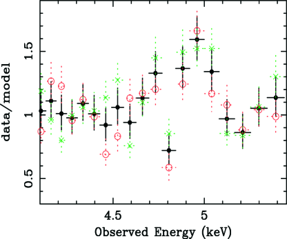
Figure 2: Detection of the high-energy absorption line in the separate $+1$ (green crosses) and $-1$ (red open circles) orders of the Chandra HEG, compared with the spectrum summed over both grating arms (black filled circles). The absorption line is probably due to redshifted He-like or H-like Fe absorption, equivalent to an inflow velocity of $\sim 2\times 10^{4}\ \rm km\ s^{-1}$ or $\sim 3\times 10^{4}\ \rm km\ s^{-1}$ respectively (see text). Shown are the ratios of spectral data (binned at $0.04\AA$) to the best-fitting power law fitted to the spectrum combined from both $+1$ and $-1$ orders of the grating (i.e. the same power-law model as shown in Fig. 1).

3.1 Reality of the Absorption Line

We investigated whether the apparent absorption line could be due to an instrumental artifact or a statistical fluctuation. We will describe this analysis in considerable detail since there are important physical consequences if the absorption line is real. Shown in Fig. 2 are the data/model ratios for the separate $+1$ and $-1$ orders, compared with the combined first-order data/model ratio (at bin sizes of $0.04\AA$), where the model is the simple power law fitted to the combined first-order data, as shown in Fig. 1 and described above. Fig. 2 shows that the absorption line is present, at some level, in both the negative and positive arms of the grating. Since the physical distance on the CCD detector of a photon event from the zeroth-order image determines the energy of that photon event, and the energy bin containing the absorption line in the negative and positive arms have completely different physical locations on the CCD array, an instrumental artifact cannot explain the absorption line. Also, the effective area of the HEG is smooth over the region the absorption line (centered on $\sim 4.8$ keV, observed frame) is detected: the combined $+1$ and $-1$ order effective area varies by no more than 6% over the observed energy range 4.6–5.0 keV. Yet the photon number in the $0.04\AA$ energy bin in which the line is observed, deviates by at least 40% compared to adjacent bins. A mis-calibration of the effective area would have to be present on extremely localized regions of different CCDs, corresponding to precisely the same energy bin. There are no other instrumental effects that we are aware of that could explain the absorption feature either.

To quantify the possibility that a statistical fluctuation occurred in both arms of the HEG, in the same energy bin, to conspire to yield an apparent absorption line like that observed, we employed two different methods to assess the statistical significance. The question we are seeking an answer to is the same in both cases. Namely, what is the probability of obtaining a statistical deviation in photon counts as large as that observed for the absorption line in one arm of the grating in any energy bin in the energy range searched, and then to observe a deviation as large as that measured in the other arm of the grating, this time in the same energy bin?

The first method we used is model-independent. For each first-order arm of the HEG, we calculated the fractional deviation of the counts in the $0.04\AA$ bin containing the absorption line, relative to the mean counts in the two bins either side of it. We must account for the total number of bins that were searched that resulted in the detection of the absorption feature, given that its energy does not correspond to a known atomic transition. For this, we used a very conservative assumption, counting all the energy bins that were used in spectral fitting. So, in the 1–2 keV and 2.5–9 keV range, for the $+1$ order, we calculated, for every bin, the Poisson probability of obtaining the same fractional deviation, say $X_{+}$ ($=58.1\%$), as for the absorption line in that arm. For this, we assumed the mean expected counts to be equal to the average of the two bins surrounding the target bin. Then, by combining these probabilities, we calculated the total probability of observing the deviation, $X_{+}$, in any of the energy bins in the energy range 1–2, 2.5–9 keV. Next, we calculated the probability in the other HEG arm ($-1$ order) of obtaining the observed deviation, $X_{-}$ ($=47.9\%$), in the actual absorption-line bin, relative to the average counts of the two surrounding bins. We obtained a final probability of obtaining the actual deviations that were observed, $X_{+}$ and $X_{-}$, in the $+1$ and $-1$ arms of the HEG respectively (and simultaneously), of $2.38\times 10^{-3}$ (i.e. this is the probability that both detections were due to statistical fluctuations). This corresponds to an overall significance of $3.04\sigma$ for detection of the absorption line.

We went further and estimated a significance using an even more conservative assumption. This was based on the possibility that both bins surrounding the absorption-line bin, in each HEG arm, could both have been higher than the expectation values, due to statistical fluctuations, thus artificially enhancing the depth of the absorption line. Therefore, we repeated the above calculations after reducing the counts in all bins by $1\sigma$, in both HEG arms, except for the counts in the absorption line bins. Here, we used $1+\sqrt{(0.75+N)}$ for the $1\sigma$ error on the counts, $N$ (see Gehrels 1986). Strictly speaking, this is not correct for small $N$, but the bins either side of the absorption line in each arm of the HEG have between 34 and 43 counts, so the effect of the approximation on the final result is unimportant. (Note that the MEG has between 17 and 29 counts per bin in the bins either side of the absorption line, in each arm). Using this more pessimistic prescription we get $1.95\sigma$ for the significance of the absorption line, which is consistent with the fact that we have effectively artificially reduced the level of the reference ‘continuum’ by $\sim 1\sigma$.

Table 1: Gaussian Line Fits to Chandra HEG Data for E 1821$+$643

Parameter	Measurement
$C$-statistic	1017.0
Degrees of freedom	968
Emission Line Center Energy (keV)	$6.31^{+0.06}_{-0.05}$
Emission Line Width, $\sigma$ (keV)	$0.18^{+0.05}_{-0.04}$
Emission Line Velocity	$20145^{+5800}_{-4625}$
(FWHM, $\rm km\ s^{-1}$)
Emission Line Intensity	$5.2^{+1.3}_{-1.2}$
($\rm 10^{-5}\ photons\ cm^{-2}\ s^{-1}$)
Emission Line EW (eV)	$296^{+74}_{-69}$
Absorption Line Center Energy	$6.228^{+0.011}_{-0.018}$
(keV)
Absorption Line Gaussian Width	$0.027^{+0.011}_{-0.007}$
$\sigma$ ( keV)
Absorption Line Velocity Width	$3040^{+1280}_{-780}$
(FWHM, $\rm km\ s^{-1}$)
Absorption Line Equivalent Width,	$54^{+12}_{-14}$
EW (eV)
Power-Law Photon Index $\Gamma$	$1.82^{+0.03}_{-0.03}$

Simple power-law model plus a Gaussian emission line, and a Gaussian absorption line, fitted to the Chandra HEG data (see §3.2 for details). All parameters (except 2–10 keV flux) are referred to the quasar frame ($z=0.297$). Errors are 90% confidence for one parameter ($\Delta C=2.706$). Velocities have been rounded to the nearest 5 $\rm km\ s^{-1}$.

The second method we used to assess the significance of the line employed Monte Carlo simulations. We took a model for the continuum and emission line, and folded it through the instrument response, so that we could measure deviations of the data relative to this model. We used the power-law plus Gaussian emission line model described in §3.2 and Table 1, and set the absorption line equivalent width (EW) in that model to zero. Obviously the probabilities calculated from the Monte Carlo simulations will depend somewhat on the model but we will see that the results are consistent with the model-independent method described above.

We measured negative deviations relative to the continuum plus emission-line model of 20.5% and 38.2% in photon counts, in the $0.04\AA$ energy bin containing the absorption line, in the $+1$ and $-1$ HEG orders respectively and used these as inputs to the Monte Carlo calculations. We ran $10^{6}$ simulations for every energy bin, for each HEG first-order arm. We used the most conservative assumption again, for the number of energy bins searched, namely the 1–2 and 2.5–9 keV range. We measured the deviations relative to the model, in each bin, and in each simulation, and thus obtained a final probability that the observed absorption line is due to chance statistical fluctuations, of $2.44\times 10^{-2}$, or a significance of $2.25\sigma$. This is consistent with the estimate of 2–3 $\sigma$ from the model-independent method described above. We note that these are all very conservative estimates of the significance, because in principle, we could have found the absorption line in the real data by examining a smaller number of energy bins.

From Fig. 1, it might appear as if there are deviations as strong, or stronger, than those for the reported absorption line, notably at $\sim 2.5$ keV, and above $\sim 6$ keV (both observed frame). We remind the reader that 2–2.5 keV is the region of greatest changes in effective area, mainly due to the X-ray telescope (XRT), so even small inaccuracies in the calibration of the effective area can result in apparent emission or absorption features. Indeed, one finds that the deviations at $\sim 2.5$ keV are not consistent in the $+1$ and $-1$ HEG arms. In fact, we already mentioned in §3 that we did not use the 2–2.5 keV data in any of our analysis or simulations, due to the difficult calibration of this region of the XRT response.

On the other hand, the deviations above $\sim 6$ keV in the $+1$ and $-1$ HEG orders do correlate with each other and may represent real structure. For example, Fe-K edges are in the right energy range (6 keV corresponds to $\sim 7$ keV in the quasar frame). However, the effective area of the HEG (and MEG) drops quickly above 6 keV, and the statistical significance of these deviations is much less than that of the reported absorption line, and is not sufficient to warrant further investigation.

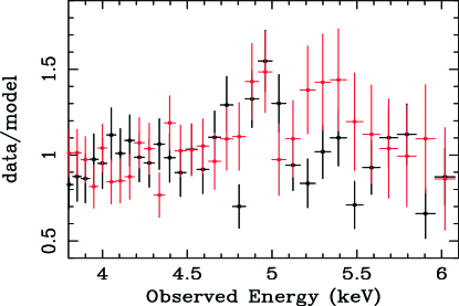
Figure 3: A comparison of the HEG data (black) with the MEG data (red) in the Fe-K region in E 1821$+$643. Shown are the ratios of spectral data (binned at $0.04\AA$) to the best-fitting power-law fitted to the HEG spectrum combined from both $+1$ and $-1$ orders of the HEG (i.e. the same power-law model as shown in Fig. 1 and Fig. 2). Although the absorption line does not appear to be significantly detected in the MEG, the probability of obtaining more counts than expected in the absorption-line bin by chance (assuming the HEG absorption-line equivalent width is the mean of a Poisson distribution), is 46.4%. Therefore the MEG data do not rule out an absorption line.

We also investigated whether the absorption line is detected in the MEG data. A direct comparison of the MEG and HEG data is given in Fig. 3. Shown are the ratios of MEG and HEG data to a simple power-law continuum fitted in the 1.0-2.0, 2.5–9 keV bands. Although no absorption line is evident in the MEG data, it is worth remembering that the MEG effective area is a factor 1.5 less than that of the HEG at the energy at which the HEG absorption line is detected. We quantified the probability that the MEG would not detect the absorption line, given the HEG measurements. The observed number of counts in the $0.04\AA$ bin that would contain the absorption line in the MEG spectrum is 43. Taking the best-fitting HEG power-law plus Gaussian emission line, and absorption-line model (see §3.2) and folding it through the MEG instrumental response function, and fitting for the overall cross-normalization difference between HEG and MEG ($\sim 8\%$), we estimated the mean expected counts in the absorption-line bin to be 32.2. The difference between expected and measured counts in that bin is only $\sim 1.1\sigma$. The Poisson probability of actually obtaining 33 or more counts in that bin is then 46.6%. In other words, this is the probability that the MEG would observe an absorption line that is apparently weaker than that measured by the HEG. An alternative way of expressing the fact that the HEG and MEG data are consistent with each other is that the probability of measuring between 33–43 counts in the absorption-line bin in the MEG is 44.1%.

We conclude that the significance of the absorption line is not low enough to unequivocally attribute it to a statistical artifact, but neither is the significance high enough to ascribe to an astrophysical origin without caution. As we show below, the absorption line is significant enough to affect modeling of the Fe-K emission line, so it cannot be ignored.

3.2 Gaussian Emission-Line Model

Here we describe fitting the HEG data (combined from the $+1$ and $-1$ order spectra) with a power-law plus Gaussian emission line, with and without an absorption line included. If we do not include an absorption line, we obtain Gaussian Fe-K emission-line parameters entirely consistent with those measured by Fang et al. (2002). Namely, we obtained a center energy of $6.43^{+0.06}_{-0.05}$ keV, a Gaussian width of $0.10^{+0.07}_{-0.03}$ keV, and an EW of $144^{+67}_{-57}$ eV (all parameters in the quasar frame). Note that the EW given by Fang et al. (2002) is in the observer’s frame so must be multiplied by $(1+z)$ in order to directly compare with ours.

On the other hand, if an inverted Gaussian is included to model the absorption line, the emission line parameters are different, because there is some apparent emission redward of the absorption line, that is not modeled when the absorption line is not included. This is because a single Gaussian model worsens the fit if it is extended over the apparent absorption in the data, so it remains narrow. The power-law plus emission and absorption-line model involves a total of eight free parameters, and their best-fitting values and statistical errors are shown in Table 1. It can be seen that, compared with an emission-line only model, the peak energy of the emission line shifts down by $\sim 150$ eV, and the intrinsic width is larger, because when the an absorption line model is included, there is excess emission on the red side of the absorption line that is modeled as part of the emission line. Also, since some of the emission line is absorbed, a larger intrinsic intensity and EW are required.

Figure 4: Joint, two-parameter confidence contours (68%, 90%, and 99%) for the equivalent width (EW) and FWHM of the high-energy absorption-line feature in E 1821$+$643 when the broad Fe K$\alpha$ emission line is modeled in terms of a Gaussian (s olid contours) and in terms of relativistic disk line (dotted contours). The absorption line is modeled with an inverted Gaussian in both cases. In the quasar frame the center energy of the absorption line is $6.228^{+0.011}_{-0.018}$ keV (Gaussian emission line) or $6.220^{+0.018}_{-0.013}$ keV (disk emission line). Details of all model parameters are given in Table 1 and Table 2. The contours were obtained from spectral fitting to the HEG data (summed over $+1$ and $-1$ orders).

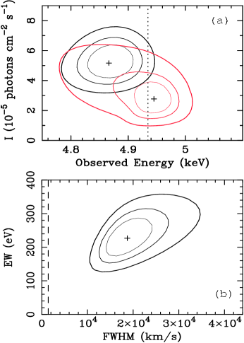
Figure 5: (a) Contours corresponding to joint two-parameter confidence levels of 68%, 90%, and 99% for the intensity and center energy (observed frame) of the broad Fe K$\alpha$ line in E 1821$+$643 when it is modeled with a simple Gaussian. Black contours correspond to the case when an inverted Gaussian is included to model the absorption line in the HEG data (see Fig. 4) and red contours to the case when the absorption line is omitted from the model and these contours are entirely consistent with Fig. 4 of Fang et al. (2002). Caption is abridged: full caption given at the end of this article.

Fig. 4 shows the joint two-parameter 68%, 90%, and 99% confidence level contours of the absorption line EW versus its FWHM. The width depends somewhat on how the emission-line is modeled (see §3.3 for further discussion). For a Gaussian emission line model, the FWHM is $\sim 3000\rm\ km\ s^{-1}$ (see Table 1). Fig. 5 (a) shows the joint two-parameter 68%, 90%, and 99% confidence level contours of the Gaussian emission-line intensity versus observed center energy, directly comparing the two cases, with (black), and without (red) an absorption line included in the model. The (red) contours, for the model with no absorption line, are consistent with those obtained by Fang et al. (2002), but note that ours are plotted against observed energy in Fig. 5 (a), but the same contours are shown against quasar-frame energy, in Fig. 9. Fig. 5 (b) shows the EW of the emission line versus its FWHM (when the absorption line is included in the model). When modeled with a Gaussian, the emission line has a FWHM of $\sim 20000\rm\ km\ s^{-1}$ (see Table 1).

We note that Fang et al. (2002) reported the detection, albeit marginal, of an additional emission line at $6.94^{+0.05}_{-0.07}$ keV, very likely due to Fe xxvi Ly$\alpha$. Using combined HEG and MEG data they obtained a $\Delta C$ of 9.2 upon the addition of a three-parameter Gaussian to model the line, corresponding to a confidence level of 97.3%. Fang et al. (2002) measured a line intensity and EW of $1.1\pm 0.7\times 10^{-5}\ \rm photons\ cm^{-2}\ s^{-1}$ and $64\pm 40$ eV respectively (we have corrected the EW values of Fang et al. for cosmological redshift). Only an upper limit was obtained for the intrinsic width, 0.15 keV. Using the same model as Fang et al. (i.e. a power law plus two Gaussians with no absorption line included), we obtained consistent results for the high-energy iron line from the HEG and MEG data. Namely, a similar detection significance (98.0%), a center energy of $6.94\pm 0.04$ keV, a line intensity of $0.8^{+0.7}_{-0.5}\times 10^{-5}\rm\ photons\ cm^{-2}\ s^{-1}$, an EW of $40^{+35}_{-25}$ eV, and an intrinsic width of $0.03^{+0.05}_{-0.02}$ keV. All statistical errors, ours and those of Fang et al. (2002) quoted here for the high-energy iron line are 90% confidence for one interesting parameter.

Table 2: Relativistic Disk Line Fits to Chandra HEG Data for E 1821$+$643

Parameter	Measurement
$C$-statistic	1014.5
degrees of freedom	966
Disk Line Rest Energy (keV)	$6.57^{+0.01}_{-0.01}$
	(6.51–6.68)
Disk Line Emissivity Index, $q$	$2.69^{+0.19}_{-0.19}$
	(2.36–3.08)
Outer Disk Radius, $R_{\rm out}$	$>930$
	($>18$)
Disk Inclination, $\theta_{\rm obs}$ (degrees)	$0.0^{+0.4}_{-0.0}$
	(0–27)
Disk Line Intensity ($\rm 10^{-5}\ photons\ cm^{-2}\ s^{-1}$)	$7.0^{+1.9}_{-1.7}$
	(3.6–10.2)
Disk Line EW (eV)	$209^{+51}_{-57}$
	(107–305)
Absorption Line Center Energy (keV)	$6.220^{+0.018}_{-0.013}$
Absorption Line Gaussian Width, $\sigma$ (keV)	$0.021^{+0.012}_{-0.008}$
Absorption Line Velocity Width, FWHM ($\rm km\ s^{-1}$)	$2385^{+1440}_{-950}$
Absorption Line Equivalent Width, EW (eV)	$34^{+13}_{-13}$
Power-Law Photon Index, $\Gamma$	$1.84^{+0.03}_{-0.03}$
2–10 keV Observed Flux ($10^{-11}\rm\ ergs\ cm^{-2}\ s^{-1}$)	1.2
2–10 keV Luminosity, Quasar Frame ($10^{45}\rm\ ergs\ s^{-1}$)	3.3

Simple power-law model plus a relativistic disk emission line, and a Gaussian absorption line, fitted to the Chandra HEG data (see §3.3 for details). All parameters (except 2–10 keV flux), refer to the quasar frame ($z=0.297$). Errors are 90% confidence for one parameter ($\Delta C=2.706$); 90% confidence, five-parameter ranges are also given for the disk line parameters (i.e. $\Delta C=9.24$) in parentheses. Velocities have been rounded to the nearest 5 $\rm km\ s^{-1}$. Intrinsic luminosity, in the 2–10 keV band in the quasar frame, calculated using $H_{0}=70\rm\ km\ s^{-1}\ Mpc^{-1}$ and $\Lambda=0.7$.

3.3 Absorption Line Plus Relativistic Disk Line Model

Since the Fe-K line emission appears to be asymmetric and peaks below 6.4 keV ($6.31^{+0.06}_{-0.05}$ keV, from Table 1), we replaced the Gaussian emission line in the model described above, with a model of an Fe K$\alpha$ emission line originating in a Keplerian disk rotating around a Schwarzschild black hole (e.g. Fabian et al. 1989). The inner radius of emission was fixed at $6r_{g}$ ($r_{g}\equiv GM/c^{2}$) and the outer radius was a free parameter. The line radial emissivity was assumed to be a power law (line intensity proportional to $r^{-q}$), with the index, $q$, free. In the disk rest-frame the emission-line energy was allowed to vary between the Fe K$\alpha$ line energies for Fe i and Fe xxvi, allowing a $\sim 10$ eV margin on either side (i.e. 6.39–6.98 keV). The disk inclination angle and overall line intensity were also free parameters. Thus, there were a total of five free parameters for the disk line model.

The best-fitting parameters of the absorption line, disk emission line, and the continuum are shown in Table 2, and the best-fitting model is shown in Fig. 6 (a). The counts spectrum with the best-fitting model folded through the instrument response and overlaid on the data is shown in Fig. 6 (b), whilst Fig. 6 (c) shows the ratio of the data to the best-fitting model. Note that since the $C$-statistic varied erratically (for $|\Delta C|<5$) for some of the disk line parameters, Table 2 also shows the 90% confidence, five-parameter ranges (i.e. $\Delta C=9.24$). The quasar-frame absorption-line parameters from the fit are $6.220^{+0.018}_{-0.013}$ keV (center energy), $21^{+12}_{-8}$ eV (Gaussian width), and $34\pm 13$ eV (equivalent width, or EW). Fig. 4 shows joint two-parameter confidence contours for the EW versus FWHM of the absorption line (dotted contours), directly compared with the contours obtained when the emission line was modeled with a Gaussian (§3.2). The absorption-line parameters are a little different for the two cases, (notably, the absorption-line EW is smaller when the emission is modeled with a disk line).

Figure 6: (a) Best-fitting power-law plus disk emission-line model for the HEG data for E 1821$+$643, including an inverted Gaussian for the absorption line. (b) HEG counts spectrum (summed over $+1$ and $-1$ orders), with the best-fitting model (solid line) in (a) overlaid on the data, after folding through the instrument response. (c) Ratio of the spectral data to the best-fitting model in (b). In both (b) and (c) the spectra are binned at $0.04\AA$.

We compare our best-fitting disk line parameters to those of Fang et al. (2002). Our inclination angle (zero degrees) appears to be smaller, but since $C$ varies erratically around this best-fitting angle, when one considers the 90%, five-parameter upper limit (27 degrees), our result is consistent with that of Fang et al. (2002), who obtained $21.5^{+6.9}_{-10.4}$ degrees. Our EW of $209^{+51}_{-57}$ eV is consistent with that obtained by Fang et al. (2002), who obtained $168^{+59}_{-72}$ eV, which has to be be multiplied by $(1+z)$ in order to correct for cosmological redshift. We do, however, require a larger line flux in order to compensate for the absorption line included in the model. We fitted the disk-line model without the absorption line and obtained a line intensity of $4.3^{+1.4}_{-1.4}\times 10^{-5}\ \rm\ photons\ cm^{-2}\ s^{-1}$, consistent with the Fang et al. (2002) value of $3.2^{+1.1}_{-1.4}\times 10^{-5}\ \rm\ photons\ cm^{-2}\ s^{-1}$ (again, Fang et al. did not correct for cosmological redshift so their value has to be increased by 1.297 before comparing with ours).

Although the signal-to-noise of the HEG data is limited, the data are quite sensitive to the disk inclination angle not being too large and the disk outer radius not being too small. If the inclination angle is much greater than $\sim 30^{\circ}$, and/or the outer radius much less than $\sim 20r_{g}$, then the disk line would be too broad to fit the data. We note that the inclusion of a Compton-reflection continuum to the model described above has a negligible effect on the disk line parameters because the additional component is not required ($|\Delta C|<1$) due to poor statistics at the high-energy end of the spectrum. For solar abundances, we obtain a 90% confidence, one-parameter upper limit on the solid angle of the reflector of $0.7(2\pi)$. For an Fe abundance of three times solar, this upper limit is $0.95(2\pi)$. Ionization of the disk and/or inclusion of relativistic smearing effects increases this upper limit but still has no effect on the line parameters because structure in the continuum produced by Compton reflection that could potentially affect the line parameters, is not required by the data.

4 Fe-K EMISSION & ABSORPTION IN OTHER DATA SETS

There are two other principal data sets for E 1821$+$643 that we can examine in order to compare with the Chandra HETGS data, namely data from observations with the Chandra low-energy grating spectrometer (LETGS) and ASCA. Except for a BBXRT observation, that was very short, and in which the Fe-K emission line was barely detected (Yaqoob et al. 1993), all observations of E 1821$+$643 prior to the ASCA observation were made with proportional counters, which had poor spectral resolution. E 1821$+$643 has not been observed by XMM-Newton (although it is present, but too far off-axis, in an observation pointed at a nearby brown dwarf). Below we describe results from observations with the Chandra LETGS and ASCA in turn.

4.1 Chandra LEG Observation

E 1821$+$643 was observed by the Chandra low-energy grating spectrometer (LETGS) in 2001, January 17–24, resulting in a deep exposure of this object. Although the low-energy grating (LEG) has a spectral resolution of only $0.05\AA$ FWHM (or $\sim 150$ eV at 6 keV), it has an effective area a factor of $\sim 2$ larger than that of the HEG at the observed energy of the line. The ACIS CCDs were used as the detector for the gratings in this observation. The low-energy spectrum from this observation has been discussed by Mathur et al. (2003), but details of the Fe-K complex from this data set have not been discussed in the literature. We obtained a net exposure time of 470.8 ks, and the source showed negligible flux variability during the entire observation.

Figure 7: Comparison of the Fe-K complex in E 1821$+$643 between non-contemporaneous Chandra HEG, Chandra LEG, and ASCA (SIS) data (see §4). Shown are the ratios of data to a simple power-law model. Caption is abridged: full caption given at the end of this article.

The ratio of the LEG data (around the Fe-K region), to a single power law fitted over the 1–2, 2.5–9 keV observed energy interval, is shown in Fig. 7. An estimate of the line profile itself, with the above continuum subtracted off is shown in Fig. 8. The latter plot also shows the LEG data directly compared with the HEG data, showing that the overall line flux in the HEG is somewhat larger. It can be seen that there are two apparent emission peaks in the LEG data, not one. One peak is centered near 6.4 keV (quasar frame) and the other near the energy of the Fe xxvi  Ly$\alpha$ transition, which is at 6.966 keV (rest energy). The second emission-line peak in the LEG data occurs across several resolution elements and is present in both the $+1$ and $-1$ orders of the grating data. It also has a high statistical significance: the difference in the fit statistic between a single and double-Gaussian model for the line emission is 18.3 (for two additional free parameters in the double-Gaussian model).

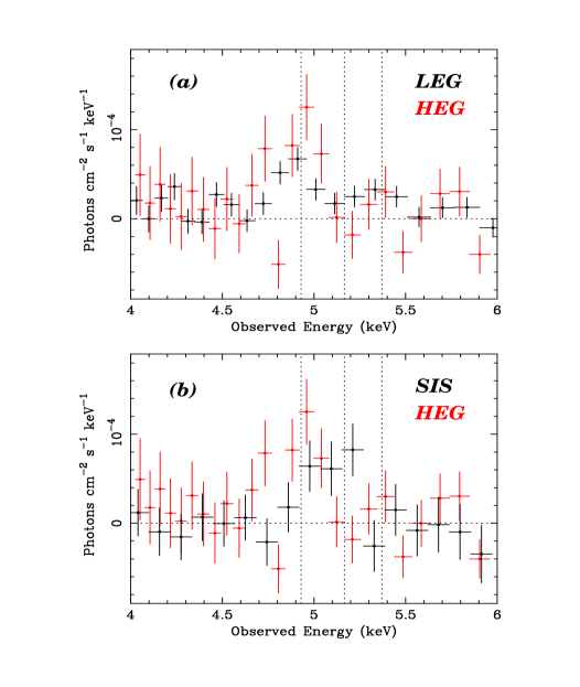
Figure 8: Comparison of the Fe-K complex in E 1821$+$643 between non-contemporaneous Chandra HEG, Chandra LEG, and ASCA (SIS) observations (see §4). Shown are the absolute fluxes after the best-fitting power-law continua (as fitted in Fig. 7) are subtracted. Therefore, these plots can be used to assess absolute intensity changes in the line emission. (a) Chandra LEG data (black) compared directly with the Chandra HEG data (red). (b) ASCA SIS data (black) compared directly with the Chandra HEG data (red).

Table 3 shows the best-fitting parameters and their statistical errors, obtained from fitting a power-law plus double-Gaussian model to the LEG data. It can be seen that the energies of the emission-line peaks are very well constrained. The fact that the first and second emission-line peaks in the LEG data are consistent with the energies of K lines from Fe i and Fe xxvi respectively, suggests that they are two separate emission lines, rather than a single, broad, disk line profile.

It would appear that the Fe-K emission-line profile measured from the LEG is different to that measured from the HEG data. However, as pointed out in §3.2, Fang et al. (2002) reported marginal evidence for a peak near the energy of Fe xxvi  Ly$\alpha$ in the Chandra HEG data, which we confirmed (§3.2) and which can be seen in our Chandra HEG spectrum (e.g. Fig. 1). In fact, formally, the intensity of the high-energy iron emission line measured by the HEG is statistically consistent with that measured by the LEG (compare HEG values in §3.2 with LEG values in Table 3).

No absorption line at the position seen in the HEG data is evident in the LEG data. However we can obtain an upper limit on the EW of an absorption line if it were present, and had the center energy and width of the line observed in the HEG (see Table 1). We added an inverted Gaussian with the HEG parameters to the double-Gaussian emission-line model and obtained an upper limit on the EW of the absorption line of 23 eV, to be compared with the HEG values of $54^{+12}_{-14}$ and $34^{+13}_{-13}$ eV, corresponding to Gaussian and disk-line models of the Fe-K emission, respectively (all values are in the quasar frame). Thus, the LEG data do not rule out the presence of the absorption line if the disk-line model is more appropriate for the emission line than the Gaussian model. Moreover, strictly speaking, a one-parameter 90% upper limit for the LEG absorption-line EW is not appropriate since there are a total of eight free parameters in the model (plus a continuum normalization). The 90%, eight-parameter upper limit on the LEG included in the HEG model, then the 99% HEG and LEG contours do not overlap. Therefore, it is possible that the lower-energy peak in the Fe-K line profile varied between the HEG and LEG observations.

4.2 ASCA Observation

E 1821$+$643 was observed by ASCA in 1993, June 19 and the results of this observation have been discussed by Yamashita et al. (1997). We reanalyzed the data, in a manner similar to that described in Weaver, Gelbord, & Yaqoob (2001). We restricted our analysis to the two CCD Solid State Imaging Spectrometers (SIS) since they had much better spectral resolution than the Gas Imaging Spectrometers (GIS) aboard ASCA. At 6 keV, the spectral resolution of the SIS was $\sim 150$ eV FWHM at the time of the observation. We combined data from the two SIS detectors and obtained a net exposure time of 83.4 ks. We used $\chi^{2}$ statistics for fitting the data since the counts per bin are much higher than in the Chandra grating spectra, and background has to be subtracted for ASCA data.

The ratio of the SIS data to a single power law fitted over the 1–9 keV observed energy interval is shown in Fig. 7. This plot also shows the ASCA data directly compared with the HEG data. An estimate of the line profile itself, with the above continuum subtracted off is shown in Fig. 8. The latter plot also shows the ASCA data directly compared with the HEG data, showing that the line appears to peak at a different energy in each observation. It can be seen that there is a broad emission peak in the ASCA data, centered near the He-like Fe triplet transitions ($\sim 6.6-6.7$ keV in the quasar frame).

Table 3: Double Gaussian Line Fits to Chandra LEG Data for E 1821$+$643

Parameter	Measurement
$C$-statistic	256.2
Degrees of freedom	187
$E_{1}$, First Emission Line Rest Energy (keV)	$6.35^{+0.03}_{-0.05}$
$I_{1}$, First Line Intensity ($\rm 10^{-5}\ photons\ cm^{-2}\ s^{-1}$)	$1.40^{+0.35}_{-0.30}$
$EW_{1}$, First Emission Line Equivalent Width (eV)	$89^{+23}_{-19}$
$E_{2}$, Second Emission Line Rest Energy (keV)	$6.91^{+0.09}_{-0.09}$
$I_{2}$, Second Emission Line Intensity ($\rm 10^{-5}\ photons\ cm^{-2}\ s^{-1}$)	$0.82^{+0.31}_{-0.34}$
$EW_{2}$, Second Emission Line Equivalent Width (eV)	$61^{+23}_{-26}$
$\sigma$, Gaussian Emission Line Widths (keV)	$0.12^{+0.06}_{-0.03}$
FWHM of Emission Lines ($\rm km\ s^{-1}$)	$13350^{+5050}_{-4140}$
Absorption Line Equivalent Width, EW (eV)	$0^{+23}_{-0}$
Power-Law Photon Index, $\Gamma$	$1.87^{+0.01}_{-0.01}$
2–10 keV Observed Flux ($10^{-11}\rm\ ergs\ cm^{-2}\ s^{-1}$)	1.0
2–10 keV Luminosity, Quasar Frame ($10^{45}\rm\ ergs\ s^{-1}$)	2.7

Simple power-law model plus two Gaussian emission lines fitted to the Chandra low-energy grating (LEG) data (see Fig. 7, Fig. 8, Fig. 9, and §4.1 for details). All parameters (except 2–10 keV flux) refer to the quasar frame ($z=0.297$). Errors are 90% confidence for one parameter ($\Delta C=2.706$). The emission-line velocity widths (forced to be the same for the two lines) were frozen for deriving the error ranges on the other parameters, otherwise the fits became unstable. The EW of a Gaussian absorption line added to the above model is also given, where the center energy and width of the absorption line are fixed at the respective values obtained from the HEG data (see Table 1). Velocities have been rounded to the nearest 5 $\rm km\ s^{-1}$. Intrinsic luminosity, in the 2–10 keV band in the quasar frame, was calculated using $H_{0}=70\rm\ km\ s^{-1}\ Mpc^{-1}$ and $\Lambda=0.7$.

Table 4 shows the results of fitting the ASCA data with a power-law plus Gaussian emission-line model. The center energy of the line is $6.62^{+0.12}_{-0.12}$ keV, and the EW is $140^{+78}_{-86}$ eV (both in the quasar frame). The fitted to the Chandra low-energy grating (LEG) data (see Fig. 7, Fig. 8, Fig. 9, and §4.1 for details). All parameters (except 2–10 keV flux) refer to the quasar frame ($z=0.297$). Errors are 90% confidence for one parameter ($\Delta C=2.706$). The emission-line velocity widths (forced to be the same for the two lines) were frozen for deriving the error ranges on the other parameters, otherwise the fits became unstable. The EW of a Gaussian absorption line added to the above model is also given, where the center energy and width of the absorption line are fixed at the respective values obtained from the HEG data (see Table 1). Velocities have been rounded to the nearest 5 $\rm km\ s^{-1}$. Intrinsic luminosity, in the 2–10 keV band in the quasar frame, was calculated using $H_{0}=70\rm\ km\ s^{-1}\ Mpc^{-1}$ and $\Lambda=0.7$.

Table 4 shows the results of fitting the ASCA data with a power-law plus Gaussian emission-line model. The center energy of the line is $6.62^{+0.12}_{-0.12}$ keV, and the EW is $140^{+78}_{-86}$ eV (both in the quasar frame). The line is unresolved with ASCA. Our results are consistent with those of Yamashita et al. (1997), who obtained a center energy of $6.58\pm 0.05$ keV and an EW of $100\pm 50$ eV (both in the quasar frame). Fig. 9 shows the 68%, 90%, and 99% contours of line intensity versus line energy obtained from Gaussian-fitting of the emission line in the ASCA data, compared with confidence contours obtained from the HEG and LEG data. It can be seen that the 99% confidence contours obtained from modeling the principal line peak in the HEG and ASCA data overlap (with or without an absorption line included in the HEG model). Therefore, at 99% confidence, we cannot exclude the case that the HEG and ASCA emission-line profiles are consistent with each other. At 99% confidence, the LEG contours for the peak at $\sim 6.4$ keV also overlap with the ASCA contours. Although the emission line at $\sim 6.9$ keV is not detected in the ASCA data, the presence of such a line with the same energy and width as the in the LEG data is not ruled out by the ASCA data. Adding such an additional Gaussian emission line to the ASCA data, even the 90%, one-parameter upper limit on the intensity, $1.3\times 10^{-5}\ \rm photons\ cm^{-2}\ s^{-1}$, is consistent with the LEG intensity ($0.8^{+0.3}_{-0.3}\times 10^{-5}\ \rm photons\ cm^{-2}\ s^{-1}$; see Table 3).

In order to test the ASCA data for the absorption line found in the HEG data, we added an inverted Gaussian to our power-law plus single Gaussian emission-line model in order to obtain an upper limit on the EW of an absorption line with energy and width fixed at the values obtained from the HEG data (see Table 1). There were now a total five free parameters, plus a continuum normalization. The 90%, one-parameter and five-parameter upper limits on the EW are 82 eV and 138 eV (quasar frame) respectively. Thus, the ASCA data do not rule out the presence of an absorption line that has the parameters that were measured by the Chandra HEG.

We also modeled the emission line in the ASCA data with a relativistic disk-line model, as was fitted to the HEG data in §3.3. Since the spectral resolution and signal-to-noise of the data are limited, we fixed $r_{\rm in}=6r_{g}$, $r_{\rm out}=1000r_{g}$, and $q=2$. The line energy in the disk frame, its intensity, and the disk inclination angle were free parameters. We obtained a best-fitting line energy of $6.71^{+0.10}_{-0.16}$ keV (in the disk frame), and an EW of $161^{+89}_{-67}$ eV (in the quasar frame), but obtained only an upper limit on the inclination angle, of $30^{\circ}$ (90%, one-parameter). The inclination angle upper limit is consistent with the inclination angle inferred from disk-line fits to the HEG data (§3.3). However, the ASCA data strongly constrain the line energy in the disk frame to be near that expected for He-like Fe triplet emission (between $\sim 6.6$–6.7 keV). The HEG data constrained the line energy to values appropriate for $K\alpha$ transitions from much lower ionization states of Fe (i.e. Fe i–Fe xvii or so). This is not surprising since the HEG data are strongly peaked near 6.4 keV, whilst the ASCA data are strongly peaked near 6.6 keV (quasar-frame quantities).

With the above ASCA disk-line model, we obtained a somewhat smaller upper limit on the EW of an absorption line with the parameters measured from the HEG data, namely $53$ eV (90% confidence, one-parameter).

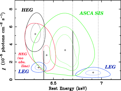
Figure 9: Direct comparison of joint, two-parameter, 68%, and 99% confidence contours of emission-line intensity, $I$, versus line energy between non-contemporaneous Chandra HEG, Chandra LEG, and ASCA (SIS) data (see §4). For ASCA, 90% confidence contours are also shown. In each case the data were modeled with a simple power law and a Gaussian emission line (two in the case of the LEG in order to model the two peaks - see Fig. 7). The black HEG contours were obtained when an inverted gaussian was included to model the absorption feature (the same contours are shown in Fig. 5). The red HEG contours were obtained with no absorption feature included (as were the LEG and ASCA contours). The ASCA emission line can also be modeled as two discrete, unresolved lines at 6.4 keV and 6.7 keV, and the 99% two-parameter ranges on the line intensities for this scenario are shown as solid vertical bars at those energies (also see Fig. 10). Caption is abridged: full caption given at the end of this article.

Figure 10: The ASCA emission line in E 1821$+$643 can be modeled as two discrete, unresolved lines at 6.4 keV and 6.7 keV, corresponding to Fe i K$\alpha$, Fe xxv $1s^{2}-1s2p$ resonance transitions respectively (see §4.2 for details). Shown are the joint, two-parameter, 68%, 90%, and 99% confidence contours of the intensity of the 6.7 keV line ($I_{6.7}$) versus the intensity of the 6.4 keV line ($I_{6.4}$). It can seen that the 6.4 keV line is not required at $>90\%$ confidence but is allowed to have an intensity high enough to be present at the level detected in either the HEG or LEG data (see Fig. 9).

An alternative description of the ASCA data is that there are two, narrow, unresolved emission lines. We fitted a dual-Gaussian model for the line emission, with the line widths free but forced to be the same value for the two lines. We fixed the energy of one line at 6.40 keV (Fe i $K\alpha$), and that of the other line at 6.70 keV (Fe xxv resonance, $1s^{2}-1s2p$). We obtained equivalent widths of $42^{+37}_{-33}$ eV, and $87^{+54}_{-34}$ eV respectively (quasar frame). The lower and upper bounds on the line intensities from this model are shown in Fig. 9, along with intensity versus energy contours for the Gaussian models fitted to HEG, LEG, and ASCA data, as described in previous sections. Fig. 10 shows the 68%, 90%, and 99% joint confidence contours of the intensity of one line versus the other from the dual-Gaussian model for two unresolved lines in the ASCA data. Fig. 10 shows that, in this model, the 6.7 keV line dominates the line profile since the 6.4 keV is not actually required at 99% confidence and higher. We obtained an upper limit of 8,400 $\rm km\ s^{-1}$ FWHM on the width of the lines in the dual-Gaussian model.

5 ORIGIN OF THE ABSORPTION LINE

If the absorption line at $\sim 6.2$ keV detected in the HEG data is real, variability is a possible explanation of non-detection of the absorption line in the ASCA and LEG data (but we recall that neither of these data sets unequivocally rule out the absorption line). If the absorption line is real, it could be due to a redshifted resonance transition in highly ionized Fe. The high ionization state would be consistent with the fact that we find no significant soft X-ray absorption features in the HEG data (see also Fang et al. 2002), and Mathur et al. (2003) came to a similar conclusion about the LEG data. If the HEG absorption line were due to blueshifted absorption from lighter elements, one would expect absorption features from other ionic species, particularly Fe. If the line is due to a $K\alpha$ transition from Fe xxv or Fe xxvi, the observed redshift then corresponds to a recession velocity of $20750^{+585}_{-810}\ \rm km\ s^{-1}$ or $32130^{+560}_{-780}\ \rm km\ s^{-1}$ respectively (see Yaqoob et al. 2003b and references therein for the sources of atomic data that we use). At the very least, $v/c\sim 3\%$, or $\sim 9380\ \rm km\ s^{-1}$ (corresponding to Fe i).

At face value, one could interpret the absorption-line redshift of $\sim 2-3\times 10^{4}\rm\ km\ s^{-1}$ as inflow (e.g. onto the putative central black hole). To derive a recession velocity one would have to account for gravitational redshifts (at the unknown radial distances). Evidence for inflow is very rare, and in the X-ray band, only one other case has been reported (in NGC 3516, Nandra et al. 1999). In that case inflow was not the only interpretation (e.g. see Ruszkowski & Fabian 2000) and neither is it for the present case of E 1821$+$643.

Another interpretation is that the absorption line is due to highly-ionized material that is crossing the line-of-sight obliquely and may, for example, have have been ejected from the accretion disk (a similar scenario for line emission was considered for Mkn 766 by Pounds et al. 2003a and Turner, Kraemer, and Reeves 2004). If the ejected blob still has the Keplerian motion of the disk then from the redshift and upper limit on the absorption line width, one can derive a lower limit on the radial distance from the black hole since, in a given observation time, the blob cannot travel too far or else the absorption line would be too broad. This gives a constraint on the minimum radial distance of the absorption site from the central black hole, as a function of the disk inclination angle. This scenario predicts that the absorption line energy and EW should be significantly variable.

Yet another possibility is that the redshift of the absorption line is gravitational in origin. The absorber could of course be outflowing and yet still give an overall redshift, if it is close enough to the putative central black hole. From pure gravitational redshifts alone, one can place a limit on the allowed range of distances, $r$, from the black hole that can be occupied by the absorbing gas. To first order, from a given line width $\Delta E$, $\Delta r\sim r(r/r_{g})(\Delta E/E_{0})$, where $E_{0}$ is the rest energy of the line. For $r=10r_{g}$, $\Delta E\sim 50$ eV, and $E_{0}\sim 7$ keV, we have $\Delta r\sim r_{g}$. Obviously, the actual allowed range of radii required to keep the absorption line narrow depends on the details of the geometry of the X-ray source and of the kinematics of the absorber (whether inflow or outflow). The detailed kinematics of the flow, its physical state (e.g. ionization, density, temperature), and its proximity to the putative black hole will all affect the line width. Nevertheless, $\Delta r$ is rather small. However, we note that the quasar model of Elvis (2000) involves a cylindrical outflow (that could intercept the X-ray continuum over a narrow range of radii). Reports of outflows in AGN are now common, and a few are claimed to originate within tens to hundreds of gravitational radii of the central black hole (e.g. Pounds et al. 2003b, 2003c). However, it has been claimed that many of these outflows may not exist if absorption features that are really local to our Galaxy have been misidentified as being at the redshift of the AGN (McKernan, Yaqoob, & Reynolds 2005).

Table 4: Gaussian Line Fits to ASCA SIS Data for E 1821$+$643

Parameter	Measurement
$\chi^{2}$	168.6
Degrees of freedom	266
Emission Line Rest Energy (keV)	$6.62^{+0.12}_{-0.12}$
Emission Line Intensity	$3.4^{+1.9}_{-2.1}$
($\rm 10^{-5}\ photons\ cm^{-2}\ s^{-1}$)
Emission Line Equivalent Width	$140^{+78}_{-86}$
(eV)
$\sigma$, Gaussian Emission Line Width	$0.14^{+0.16}_{-0.14}$
(keV)
FWHM of Emission Line ($\rm km\ s^{-1}$)	$14935^{+17660}_{-14935}$
Absorption Line Equivalent Width,	$4^{+78}_{-4}$
EW (eV)
Power-Law Photon Index, $\Gamma$	$1.80^{+0.03}_{-0.02}$
2–10 keV Observed Flux	1.6
($10^{-11}\rm\ ergs\ cm^{-2}\ s^{-1}$)
2–10 keV Luminosity,	4.3
Quasar Frame ($10^{45}\rm\ ergs\ s^{-1}$)

Simple power-law model plus Gaussian emission line fitted to the ASCA SIS data (see Fig. 7, Fig. 8, Fig. 9, and §4.2 for details). All parameters (except 2–10 keV flux) refer to the quasar frame ($z=0.297$). Errors are 90% confidence for one parameter ($\Delta C=2.706$). The EW of a Gaussian absorption line added to the above model is also given, where the center energy and width of the absorption line are fixed at the respective values obtained from the HEG data (see Table 1). Velocities have been rounded to the nearest 5 $\rm km\ s^{-1}$. Intrinsic luminosity, in the 2–10 keV band in the quasar frame, was calculated using $H_{0}=70\rm\ km\ s^{-1}\ Mpc^{-1}$ and $\Lambda=0.7$.

6 CONCLUSIONS

During a Chandra HETGS observation of E 1821$+$643 we detected an absorption line, at a significance level of $2-3\sigma$, at $\sim 6.2$ keV in the quasar frame. Whether or not this absorption line is accounted for in modeling the Fe-K emission line, directly affects the inferred width of the emission line and its peak energy. We have also found that the Fe-K emission-line spectra of E 1821$+$643 during observations with the Chandra HETGS, Chandra LETGS, and ASCA appear at first to be different to each other. The first two observations were separated by $\sim 3$ weeks and the ASCA observation was made nearly eight years earlier. The 2–10 keV luminosity of E 1821$+$643 during the ASCA and HETGS observations was only $\sim 60\%$, and $\sim 20\%$ higher, respectively, than during the LETGS observation. The Fe-K line profile during the ASCA observation was peaked at $\sim 6.6$ keV, during the HETGS observation it was strongly peaked at $\sim 6.4$ keV, and during the LETGS observation the line profile was double-peaked, at $\sim 6.4$ keV, and $\sim 6.9$ keV (all are quasar-frame energies). These properties of the Fe-K line region are captured in Fig. 7, Fig. 8, and Fig. 9. However, due to limited signal-to-noise, a non-varying Fe-K complex cannot be ruled at 99% confidence. It is possible that $K\alpha$ emission from from Fe i–xvii or so, He-like Fe, and Fe xxvi  Ly$\alpha$ is present with similar intensities in all three data sets. However, it will be extremely important to test for variability in the Fe-K emission complex with future missions.

Clearly, the structure of the line-emitter must be complex (for example, there may be more than one emitter), in order to produce this range in Fe ionization states simultaneously (e.g. emission lines from Fe i-xvii and Fe xxvi are detected with a high significance in the LETGS data). However, the location of the line-emitting region or regions is not known. Certainly, in the HETGS data the Fe-K line at $\sim 6.4$ keV could be broad, indicating an origin close to the putative black hole, such as an accretion disk. The spectral resolution of the ASCA and LEG data is insufficient to ascertain whether the emission lines during these observations were narrow or broad, although it appears that during the LETGS observation the lines were not as broad as the line observed during the HETGS observation.

The putative absorption line detected by the high energy grating (HEG) on the Chandra HETGS is not unequivocally ruled out by any of the data sets. We argue that if the absorption line is real, it is most likely due to redshifted resonance absorption in either He-like or H-like Fe. The origin of the redshift (equivalent to $v/c\sim 0.066-0.106$), could be absorption in highly ionized matter that is either inflowing or crossing the line-of-sight obliquely. In the latter case the material could be due to ejecta from the accretion disk. A more controversial interpretation is that the absorption line is due to an outflow that is so close to the black hole ($<15r_{g})$, that the absorption line is gravitationally redshifted. If this is true then we would have an important new diagnostic for studying strong gravity, complementing studies using the Fe K$\alpha$ emission lines.

AstroE-2, with a factor of $\sim 6$ greater effective area than the Chandra HEG at the relevant energies, and a spectral resolution of $\sim 6$ eV, will help to constrain the origin of the Fe-K emission features in E 1821$+$643, and provide a more sensitive search for absorption lines of the kind found in the HEG data.

TY gratefully acknowledges support from NASA grants NNG04GB78A and NAG5-10769, and AR4-5009X, the latter issued by the Chandra X–ray Observatory Center, operated by the SAO for and on behalf of NASA under contract NAS8–39073. This research made use of the HEASARC online data archive services, supported by NASA/GSFC and also of the NASA/IPAC Extragalactic Database (NED) which is operated by the Jet Propulsion Laboratory, California Institute of Technology, under contract with NASA. The authors are grateful to the Chandra instrument and operations teams, and to Urmila Padmanabhan for help with some of the analysis.

FULL FIGURE CAPTIONS

Figure 5 (Full Caption)
(a) Contours corresponding to joint two-parameter confidence levels of 68%, 90%, and 99% for the intensity and center energy (observed frame) of the broad Fe K$\alpha$ line in E 1821$+$643 when it is modeled with a simple Gaussian. Black contours correspond to the case when an inverted Gaussian is included to model the absorption line in the HEG data (see Fig. 4) and red contours to the case when the absorption line is omitted from the model and these contours are entirely consistent with Fig. 4 of Fang et al. (2002). The red contours are shown again in Fig. 9 of the present paper, in that case plotted against quasar-frame energy, and these are directly comparable with Fig. 4 of Fang et al. (2002). Excluding the absorption line results in a slightly higher peak energy for the emission line. The vertical dotted line corresponds to 6.4 keV in the quasar frame. (b) As (a) for the equivalent width (EW) and FWHM of the broad Fe K$\alpha$ line. The dashed line corresponds to the HEG FWHM spectral resolution at the observed peak energy of the broad line, and shows that the Fe K$\alpha$ line is resolved by the HEG. The absorption line is included in the model (see Fig. 4). See §3.2 and Table 1 for details.

Figure 7 (Full Caption)
Comparison of the Fe-K complex in E 1821$+$643 between non-contemporaneous Chandra HEG, Chandra LEG, and ASCA (SIS) data (see §4). Shown are the ratios of data to a simple power-law model, fitted to each data set in the 1–9 keV observed energy range (excluding the 2–2.5 keV interval for the HEG and LEG data). It can be seen that the line profile in each case appears to be different, with the LEG profile showing two peaks (but see §4.1 and §4.2 for a quantitative assessment of variability). The vertical dotted lines correspond (from left to right) to the energies of the following transitions: Fe i K$\alpha$, Fe xxv $1s^{2}-1s2p$ resonance, and Fe xxvi  Ly$\alpha$ (that correspond to rest-frame energies of 6.400, 6.700, and 6.966 keV respectively). It can be seen that the HEG profile peaks near Fe i K$\alpha$, the LEG peaks are near Fe i K$\alpha$ and Fe xxvi Ly$\alpha$, whilst the ASCA peak is near the Fe xxv triplet resonance line energy.

Figure 9 (Full Caption)
Direct comparison of joint, two-parameter, 68%, and 99% confidence contours of emission-line intensity, $I$, versus line energy between non-contemporaneous Chandra HEG, Chandra LEG, and ASCA (SIS) data (see §4). For ASCA, 90% confidence contours are also shown. In each case the data were modeled with a simple power law and a Gaussian emission line (two in the case of the LEG in order to model the two peaks - see Fig. 7). The black HEG contours were obtained when an inverted gaussian was included to model the absorption feature (the same contours are shown in Fig. 5). The red HEG contours were obtained with no absorption feature included (as were the LEG and ASCA contours). The red HEG contours are consistent with, and directly comparable with those shown in Fig. 4 of Fang et al. (2002). The vertical dotted lines correspond (from left to right) to the energies of the following transitions: Fe i K$\alpha$, and Fe xxv $1s^{2}-1s2p$ resonance, and Fe xxvi  Ly$\alpha$ (that correspond to rest-frame energies of 6.400, 6.700, and 6.966 keV respectively). At 99% confidence the evidence for variability in the total line intensity between LEG and HEG (i.e. for LEG this means the sum of the two lines) is marginal, and the ASCA 99% contours are large enough to overlap all the other contours. The ASCA emission line can also be modeled as two discrete, unresolved lines at 6.4 keV and 6.7 keV, and the 99% two-parameter ranges on the line intensities for this scenario are shown as solid vertical bars at those energies (also see Fig. 10).

References

- [1] Arnaud, K. A. 1996, Astronomical Data Analysis Software and Systems V, eds. Jacoby, G., & Barnes, J., p. 17, ASP Conference Series, Vol. 101
- [2] Elvis, M. 2000, ApJ, 545, 63
- [3] Fang, T., Davis, D. S., Lee, J. C., Marshall, H. M., Bryan, G. L., & Canizares, C. R. 2002, ApJ, 565, 86
- [4] Fabian, A. C., Rees, M. J., Stella, L., & White, N. E. 1989, MNRAS, 238, 729
- [5] Gehrels, N. 1986, ApJ, 303, 336
- [6] Markert, T. H., Canizares, C. R., Dewey, D., McGuirk, M., Pak, C., & Shattenburg, M. L. 1995, Proc. SPIE, 2280, 168
- [7] Mathur, S., Weinberg, D. H., & Chen, X. 2003, ApJ, 582, 82
- [8] McKernan, B., Yaqoob, T., & Reynolds, C. S. 2005, ApJ, 617, 232
- [9] Nandra, K., George, I. M., Mushotzky, R. F., Turner, T. J., & Yaqoob, T. 1999, ApJ, 523, L17
- [10] Pounds, K. A., King, A. R., Page, K. L., O’Brien, P. T. 2003b, MN, 346, 1025
- [11] Pounds, K. A., Reeves, J. N., King, A. R., Page, K. L., O’Brien, P. T., & Turner, M. J. L. 2003c, MN, 345, 705
- [12] Pounds, K. A., Reeves, J. N., Page, K. L., Wynn, G. A., O’Brien, P. T. 2003a, MN, 342, 1147
- [13] Ruszkowski, M., & Fabian, A. C. 2000, MN, 315, 223
- [14] Saxton, R. D., Barstow, M. A., Turner, M. J. L., Williams, O. R., Stewart, G. C., & Kii, T. 1997, MN, 289, 196
- [15] Turner, T. J., George, I. M., Nandra, K., & Turcan, D. 1999, ApJ, 524, 667
- [16] Turner, T. J., Kraemer, S. B., & Reeves, J. N. 2004, ApJ, 603, 62
- [17] Weaver, K. A., Gelbord, J., & Yaqoob, T. 2001, ApJ, 550, 261
- [18] Yamashita, A., Matsumoto, C., Ishida, M., Inoue, H., Kii, T., & Makishima, K. 1997, ApJ, 486, 763
- [19] Yaqoob, T., Serlemitsos, P. J., Mushotzky, R. F., Weaver, K. A., Marshall, F. E., & Petre, R. 1993, ApJ, 418, 638
- [20] Yaqoob, T., George, I. M., Kallman, T. R., Padmanabhan, U., Weaver, K. A., & Turner, T. J. 2003b, ApJ, 596, 85
- [21] Yaqoob, T., McKernan, B., Kraemer, S. B., Crenshaw, D. M., Gabel, J. R., George, I. M., & Turner, T. J. 2003a, ApJ, 582, 105