New Catalogs of Compact Radio Sources in the Galactic Plane
Abstract
Archival data have been combined with recent observations of the Galactic plane using the Very Large Array to create new catalogs of compact centimetric radio sources. The 20 cm source catalog covers a longitude range of ; the latitude coverage varies from to . The total survey area is deg2; coverage is 90% complete at a flux density threshold of mJy, and over 5000 sources are recorded. The 6 cm catalog covers 43 deg2 in the region to a 90% completeness threshold of 2.9 mJy; over 2700 sources are found. Both surveys have an angular resolution of . These catalogs provide a 30% (at 20 cm) to 50% (at 6 cm) increase in the number of high-reliability compact sources in the Galactic plane, as well as providing greatly improved astrometry, uniformity, and reliability; they should prove useful for comparison with new mid- and far-infrared surveys of the Milky Way.
Subject headings:
surveys — catalogs — Galaxy: general — radio continuum: ISM — H II regions — supernova remnants1. Introduction
Between 1982 and 1991, the Very Large Array (VLA)111The National Radio Astronomy Observatory is operated by Associated Universities, Inc. under cooperative agreement with the National Science Foundation was used to conduct extensive snapshot surveys along the plane of the Milky Way at both 6 and 20 cm. In a series of papers in the early 1990s (Becker et al. 1990; Zoonematkermani et al. 1990; White et al. 1991; Helfand et al. 1992; Becker et al. 1992; Becker et al. 1994), we presented catalogs of over 4000 compact () radio sources, and used the best far-infrared observations then available (IRAS) to construct large samples of compact and ultracompact H II regions, planetary nebule, etc. Although we employed the best data reduction practices available and tractable on the computers of that era, the images themselves and the source catalogs derived from them left much to be desired. Nonetheless, these data remain the most sensitive radio survey in existence for compact radio emitters in the Galactic plane. The Midcourse Space Experiment (MSX) mid-infared survey of the plane (Price et al. 2001; Egan, Price, and Kramer 2003) offers significant improvement in both sensitivity and angular resolution over the largely source-confused IRAS images, and the recent launch of the Spitzer Space Telescope presages extensive new mid- and far-IR observations of the Milky Way. These developments warrant a new look at the available radio data.
Thus, we have carried out a complete re-reduction of the archival VLA data, supplementing the individual pointings with 28 hours of new observations designed to correct deficiencies in the existing database. This paper presents new, improved images and catalogs of discrete radio sources at both 6 and 20 cm, as well as unveiling a new Web site that makes all the images publicly accessible.
We have also undertaken a new multi-configuration 20 cm VLA map of the Milky Way (D. J. Helfand et al., 2005, in preparation). The new images are of much higher quality than any previous radio observations of the Galactic plane, but they cover only a portion of the plane () at a single wavelength. The older VLA data complement the new survey by extending its area and frequency coverage. While the analysis of the new data is not yet complete, we use it in this paper in several checks of the quality of the images and catalogs presented here.
In section 2 we provide a description of the observations included in this project, while §3 describes our data analysis, highlighting the differences between the original reductions and our current efforts. The source catalogs, containing over 10,000 entries, comprise §4, where we also provide descriptions of a number of tests we have performed to quantify the surveys’ astrometric and photometric accuracies, as well as highlighting the caveats essential for making productive use of these data. §5 introduces the Galactic plane Web site (http://third.ucllnl.org/gps), which allows easy access to all images and catalogs, and describes some of the uses to which these data products can (and will) be put.
2. Observations
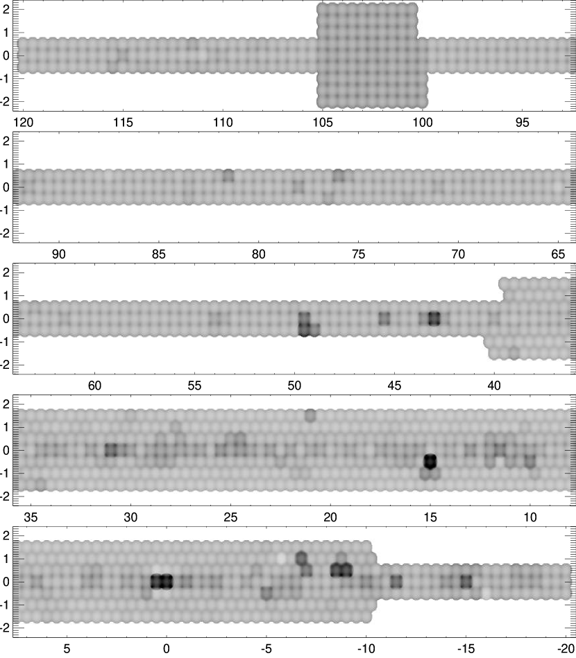
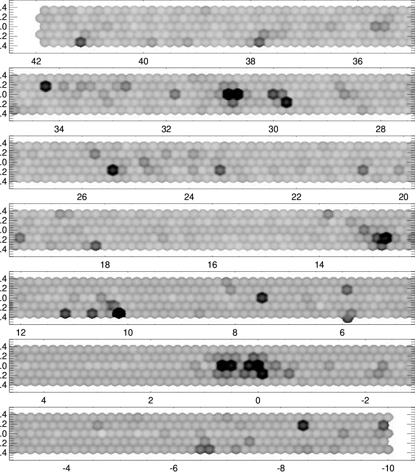
The observations used to construct the catalogs presented herein were taken for a variety of purposes over a period of twenty-two years in seven of the eight possible VLA configurations. The 20 cm data acquired by other authors between 1982 and 1986 were on a rectilinear grid that provided less-than-optimal coverage (see Fig. 1). Beginning in 1989, we sought, through a series of proposals, to fill out the 20 cm coverage in the Galactic center region and the first two quadrants, and to complement these data in the inner Galaxy with a 6 cm snapshot survey. Some of the latter data were corrupted when taken in the original C-configuration and the observations were repeated in 1991, albeit in the lower-resolution DnC and D configurations. Furthermore, some of the maps constructed from the salvagable 1990 data were compromised by very bright, extended sources. Given the continuing utility of our compact source catalogs, we reobserved both the low-resolution and compromised fields in the Spring 2004 C-configuration; these data replace the respective 1990–1991 data in the current analysis. We also observed a single field at 20 cm in February 2005 to fill in the only remaining hole in the 20 cm coverage.
All of our analysis reported in this paper focuses on the total intensity maps; we have not attempted to analyze the available polarization data. The 20 cm observations were mainly taken in line mode to avoid the bandwidth smearing problems that accompany wide-field continuum imaging at that wavelength. Such data do not have associated polarization information, so the available 20 cm polarization data have incomplete sky coverage. The 6 cm observations were taken in continuum mode and could be used to construct polarization images, but they would likely be of limited value because most of the 6 cm Galactic emission is expected to be thermal and unpolarized. Another obstacle is that the data do not include observations of polarization standard calibration sources. Nonetheless, it might be interesting for a future study to use these same data to examine the polarization properties of Galactic radio sources.
The 20 cm observations taken in 1983 used one IF bandpass at 1611 MHz that included a strong OH maser line. Becker, White & Proctor (1992) used these data to construct a catalog of OH masers. For this paper we are interested in radio continuum emission, but it is necessary in the data analysis to account for the OH masers. The self-calibration particularly is complicated by the possibility that a source may have very different flux densities in the two IFs (see §3.1 below for further discussion.)
A summary of the observations used in our final analysis is presented in Table 1. We include the observation dates, configuration, number of fields observed, Galactic longitude range covered, number of bands and bandwidths used, and the central observing frequencies. Most snapshots were of approximately 90-s duration. Over 110 hours of observing time are represented by these observing programs (including fields not used in our final images.) The coverage is complete at 20 cm over the range ; the latitude coverage ranges from to . The 6 cm coverage is complete in the region . Total sky coverage is approximately 331 deg2 and 43 deg2 at 20 cm and 6 cm, respectively. Figure 1 displays coverage maps in a grayscale format that illustrates the different extents, pointing grids, and sensitivities of the two surveys.
| Date | Config | # fields | range | channels | freq |
|---|---|---|---|---|---|
| (deg) | (MHz) | (MHz) | |||
| 20 cm Observations | |||||
| 20 Jul 1982 | B | 96 | 100–105 | 1 6 | 1443 |
| 24 Dec 1983 | BnA | 31 | 340–0 | 2 3 | 1441/1611 |
| 27 Dec 1983 | BnA | 79 | 340–0 | 2 3 | 1441/1611 |
| 30 Dec 1983 | BnA | 241 | 340–0 | 2 3 | 1441/1611 |
| 24 Jul 1986 | B | 194 | 0–100 | 2 3 | 1441/1641 |
| 25 Jul 1986 | B | 193 | 0–100 | 2 3 | 1441/1641 |
| 23 Mar 1989 | B | 29 | 340–50 | 2 3 | 1465/1515 |
| 27 Mar 1989 | B | 42 | 105–120 | 2 3 | 1465/1515 |
| 29 Apr 1989 | B | 1 | 357.5 | 2 3 | 1465 |
| 01 May 1989 | B | 199 | 350–40 | 14 3 | 1465 |
| 02 May 1989 | B | 203 | 350–40 | 14 3 | 1465 |
| 01 Feb 2005 | BnA | 1 | 354.25 | 2 25 | 1451/1490 |
| Total | 1309 | ||||
| 6 cm Observations | |||||
| 22 Jun 1989 | C | 228 | 350–18 | 2 50 | 4840/4890 |
| 26 Sep 1990 | CnB | 139 | 350–13 | ||
| 02 Oct 1990 | CnB | 136 | 350–13 | ||
| 04 Oct 1990 | CnB | 138 | 350–13 | ||
| 15 Oct 1990 | CnB | 145 | 350–13 | ||
| 08 Dec 1990 | C | 255 | 14–42 | ||
| 09 Dec 1990 | C | 257 | 13–42 | ||
| 28 Feb 2004 | CnB | 61 | 26–40 | ||
| 17 Apr 2004 | C | 113 | 22–42 | ||
| 28 Apr 2004 | C | 91 | 10–42 | ||
| Total | 1563 | ||||
Note. — Only observations used in final map construction are listed; bad data and superseded observations are omitted.
3. Data analysis
Advances in both algorithms and computing power, along with the new observations at 6 cm, allow us to produce significantly improved images and catalogs from these Galactic plane survey data. All of the editing, calibration, and subsequent analysis of these data were accomplished using AIPS scripts of our own design employing standard AIPS algorithms. Most of the improvements were taken from the data processing pipeline developed for the FIRST survey (Becker, Helfand & White 1995; White et al. 1997). We outline below the significant differences in data processing between the original analysis and the results derived here.
3.1. Self-Calibration
No self-calibration was applied in the original analysis. Here, we have utilized several iterations of self-calibration for all fields containing a source ‘bright enough’ to yield significant improvement as defined by the criteria in the AIPS routine MAPIT; more than half of all fields are now self-calibrated. This results in significantly improved dynamic range over a majority of the survey area.
Self-calibration is applied separately to the two frequency channels of 20 cm fields that include OH masers from the catalog of Becker, White & Proctor (1992). This is important because the OH maser sources have very different brightnesses in the two bandpasses, leading to errors if the channels are self-calibrated jointly. After self-calibration, the channels are combined and mapped as a single image.
3.2. Astrometric Distortion Correction
No corrections were made in the original analysis for the image distortions introduced by approximating the three-dimensional sky as a two-dimensional plane. As noted in Helfand et al. (1992) this produces map source positions offset from true positions by at from the pointing center, and up to five times this value off axis; correction factors are calculable from the formula presented in Perley (1989) but were not included in our published catalogs. In the current analysis, the AIPS task OHGEO was applied to all images, completely removing these offsets and providing much improved astrometric accuracy.
3.3. Image Co-adding
In the original reduction, we did not take full advantage of the significant overlap in coverage between adjacent images. Here the images have been co-added to maximize sensitivity and minimize variation in the survey sensitivity threshold (see Becker, Helfand & White 1995 for a complete discussion of the algorithm employed). Since the observing grid was not optimized for co-adding, however, the rms still rises by a factor of at the boundaries between fields (see Fig. 1 for details).
3.4. Destriping
Bright, extended radio sources are severely undersampled by high-resolution, snapshot observations of the type reported here. The common result is large-scale stripes through maps of regions containing, or adjacent to, bright radio sources. In our original analysis, no attempt was made to account for this nonuniformity in the images. In the current work, we have applied a wavelet algorithm to the images, using a high-pass filter to remove the worst of the striping. The “a trous” wavelet transform (Starck & Murtagh 1994) is used to decompose each field into a stack of images with structures having increasing scale sizes. The sharpest features (point sources) are in the first level of the stack, features larger by a factor of 2 in the second level, and so on. The decomposition is iterated to remove objects appearing in the sharper channels from the lower-resolution levels of the stack, so the last level of the stack contains an estimate of the large-scale ‘sky’ (in this case stripes from the deconvolution) underlying the sources. Subtracting the smoothest channel from the data removes structures larger than 1.5 arcmin from the image, which eliminates practically no real features but does a good job in removing the stripes.
3.5. Source Extraction
In our original analysis, the source catalogs were constructed by examining each of the images by eye and fitting a two-dimensional Gaussian to each source appearing above the local noise level. This labor-intensive technique has the advantage of allowing for an assessment of the reality of each potential source (substantially reducing the number of sidelobes and other map artifacts included as cataloged sources), but suffers from operator error and subjectivity. Having spent considerable effort on the development of an automated source detection algorithm for the FIRST survey (dubbed HAPPY — see White et al. 1997 for details), we have applied this algorithm to our newly reduced images in order to generate the catalogs reported here. Owing to the highly variable noise levels in the plane and our nonuniform coverage, however, we have modified our strategy in running HAPPY: we use a fainter search threshold near field centers where the noise is lower. We accomplished this by running our standard HAPPY algorithm on the same image several times using different-sized windows of included area and different flux density thresholds. This allows us to detect sources down to a flux density threshold everywhere in the maps.
3.6. Sidelobe Probabilities
The large amount of resolved flux, the high surface density of bright extended sources in the plane, and the modest u-v coverage inherent in snapshot observations lead to a significant sidelobe contamination problem. As noted above, our original survey analysis attempted to address this problem by examining each potential source by eye and deciding whether it was a sidelobe. While this approach was reasonably successful, it was far from foolproof222Or Becker-proof.; furthermore, the outcome of manual examination is binary — either a source is ignored as a sidelobe or is included as a catalog source.
In the current analysis we have utilized an oblique decision tree artificial intelligence algorithm (Murthy, Kasif & Salzberg 1994) to calculate for each source the probability that it is a sidelobe. We used as a training set for this algorithm a deep, multi-configuration map of the Galactic plane we are constructing at 20 cm (D. J. Helfand et al., 2005, in preparation; see §5). To date, this dataset covers the region (32 square degrees or of the existing 20 cm dataset) and encompasses 669 of the 20 cm sources detected by HAPPY in the current survey. The angular resolutions of the two surveys are similar. The location of each source in the current catalog was examined by eye in the new, deeper images; missing sources were included as sidelobes in the training set (except for those identified with OH masers in the Becker, White & Proctor [1992] catalog; see §4). Since the threshold of the current catalog is mJy and that of the new survey images ranges from 1 to 2 mJy (furthermore, the new images have much higher dynamic range and greatly reduced sidelobe levels), there were essentially no ambiguous cases; either a catalogued source was clearly present in the deeper images or the field was blank. While it is conceivable that source variability could explain the presence of a source in the current catalog that was not apparent in the new maps, changes by factors of five or more in flux density at 20 cm are extremely rare in both extragalactic and Galactic radio sources; for statistical purposes, it is safe to ignore this possibility.

Of the 669 sources, 122 were identified as sidelobes. The sidelobe fraction is a strong function of source significance: of the sources between 5 and , nearly two-thirds are likely sidelobes, whereas above , this fraction falls to (see Fig. 2). Thus, we present below two catalogs for each dataset: a primary catalog with a threshold of , and a ‘faint-source catalog’ that extends the catalog to the threshold. We selected as the dividing line since it is at this threshold that most of the sources added to the catalog are real (see Fig. 2). The catalog contains many sources (perhaps a majority) that are sidelobes; however, it also includes hundreds of real sources, and in applications such as those that use a match to a catalog at another wavelength as a filter for selecting real sources, the faint-source catalog offers a valuable resource (e.g., see Giveon et al. 2005, which presents a match to the mid-IR MSX catalog, and finds hundreds of new compact and ultracompact H II regions).
Only sources above are assigned a sidelobe probability. We used the 538 training set sources above (including 44 sidelobes) to create decision tree classifiers using the OC1 oblique decision tree program (Murthy, Kasif & Salzberg 1994). The 15 parameters used for the classification include source properties (peak to integrated flux ratios, rms noise levels, source major and minor axes compared with the beam, etc.) and properties of the nearest bright source that could be creating sidelobes (positional offsets, flux ratios, etc.) Ten independent decision trees were trained using the randomized search method, and the weighted classifications from those trees were combined to obtain a sidelobe probability estimate using the same approach adopted by White et al. (2000). The accuracy of the classification and the probability estimates were confirmed using 5-fold cross validation (also described in White et al.)
The sidelobe probabilities indicate that 79% of the 20 cm sources are highly reliable (). An additional 9% are fairly reliable (), 6.0% are unreliable (), and 6.3% are most probably sidelobes (). Overall we estimate that about 10% of the 20 cm catalog sources are sidelobes.
At 6 cm, no comparable ‘truth set’ exists, so it is not possible to train our decision tree algorithm to recognize sidelobes. The notion of using the new 20 cm images for comparison was explored, but given the possibility (indeed, the certainty) that inverted spectrum ultracompact H II regions will appear in the 6 cm maps and be absent at 20 cm, we decided to apply the algorithm developed for the 20 cm data with the simple scalings expected for the differences between the 6 and 20 cm images (mainly due to the lower rms in the 6 cm images, which allows considerably fainter sources to create sidelobes.) We do not have high confidence in this approach, and we advise caution when interpreting the 6 cm sidelobe probabilities. Again, we present two catalogs, one with a threshold of , and a faint-source compendium reaching to the threshold.
3.7. Summary
The net result of all these improvements is an increase in the number of detected sources from 3406 to 5084 at 20 cm (4006 with low sidelobe probabilities, , of which 28% are newly detected sources) and from 1272 to 2729 at 6 cm (1986 with low sidelobe probabilities, of which 47% are new), along with significant improvements in coverage uniformity, survey sensitivity, and astrometric accuracy. The comparison between the old and new catalogs is summarized in Table 2.
| Band | Survey | Reference | Original | New | |||||
|---|---|---|---|---|---|---|---|---|---|
| () | (deg) | # scrs | threshold | (compl.) | # scrs | threshold | (compl.) | ||
| (mJy) | (%) | (mJy) | (%) | ||||||
| 20 cm | I | Zoonematkermani | 1992 | 8-25 | 75% | ||||
| et al. (1990) | |||||||||
| II | Helfand et al. (1992) | 1457 | 5–20 | 95% | |||||
| total | aaAs noted in Helfand et al. (1992), 43 sources were common between the two catalogs; the reported total takes this into account. | 13.8 | 90% | ||||||
| ()bbApproximate number of real sources, excluding sidelobes. | |||||||||
| 6 cm | III | Becker et al. (1994) | 1272 | 2.5–10 | 98% | 3283 | 2.9 | 90% | |
| +IV | this work | (590 fields) | ()bbApproximate number of real sources, excluding sidelobes. | ||||||
4. The Survey Results
4.1. Four Catalogs
In Tables 3–6 we present our new catalogs of compact radio sources in the Galactic plane. Table 3 is a complete list of the 5084 20 cm sources detected at a significance of . We include the Galactic longitude and latitude, RA (J2000), Dec (J2000), peak and integrated flux densities, the computed rms in the map at the source position, major and minor axes and position angles derived from elliptical Gaussian fits, the name of the field containing the source, and the probability that the source is a sidelobe. The final column contains a flag ‘o’ indicating whether or not the source was in our original catalog (Zoonematkermani et al. 1990; Helfand et al. 1992). In addition, 19 sources in Table 3 and one in Table 4 have ‘OH’ flags indicating that they are not continuum sources but instead are detected through their 1611 MHz OH maser emission (Becker, White & Proctor 1992). In Table 4, we include the same information (excluding the sidelobe probability) for the 1835 sources falling between 5.0 and . Again, we emphasize that roughly 60% of these sources are likely to be sidelobes; this faint-source catalog should only be used in conjunction with other catalogs that help filter out the true sources.
The 6 cm survey covers only of the 20 cm survey area but is about five times deeper than the 20 cm survey. All 20 cm sources with spectral indices less steep than (where ) — the vast majority of all Galactic and extragalactic objects — should have a 6 cm counterpart. Thus, in presenting the catalogs for the 6 cm survey, we include columns recording the 20 cm peak and integrated flux densities, the computed map rms, and the sidelobe probability. Table 5 presents the 2729 sources detected at greater than significance. It also includes the 179 20 cm sources that fall in the 6 cm survey area but lack 6 cm counterparts (discussed further below). Three of the sources in Table 5 are fainter than at 6 cm but have 20 cm counterparts, which in our judgment makes them reliable, and we include them here. And five 6 cm sources in the table are listed twice because they match two 20 cm counterparts within 10 arcsec. In total the table has 2916 entries.
The columns in Table 5 are similar to those in Tables 3–4 with the addition of the 20 cm data. The rms flux density is listed for both surveys even when a source is not present at both wavelengths. The position and field name come from the 6 cm survey except for 20 cm-only sources. The flag indicating whether a source was in the original catalog (last column) here has four possible values: ‘c’ (in the old 6 cm catalog), ‘l’ (in the old 20 cm catalog), ‘cl’ (in both catalogs), and blank (in neither catalog). The ‘OH’ flag is repeated here for masers (none of which are detected at 6 cm.) The flag also has an asterisk for a few 20 cm-only sources very close to the 6 cm survey edge (see below.)
Table 6 lists the 551 5.0 to 6 cm sources whose reliability is less certain. Its columns are identical to those in Table 4. None of these sources have 20 cm counterparts since the few low-reliability sources with matches are included in Table 5.
4.2. Quality Assessment
We have examined by eye the 114 20 cm sources lacking 6 cm counterparts that fall within the region covered by our new, deep, multi-array survey. Of these, 55 (48%) are in regions of diffuse emission where the source detection algorithm has chosen a different component structure at the two frequencies; in such cases, nearby catalog entries should be considered as a single source complex. Of these sources, 12 fall in the sample, while 41 of the remaining 43 (95%) have, appropriately, low sidelobe probabilities (). Seven of the sources are detected in the 20 cm catalog because they are OH masers, which are not expected to have 6 cm continuum emission. A total of 44 (39%) of the 20 cm sources lacking 6 cm counterparts are almost certainly spurious (sidelobes, noise bumps barely above threshold, etc.); of these, 41/44 (93%) have sidelobe probabilities above 0.25 or are found in the low-reliability () sample. Thus, it appears from this comparison datset that using 0.25 as the sidelobe probability threshold is both % accurate and % complete. The remaining eight 20 cm sources without 6 cm matches do appear in our deep, multi-array 20 cm images. In a few cases, they fall very close to the boundary of the 6 cm coverage where the sensitivity is too low for them to be detected, but the majority of cases are truly steep-spectrum and/or highly variable sources. The former objects are noted with an asterisk in Table 5.
A detailed source-by-source comparison between the old and new 6 cm catalogs was carried out for the region using both the 20 and 6 cm images, the new multi-array 20 cm survey images, and the MSX images. In this deg2 region, 198 6 cm sources appear in the old catalog; 171 (86%) of these are also found in the new catalog, albeit with slightly shifted (and improved) positions and revised flux densities. Of the 27 missing sources, 15 are spurious objects that have disappeared in the reprocessed images and three are real sources that now simply fall outside the trimmed survey area. Examination of the new 20 cm data shows that five missing sources are actually peaks in a large diffuse region of thermal emission evident in the m MSX map; these are no longer considered significant in the reprocessed high-resolution (and rather noisy) 6 cm image, and so do not appear in the new catalog. The final four missing sources are almost certainly real and are present in the images, but fall below the formal threshold for acceptance to the catalog.
This same region contains 23 sources from the old 20 cm catalog that had no match in the old 6 cm catalog. Eight are still found in the new 20 cm catalog, with five of those now having counterparts in the new 6 cm catalog. The three without new 6 cm counterparts include an OH maser, a source that falls in the low-sensitivity region at the edge of the 6 cm survey area, and a truly steep-spectrum (or variable) source, 9.001+0.078, that falls just below the threshold for catalog inclusion but is clearly present in the reprocessed 6 cm image. Of the 15 old 20 cm sources that are absent from the new 20 cm catalog, 11 are clearly spurious since they fail completely to appear in our deep multi-array images. The other four lie in diffuse source complexes that are largely resolved out at 6 cm, although one of those actually does appear in the new 6 cm catalog.
The new 6 cm catalog contains 489 entries with greater than significance in the region, more than double the number of sources in the old catalog. While a number of these new entries represent components of large source complexes previously grouped as one source, there are also many new sources added as a consequence of the new data and improved processing techniques. In summary, then, our revised analysis has removed 26 spurious sources from the old catalog while losing only seven real discrete objects (which can be recovered from examination of the images), and has more than doubled the number of sources and source components detected.
4.3. Survey Sensitivity
Due to the variety of observing modes used and the sparse observing grid, the sensitivity over the survey area varies significantly. The median rms values are 0.897 mJy and 0.179 mJy for the 20 and 6 cm surveys, respectively; with our improved reduction techniques and addition of new data, only of the fields at both wavelengths exceed these median values by more than a factor of two (42 out of 1309 fields at 20 cm and 90 out of 1563 fields at 6 cm). In Figure 3 we show the cumulative coverage for the two surveys as a function of flux density threshold for the high-reliability catalogs. A useful figure of merit to describe the surveys is that 90% of the survey areas have thresholds deeper than 2.9 mJy and 13.8 mJy for 6 and 20 cm, respectively.


Also shown in Figure 3 is the marked improvement in sensitivity that has resulted from our new analysis. The dashed curves represent the cumulative coverage of the original surveys. Two points are worth noting. First, for the 6 cm survey, it is clear that the total effective area in the old analysis exceeds that in the new at high flux density thresholds (10–20 mJy). This is a consequence of the fact that we have trimmed the edges of the survey region, dropping all areas where the sensitivity falls to less than of the on-axis value; a total of 56 sources appearing in the old catalog — all with poorly determined positions and flux densities because they are far from a pointing center — are dropped in the new catalog. A few of these sources actually appear in our new images, but are not in the catalog as a consequence of the fact that the HAPPY source detection algorithm excludes sources if their source extraction island intersects the boundary of the image. More importantly, the lower flux density thresholds of the current analysis are apparent in the figure. In Figure 4, we quantify the change for the 6 cm survey by plotting the cumulative sky area as a function of the flux detection threshold ratio of the new maps compared to the old. Fully 40% of the survey area shows a factor of three improvement, while 90% gains at least a factor of two.

4.4. Survey Astrometry
As noted in §3.2, a major improvement in the new catalogs is the inclusion of a correction for the distortion introduced into VLA images by mapping the three-dimensional sky onto a two-dimensional image; some sources in the original catalogs had astrometric errors exceeding as a consequence of this effect. A simple assessment of the astrometric accuracy of the current catalogs is provided by examining the offsets between the point sources (major axes ) found in both catalogs. We display this comparison in Figure 5. The rms position discrepancies are in RA and in declination. Since uncertainties in both positions are included in this comparison, we infer that the rms position errors for the individual catalogs are and . Even these values should be treated as upper limits, since spectral index variability over even compact sources can induce centroid shifts that masquerade as astrometric errors.

A further test of the astrometry comes from comparing our positions to the deep multi-configuration dataset described above. There are 212 sources at 20 cm and 300 sources at 6 cm that match nearly point-like sources in the new catalog. The rms positional errors for the 20 cm catalog are , , and for the 6 cm catalog are , , These are consistent with the values quoted above given that the deeper survey also has positional errors. The median position offsets between the two surveys are , (20 cm) and , (6 cm).
The greater positional uncertainty in declination is occasioned by the fact that the VLA synthesized beam is elongated in the north-south direction when observing sources at southerly declinations; this effect is apparent in Figure 6 where it is seen that the scatter in declination increases by going from sources with to the southern limit of the survey at . Also apparent in these figures is a shift to the south for the 20 cm catalog with respect to the 6 cm catalog; the comparison to our new deep survey shows that the offsets for the two surveys are both approximately 0.1″ but in opposite directions. This sets the absolute astrometric accuracy of the catalogs presented here. The origin of these small shifts is unclear, and further tests are under way to understand it.

4.5. Survey Photometry
We expect the photometry in these catalogs to be superior to the original analysis because the noise in the maps is reduced. We have checked the photometric accuracy of the 20 cm catalog using point-source counterparts in the deep multi-configuration catalog (see above). The results are shown in Figure 7. The general agreement between flux densities in the two surveys is good. The scatter is clearly asymmetric, with flux densities from this paper’s catalog tending to fall below those from the multi-configuration catalog. This can be attributed to the tendency of our single-configuration snapshot observations to resolve out flux from slightly extended sources. The “CLEAN bias” effect also reduces the flux densities of fainter sources in snapshot surveys (White et al. 1997). We have not attempted to correct for the CLEAN bias (as we did for the FIRST survey) since we lack the data to model the effect accurately in these complex, highly variable maps. But users of the catalog should be cognizant of the likely underestimate of flux densities in the catalog due to the bias.

5. The Galactic Plane Website
While catalogs are a convenient and compact form in which to present the primary results of these surveys, the images themselves are also of great utility. In addition to their use in making overlays with observations at different wavelengths and in assessing the validity of a given catalog entry, the vast majority of the more than two billion pixels comprising the images are noise — but not noise without content. Each of the 235 million beam areas that does not contain a source provides an upper limit to the radio flux density for any object at that location. Furthermore, stacking this ‘noise’ at the locations of many sources identified in another wavelength band can provide the mean radio flux density for the source class in question to levels far below the typical image rms (e.g., Glikman et al. 2004).
Consistent with our past practice of providing user-friendly access to source images and catalogs (e.g., our VLA FIRST survey), we are making available all of these images on the MAGPIS Web site (http://third.ucllnl.org/gps). The Multi-Array Galactic Plane Imaging Survey collects, as its namesake is wont to do, bits and pieces of the Galactic sky that have been imaged at high resolution. At its inception, the site includes the 6 and 20 cm data described here, as well as the main MAGPIS database, which currently includes high-dynamic range, high-sensitivity images for the region (D. J. Helfand et al., 2005, in preparation). Much of this latter area is being imaged with XMM-Newton at hard-X-ray wavelengths, and all of it has been mapped at mid-infrared wavelengths by MSX; mosaics of the latter data, gridded onto the same coordinate system as the radio images, are included at this site, as will be the X-ray data as they become available. The high-resolution, high-sensitivity GLIMPSE Legacy Project, currently being conducted with the Spitzer Space Telescope, includes much of the same region of sky, and will undoubtedly increase significantly the value of these radio images.
Even though this work comprises a Galactic survey, there is a substantial admixture of extragalactic sources. At a threshold peak flux density of mJy, our 90% completeness threshold, the FIRST survey (Becker, Helfand & White 1995) — a high-latitude extragalactic survey with similar angular resolution — predicts 9.0 extragalactic radio sources per square degree compared with the 10.3 sources deg-2 with mJy in the 20 cm catalog presented here. Even in the Galactic plane, then, 88% of the compact radio sources are extragalactic. In some cases extragalactic sources can be classified as such by their morphology (e.g., radio doubles), but for the most part selecting out the Galactic sources requires multiwavelength followup observations. The combination of these VLA data with the near-IR (2MASS), mid- and far-IR (MSX and Spitzer) and X-ray (XMM-Newton) databases now being assembled promises a substantially improved view of the source populations and activity in Galactic regions obscured from view at visible wavelengths.
References
- Becker et al. (1990) Becker, R. H., White, R. L., McLean, B. J., Helfand, D. J. & Zoonematkermani, S. 1990, ApJ, 358, 485
- Becker et al. (1992) Becker, R. H., White, R. L., & Proctor, D. D. 1992, AJ, 103, 544
- Becker et al. (1994) Becker, R. H., White, R. L., Helfand, D. J. & Zoonematkermani, S. 1994, ApJS, 91, 347
- Becker et al. (1995) Becker, R. H., White, R. L., & Helfand, D. J. 1995, ApJ, 450, 559
- Egan et al. (2003) Egan, M. P., Price, S. D., & Kramer, K. E. 2003, BAAS, 203, 5708
- Helfand et al. (1992) Helfand, D. J., Zoonematkermani, S., Becker, R. H. & White, R. L. 1992, ApJS, 80, 211
- Glikman et al. (2004) Glikman, E., Helfand, D. J., Becker, R. H., & White, R L. 2004, in “AGN Physics with the Sloan Digital Sky Survey”, ed. G. T. Richards & P. B. Hall, (ASP Conf. Ser., Vol. 311 San Francisco:ASP), 351
- Murthy, Kasif, & Salzberg (1994) Murthy, S. K., Kasif, S., & Salzberg, S. 1994, Journal of Artificial Intelligence Research, 2, 1
- Perley, R.A. (1989) Perley, R.A., in ASP Conf. Ser. 6, Synthesis Imaging in Radio Astronomy, ed. R.A. Perley, F.R. Schwab & A.H. Bridle (San Francisco:ASP), 259
- Price at al. (2001) Price, S. D., Egan, M. P., Carey, S. J., Mizuno, D. R., & Kuchar, T. A. 2001, AJ, 121, 2819
- Starck & Murtagh (1994) Starck, J. & Murtagh, F. 1994, A&A, 288, 342
- White et al. (1991) White, R. L., Becker, R. H. & Helfand, D. J. 1991, ApJ, 371, 148
- White et al. (1997) White, R. L.,Becker, R. H., Helfand, D. J. &Gregg, M. D. 1997, ApJ, 475, 479
- White et al. (2000) White, R. L., et al. 2000, ApJS, 126, 133
- Zoonematkermani et al. (1990) Zoonematkermani, S., Helfand, D. J., Becker, R. H., White, R. L. & Perley, R. A. 1990, ApJS, 74, 181
| Name () | RA | Dec | aa is the probability that the source is a sidelobe of a nearby bright object (see the text for details.) | Maj | Min | PA | Field | Notesbb Source notes: ‘o’ indicates that the source was in the original catalogs of Zoonematkermani et al. (1990) or Helfand et al. (1992). ‘OH’ marks sources detected through 1611 MHz OH maser emission rather than 20 cm continuum emission (Becker, White & Proctor 1992). | |||
|---|---|---|---|---|---|---|---|---|---|---|---|
| ∘ | (2000) | (2000) | mJy | mJy | mJy | ″ | ″ | ∘ | Name | ||
| (1) | (2) | (3) | (4) | (5) | (6) | (7) | (8) | (9) | (10) | (11) | (12) |
| 26.2800.932 | 18 42 35.605 | 06 20 39.03 | 0.41 | 4.59 | 5.61 | 0.729 | 3.79 | 1.25 | 21.9 | 26210 | |
| 26.317+0.410 | 18 37 51.951 | 05 41 48.92 | 0.02 | 26.14 | 30.34 | 1.408 | 2.51 | 0.00 | 108.8 | 265+05 | o |
| 26.318+0.412 | 18 37 51.677 | 05 41 39.67 | 0.02 | 14.02 | 15.35 | 1.394 | 2.62 | 0.00 | 74.0 | 265+05 | o |
| 26.3181.673 | 18 45 19.304 | 06 38 53.45 | 0.54 | 8.01 | 4.61 | 1.361 | 1.11 | 0.00 | 82.6 | 26515 | |
| 26.3271.531 | 18 44 49.720 | 06 34 33.36 | 0.02 | 162.39 | 173.04 | 0.891 | 1.87 | 0.00 | 51.6 | 26515 | o |
| 26.345+1.316 | 18 34 40.922 | 05 15 19.14 | 0.02 | 19.07 | 27.68 | 1.264 | 4.13 | 2.04 | 59.8 | 265+15 | o |
| 26.3670.905 | 18 42 39.619 | 06 15 16.35 | 0.02 | 23.49 | 30.41 | 0.895 | 5.02 | 0.00 | 30.6 | 26505 | o |
| 26.3670.902 | 18 42 38.840 | 06 15 09.85 | 0.02 | 8.40 | 7.20 | 0.903 | 2.50 | 0.00 | 73.9 | 26505 | o |
| 26.377+1.730 | 18 33 15.934 | 05 02 11.38 | 0.03 | 10.65 | 11.76 | 1.580 | 3.51 | 0.00 | 68.2 | 265+15 | |
| 26.381+1.678 | 18 33 27.499 | 05 03 23.00 | 0.02 | 12.88 | 8.59 | 1.165 | 0.00 | 0.00 | 78.1 | 260+15 | o |
| 26.382+0.971 | 18 35 59.048 | 05 22 51.66 | 0.02 | 6.48 | 6.67 | 0.859 | 2.82 | 0.00 | 72.0 | 267+10 | o |
| 26.3980.498 | 18 41 15.736 | 06 02 25.96 | 0.02 | 13.30 | 13.65 | 0.977 | 2.07 | 0.00 | 158.7 | 26505 | o |
| 26.4280.044 | 18 39 41.614 | 05 48 20.76 | 0.02 | 15.55 | 15.57 | 1.770 | 1.28 | 0.00 | 34.4 | 265+00 | o,OH |
| 26.4301.684 | 18 45 33.791 | 06 33 14.26 | 0.02 | 17.84 | 17.39 | 1.038 | 2.47 | 0.00 | 76.7 | 26015 | o |
| 26.436+0.059 | 18 39 20.351 | 05 45 06.18 | 0.02 | 75.42 | 102.64 | 1.786 | 4.50 | 2.18 | 170.8 | 265+00 | o |
| 26.436+0.826 | 18 36 36.063 | 05 23 58.21 | 0.02 | 24.40 | 27.67 | 1.442 | 3.06 | 0.00 | 70.1 | 262+10 | o |
| 26.448+1.743 | 18 33 21.142 | 04 58 02.78 | 0.02 | 11.90 | 57.90 | 1.441 | 14.63 | 6.59 | 133.7 | 265+15 | o |
| 26.4501.285 | 18 44 10.280 | 06 21 14.55 | 0.02 | 7.32 | 7.66 | 1.136 | 4.98 | 0.00 | 62.7 | 26710 | |
| 26.4510.937 | 18 42 55.763 | 06 11 39.68 | 0.69 | 6.12 | 3.61 | 1.065 | 0.77 | 0.00 | 86.3 | 26710 | |
| 26.452+0.560 | 18 37 34.666 | 05 30 28.48 | 0.78 | 6.68 | 66.05 | 0.970 | 18.89 | 12.57 | 106.9 | 265+05 | |
| 26.4600.050 | 18 39 46.411 | 05 46 48.17 | 0.14 | 9.62 | 15.94 | 1.708 | 5.81 | 2.79 | 152.4 | 265+00 | |
| 26.479+1.648 | 18 33 44.899 | 04 59 01.77 | 0.49 | 4.76 | 12.73 | 0.861 | 7.08 | 6.02 | 108.6 | 270+15 | |
| 26.494+1.578 | 18 34 01.516 | 05 00 07.67 | 0.24 | 4.21 | 2.85 | 0.711 | 2.79 | 0.00 | 84.0 | 265+15 | |
| 26.4951.749 | 18 45 54.984 | 06 31 29.97 | 0.36 | 8.77 | 6.40 | 1.415 | 2.07 | 0.00 | 73.4 | 26515 | |
| 26.5090.567 | 18 41 42.623 | 05 58 22.27 | 0.62 | 5.05 | 3.97 | 0.908 | 3.67 | 0.00 | 97.6 | 26505 |
Note. — Table 3 is published in its entirety in the electronic edition of the Astronomical Journal and is also available on the MAGPIS website (http://third.ucllnl.org/gps). A portion is shown here for guidance regarding its form and content.
| Name () | RA | Dec | Maj | Min | PA | Field | Notesaa Source notes are the same as for Table 3. | |||
|---|---|---|---|---|---|---|---|---|---|---|
| ∘ | (2000) | (2000) | mJy | mJy | mJy | ″ | ″ | ∘ | Name | |
| (1) | (2) | (3) | (4) | (5) | (6) | (7) | (8) | (9) | (10) | (11) |
| 24.8191.161 | 18 40 43.438 | 07 44 52.85 | 5.09 | 5.99 | 1.018 | 4.80 | 0.00 | 66.4 | 24710 | |
| 24.8351.002 | 18 40 11.041 | 07 39 38.81 | 3.95 | 4.39 | 0.761 | 3.61 | 0.00 | 52.2 | 24710 | |
| 24.8391.442 | 18 41 46.166 | 07 51 28.58 | 4.81 | 8.14 | 0.953 | 5.96 | 0.00 | 78.6 | 25015 | |
| 24.8461.485 | 18 41 56.353 | 07 52 17.68 | 4.83 | 4.10 | 0.896 | 2.85 | 0.00 | 78.5 | 25015 | |
| 24.8471.638 | 18 42 29.230 | 07 56 27.17 | 6.23 | 6.55 | 1.169 | 6.23 | 0.00 | 88.6 | 25015 | |
| 24.849+0.087 | 18 36 18.318 | 07 08 54.78 | 12.44 | 154.02 | 2.331 | 23.36 | 13.50 | 153.6 | 250+05 | |
| 24.8741.642 | 18 42 33.105 | 07 55 08.55 | 5.89 | 6.31 | 1.077 | 5.48 | 0.00 | 92.3 | 25015 | |
| 24.881+1.056 | 18 32 53.935 | 06 40 26.35 | 4.94 | 3.89 | 0.907 | 2.06 | 0.00 | 81.2 | 250+15 | |
| 24.8871.178 | 18 40 54.631 | 07 41 43.83 | 6.31 | 5.77 | 1.238 | 4.36 | 0.00 | 76.5 | 25210 | |
| 24.902+1.230 | 18 32 19.037 | 06 34 31.23 | 6.77 | 4.39 | 1.353 | 1.68 | 0.00 | 78.4 | 247+10 | |
| 24.907+1.057 | 18 32 56.697 | 06 39 00.51 | 5.18 | 5.98 | 0.967 | 4.13 | 0.00 | 92.3 | 250+15 | |
| 24.938+0.883 | 18 33 37.508 | 06 42 11.41 | 6.36 | 4.74 | 1.217 | 2.72 | 0.00 | 86.0 | 247+10 | |
| 24.968+1.642 | 18 30 58.162 | 06 19 35.47 | 4.20 | 5.91 | 0.818 | 6.93 | 0.00 | 87.7 | 250+15 | |
| 25.026+1.562 | 18 31 21.837 | 06 18 43.05 | 3.62 | 3.56 | 0.670 | 5.61 | 0.00 | 81.7 | 250+15 | |
| 25.046+0.673 | 18 34 34.486 | 06 42 15.75 | 12.41 | 33.33 | 2.409 | 8.22 | 4.43 | 77.5 | 252+10 | o |
| 25.1111.027 | 18 40 47.004 | 07 25 35.95 | 4.85 | 6.71 | 0.942 | 5.09 | 0.00 | 67.1 | 25210 | |
| 25.1680.923 | 18 40 31.009 | 07 19 43.40 | 4.42 | 13.63 | 0.878 | 15.14 | 0.00 | 128.5 | 24710 | |
| 25.169+1.595 | 18 31 30.709 | 06 10 11.24 | 5.02 | 5.81 | 0.963 | 5.27 | 0.00 | 73.4 | 255+15 | |
| 25.1721.213 | 18 41 33.625 | 07 27 28.03 | 7.08 | 5.94 | 1.328 | 2.64 | 0.00 | 56.3 | 25210 | |
| 25.2010.945 | 18 40 39.303 | 07 18 34.62 | 4.41 | 5.96 | 0.808 | 6.73 | 0.00 | 98.9 | 25210 | |
| 25.289+1.610 | 18 31 40.786 | 06 03 23.71 | 5.71 | 3.90 | 1.138 | 1.63 | 0.00 | 76.7 | 255+15 | |
| 25.3511.409 | 18 42 35.714 | 07 23 17.40 | 4.56 | 4.18 | 0.908 | 3.73 | 0.00 | 65.9 | 25515 | |
| 25.429+0.887 | 18 34 31.281 | 06 15 55.24 | 6.23 | 4.48 | 1.199 | 3.59 | 0.00 | 76.8 | 252+10 | |
| 25.4440.853 | 18 40 46.378 | 07 03 06.05 | 7.41 | 14.57 | 1.423 | 10.71 | 0.00 | 75.8 | 25505 | |
| 25.4631.248 | 18 42 13.407 | 07 12 52.65 | 6.88 | 25.44 | 1.366 | 17.57 | 1.36 | 139.2 | 25210 |
Note. — Table 4 is published in its entirety in the electronic edition of the Astronomical Journal and is also available on the MAGPIS website (http://third.ucllnl.org/gps). A portion is shown here for guidance regarding its form and content.
| 6 cm Data | 20 cm Data | |||||||||||||||
|---|---|---|---|---|---|---|---|---|---|---|---|---|---|---|---|---|
| Name () | RA | Dec | aa is the probability that the source is a sidelobe of a nearby bright object (see the text for details.) | Maj | Min | PA | aa is the probability that the source is a sidelobe of a nearby bright object (see the text for details.) | Field | Notesbb Source notes: ‘c’ indicates that the source was in the original 6 cm catalog of Becker et al. (1994). ‘l’ indicates that the source was in the original 20 cm catalogs of Zoonematkermani et al. (1990) or Helfand et al. (1992). ‘OH’ marks sources detected through 1611 MHz OH maser emission rather than 20 cm continuum emission (Becker, White & Proctor 1992). | |||||||
| ∘ | (2000) | (2000) | mJy | mJy | mJy | ″ | ″ | ∘ | mJy | mJy | mJy | Name | ||||
| (1) | (2) | (3) | (4) | (5) | (6) | (7) | (8) | (9) | (10) | (11) | (12) | (13) | (14) | (15) | (16) | |
| 354.829+0.077 | 17 32 25.653 | 33 16 08.52 | 0.02 | 10.32 | 16.24 | 0.365 | 6.18 | 3.24 | 170.4 | 1.464 | 35483+00 | c | ||||
| 354.8320.409 | 17 34 23.112 | 33 31 53.60 | 0.457 | 0.62 | 23.42 | 29.85 | 4.091 | 3550+00 | ||||||||
| 354.8710.006 | 17 32 52.111 | 33 16 48.21 | 0.02 | 4.25 | 5.72 | 0.217 | 4.37 | 0.00 | 119.1 | 1.136 | 35483+00 | c | ||||
| 354.8710.012 | 17 32 53.513 | 33 16 56.58 | 0.02 | 1.78 | 3.69 | 0.221 | 8.62 | 4.01 | 156.8 | 1.130 | 35483+00 | c | ||||
| 354.892+0.025 | 17 32 47.954 | 33 14 40.43 | 0.02 | 5.44 | 11.91 | 0.287 | 7.05 | 5.51 | 159.1 | 1.069 | 35483+00 | c | ||||
| 354.934+0.329 | 17 31 41.623 | 33 02 36.55 | 0.371 | 0.02 | 9.67 | 44.23 | 1.329 | 3550+05 | ||||||||
| 354.936+0.328 | 17 31 41.990 | 33 02 32.90 | 0.02 | 9.34 | 82.72 | 0.358 | 21.13 | 11.79 | 86.4 | 1.347 | 35500+33 | |||||
| 354.937+0.330 | 17 31 41.881 | 33 02 27.48 | 0.02 | 9.19 | 145.08 | 0.354 | 26.03 | 20.06 | 145.8 | 1.340 | 35483+33 | |||||
| 354.938+0.333 | 17 31 41.294 | 33 02 16.15 | 0.02 | 17.45 | 50.52 | 0.347 | 10.75 | 5.38 | 36.8 | 0.02 | 34.21 | 113.57 | 1.307 | 35500+33 | l | |
| 354.939+0.332 | 17 31 41.734 | 33 02 15.71 | 0.02 | 40.99 | 101.75 | 0.344 | 8.45 | 3.26 | 94.0 | 1.325 | 35483+33 | c | ||||
| 354.940+0.328 | 17 31 42.732 | 33 02 19.73 | 0.02 | 16.26 | 72.15 | 0.341 | 18.40 | 6.50 | 166.5 | 0.02 | 16.36 | 85.77 | 1.316 | 35483+33 | ||
| 354.963+0.016 | 17 33 01.371 | 33 11 26.00 | 0.02 | 5.96 | 7.14 | 0.189 | 5.37 | 0.00 | 163.4 | 0.948 | 35500+00 | c | ||||
| 354.973+0.416 | 17 31 26.867 | 32 57 47.34 | 0.614 | 0.52 | 6.17 | 9.31 | 1.015 | 3550+05 | ||||||||
| 354.977+0.304 | 17 31 54.496 | 33 01 16.61 | 0.02 | 10.24 | 10.33 | 0.272 | 1.88 | 0.00 | 170.7 | 0.02 | 22.07 | 32.38 | 1.360 | 35500+33 | cl | |
| 354.9820.209 | 17 33 58.287 | 33 17 47.79 | 0.02 | 4.84 | 5.49 | 0.427 | 4.00 | 0.00 | 40.9 | 2.412 | 3550033 | c | ||||
| 355.0000.027 | 17 33 17.461 | 33 10 59.04 | 0.02 | 4.50 | 5.62 | 0.169 | 5.95 | 0.60 | 167.1 | 0.940 | 35500+00 | c | ||||
| 355.0080.195 | 17 33 59.039 | 33 16 01.76 | 0.14 | 2.39 | 1.80 | 0.396 | 2.11 | 0.00 | 76.5 | 2.107 | 3550033 | |||||
| 355.0680.303 | 17 34 34.527 | 33 16 32.86 | 0.417 | 0.18 | 24.92 | 27.75 | 3.985 | 3550+00 | ||||||||
| 355.105+0.097 | 17 33 04.043 | 33 01 37.75 | 0.02 | 9.92 | 9.15 | 0.371 | 0.51 | 0.00 | 91.7 | 0.02 | 31.30 | 29.87 | 1.195 | 35516+00 | cl | |
| 355.1100.028 | 17 33 34.777 | 33 05 28.25 | 0.02 | 2.54 | 4.86 | 0.248 | 6.16 | 4.78 | 21.0 | 1.080 | 35516+00 | |||||
| 355.1120.023 | 17 33 33.832 | 33 05 11.48 | 0.52 | 1.43 | 4.82 | 0.234 | 13.37 | 6.38 | 175.6 | 1.083 | 35533+00 | |||||
| 355.1270.030 | 17 33 37.849 | 33 04 38.63 | 0.61 | 1.38 | 1.54 | 0.211 | 2.10 | 0.00 | 98.9 | 1.140 | 35516+00 | |||||
| 355.1290.303 | 17 34 43.966 | 33 13 26.00 | 0.02 | 10.68 | 12.45 | 0.300 | 2.61 | 0.85 | 120.8 | 4.819 | 3551633 | c | ||||
| 355.198+0.130 | 17 33 10.484 | 32 55 51.35 | 0.02 | 4.68 | 19.32 | 0.395 | 15.63 | 6.39 | 31.6 | 1.797 | 35533+00 | |||||
| 355.2030.016 | 17 33 46.371 | 33 00 25.25 | 0.02 | 2.32 | 5.39 | 0.190 | 7.40 | 4.21 | 92.4 | 1.439 | 35516+00 | c | ||||
Note. — Table 5 is published in its entirety in the electronic edition of the Astronomical Journal and is also available on the MAGPIS website (http://third.ucllnl.org/gps). A portion is shown here for guidance regarding its form and content.
| Name () | RA | Dec | Maj | Min | PA | Field | Notesaa Source notes: ‘o’ indicates that the source was in the original catalog of Becker et al. (1994). | |||
|---|---|---|---|---|---|---|---|---|---|---|
| ∘ | (2000) | (2000) | mJy | mJy | mJy | ″ | ″ | ∘ | Name | |
| (1) | (2) | (3) | (4) | (5) | (6) | (7) | (8) | (9) | (10) | (11) |
| 22.727+0.269 | 18 31 42.065 | 08 56 52.20 | 1.77 | 1.69 | 0.341 | 4.40 | 0.00 | 83.2 | 2283+33 | |
| 22.749+0.308 | 18 31 36.236 | 08 54 37.57 | 1.51 | 1.79 | 0.291 | 5.84 | 0.00 | 75.3 | 2266+33 | |
| 22.7500.248 | 18 33 36.141 | 09 09 57.64 | 1.37 | 4.11 | 0.273 | 11.88 | 5.85 | 165.3 | 2283+00 | |
| 22.7610.239 | 18 33 35.448 | 09 09 09.21 | 1.22 | 1.54 | 0.232 | 4.81 | 0.00 | 105.1 | 226633 | |
| 23.186+0.162 | 18 32 56.515 | 08 35 25.47 | 1.14 | 2.22 | 0.224 | 9.39 | 0.00 | 70.9 | 2316+33 | |
| 23.203+0.142 | 18 33 02.985 | 08 35 03.70 | 1.06 | 4.98 | 0.203 | 13.31 | 8.24 | 87.2 | 2333+33 | |
| 23.2240.137 | 18 34 05.382 | 08 41 40.76 | 1.05 | 1.55 | 0.198 | 9.27 | 0.00 | 167.5 | 231633 | |
| 23.4350.204 | 18 34 43.347 | 08 32 18.40 | 5.84 | 18.11 | 1.092 | 13.43 | 5.34 | 16.9 | 235033 | o |
| 23.479+0.069 | 18 33 49.475 | 08 22 22.34 | 2.48 | 6.18 | 0.471 | 7.13 | 6.57 | 39.1 | 2350+00 | |
| 23.621+0.374 | 18 32 59.781 | 08 06 22.03 | 0.82 | 0.84 | 0.164 | 2.69 | 0.00 | 74.1 | 2366+33 | |
| 23.6490.039 | 18 34 31.787 | 08 16 18.52 | 0.98 | 3.61 | 0.191 | 20.62 | 3.62 | 18.4 | 2366+00 | |
| 23.690+0.342 | 18 33 14.371 | 08 03 35.64 | 0.63 | 0.61 | 0.115 | 3.68 | 0.00 | 79.6 | 2366+33 | |
| 23.747+0.103 | 18 34 12.141 | 08 07 09.18 | 1.87 | 2.27 | 0.353 | 7.91 | 0.00 | 168.0 | 2383+00 | |
| 23.822+0.392 | 18 33 18.401 | 07 55 10.53 | 1.23 | 8.98 | 0.225 | 16.49 | 12.77 | 114.1 | 2383+33 | |
| 24.017+0.238 | 18 34 13.101 | 07 49 05.03 | 2.05 | 8.01 | 0.391 | 14.69 | 6.43 | 150.9 | 2400+00 | |
| 24.112+0.236 | 18 34 24.256 | 07 44 04.33 | 1.58 | 6.01 | 0.290 | 13.53 | 3.90 | 80.7 | 2400+00 | |
| 24.199+0.243 | 18 34 32.417 | 07 39 14.22 | 1.74 | 8.63 | 0.331 | 17.31 | 7.85 | 157.4 | 2416+00 | |
| 24.229+0.120 | 18 35 02.281 | 07 41 02.53 | 0.93 | 2.65 | 0.173 | 14.59 | 3.88 | 19.9 | 2433+00 | |
| 24.363+0.044 | 18 35 33.554 | 07 35 58.98 | 1.33 | 9.47 | 0.247 | 18.72 | 11.52 | 159.4 | 2433+00 | |
| 24.4460.168 | 18 36 28.354 | 07 37 27.76 | 0.94 | 2.43 | 0.185 | 8.95 | 5.47 | 142.2 | 245033 | |
| 24.4560.352 | 18 37 09.040 | 07 41 59.11 | 1.41 | 2.74 | 0.268 | 7.77 | 0.00 | 84.2 | 245033 | |
| 24.7480.206 | 18 37 10.158 | 07 22 23.62 | 2.22 | 2.56 | 0.413 | 4.92 | 0.00 | 137.0 | 248333 | o |
| 24.774+0.187 | 18 35 48.563 | 07 10 10.18 | 1.12 | 1.18 | 0.216 | 2.38 | 0.00 | 104.0 | 2483+00 | |
| 24.814+0.122 | 18 36 06.960 | 07 09 50.03 | 2.18 | 3.04 | 0.435 | 4.42 | 0.00 | 80.0 | 2483+33 | |
| 25.157+0.057 | 18 36 59.041 | 06 53 19.82 | 1.94 | 11.65 | 0.363 | 29.36 | 5.30 | 18.2 | 2533+00 |
Note. — Table 6 is published in its entirety in the electronic edition of the Astronomical Journal and is also available on the MAGPIS website (http://third.ucllnl.org/gps). A portion is shown here for guidance regarding its form and content.