Quantitative H and K band spectroscopy of Galactic OB-stars at medium resolution

In this paper we have analyzed 25 Galactic O and early B-stars by means of H and K band spectroscopy, with the primary goal to investigate to what extent a lone near-IR spectroscopy is able to recover stellar and wind parameters derived in the optical. Most of the spectra have been taken with subaru-ircs, at an intermediate resolution of 12,000, and with a very high S/N, mostly on the order of 200 or better. In order to synthesize the strategic H/He lines, we have used our recent, line-blanketed version of fastwind (Puls et al. 2005). In total, seven lines have been investigated, where for two stars we could make additional use of the Hei2.05 singlet which has been observed with irtf-cshell. Apart from Br_γ and Heii2.18, the other lines are predominately formed in the stellar photosphere, and thus remain fairly uncontaminated from more complex physical processes, particularly clumping.

First we investigated the predicted behaviour of the strategic lines. In contradiction to what one expects from the optical in the O-star regime, almost all photospheric H/Hei/Heii H/K band lines become stronger if the gravity decreases. Concerning H and Heii, this finding is related to the behaviour of Stark broadening as a function of electron density, which in the line cores is different for members of lower (optical) and higher (IR) series. Regarding Hei, the predicted behaviour is due to some subtle NLTE effects resulting in a stronger overpopulation of the lower level when the gravity decreases.

We have compared our calculations with results from the alternative NLTE model atmosphere code cmfgen (Hillier & Miller 1998). In most cases, we found reasonable or nearly perfect agreement. Only the Hei2.05 singlet for mid O-types suffers from some discrepancy, analogous with findings for the optical Hei singlets.

For most of our objects, we obtained good fits, except for the line cores of Br_γ in early O-stars with significant mass-loss. Whereas the observations show Br_γ mostly as rather symmetric emission lines, the models predict a P Cygni type profile with strong absorption. This discrepancy (which also appears in lines synthesized by cmfgen) might be an indirect effect of clumping.

After having derived the stellar and wind parameters from the IR, we have compared them to results from previous optical analyses. Overall, the IR results coincide in most cases with the optical ones within the typical errors usually quoted for the corresponding parameters, i.e, an uncertainty in $T_{\rm eff}$ of 5%, in $\log g$ of 0.1 dex and in ${\dot{M}}$ of 0.2 dex, with lower errors at higher wind densities. Outliers above the 1-$\sigma$ level where found in four cases with respect to $\log g$ and in two cases for ${\dot{M}}$.

1 Introduction

Although rare by number, massive stars dominate the life cycle of gas and dust in star forming regions. They are responsible for the chemical enrichment of the ISM, which in turn has a significant impact on the chemical evolution of the parent galaxy. The main reason for this is that due to their large masses, each physical stage evolves on much shorter timescales and more violently, compared to low-mass stars, which provides a very efficient recycling of elements. Moreover, the large amount of momentum and energy input of these objects into the ISM controls the dynamical evolution of the ISM and, in turn, the evolution of the parent galaxy (e.g., Leitherer & Heckman 1995; Silich & Tenorio-Tagle 2001; Oey 2003).

Presently, high mass star formation is still poorly understood. By their nature, all star forming regions are found buried in molecular gas and dust, allowing little or no light to escape at optical wavelengths. But, unlike low mass stars which may eventually become optically visible while still contracting to the main sequence, the short contraction timescale of high mass stars keeps them deeply embedded throughout the entire formation process. Compared to the optical, the dust and gas surrounding young massive stars become more transparent in the infrared (IR) regime. Observations at such wavelengths reveal the hot stellar content of these dust-enshrouded environments like young HII regions in dense molecular clouds, the Galactic centre or massive clusters. Recent examples which illuminate the advantages of near- and mid-IR wavelengths for observing massive proto-stars and star formation triggered by massive stars have been given by Blum et al. (2004), Whitney et al. (2004) and Clark & Porter (2004).

Following the substantial progress in ground-based IR instrumentation in the past decade, IR spectroscopy has become a powerful diagnostics for the investigation of hot stars and the stellar winds surrounding them. The first systematic observational studies of OB stars in the H and K band have been performed by, e.g., Hanson et al. (1996), Morris et al. (1996) and Fullerton & Najarro (1998) providing an important basis for quantitative spectral analysis of early type stars. With the use of satellites (e.g., the Infrared Space Observatory (ISO) in 1995 and the Spitzer Space Telescope in 2003) a larger spectral window became accessible, completing the IR regime already observed from the ground.

Modeling of the near-infrared, on the other hand, has been performed mostly for early-type stars with dense winds, i.e., for Wolf-Rayet Stars (Hillier 1982), Galactic centre objects (Najarro et al. 1994), Of/WN stars (Crowther et al. 1995, 1998) and Luminous Blue Variables (Najarro et al. 1997, 1998). Combined ground-based optical and near-IR, ISO and Spitzer mid-IR spectra for LBVs and Wolf-Rayets have been modeled by Najarro et al. (1997b), Dessart et al. (2000) and Morris et al. (2000, 2004), in a similar spirit as outlined below, namely to compare optical parameters with those obtained over the wider spectral range, partly including also the UV. Note that all these investigations have been performed by means of the model atmosphere code cmfgen (Hillier & Miller 1998).

For objects with thinner winds (which are of particular interest when aiming at the youngest objects emerging from Ultra-Compact Hii  (UCHII) regions), no results are available so far, except from a pilot study by Lenorzer et al. (2004). In this study, various synthetic H/He IR-profiles, located in the J to L band, are presented for a comprehensive grid of O-type stars (from dwarfs to supergiants), and their diagnostic potential and value is discussed.

The reader may note that most of the available datasets of IR-spectra have been observed at relatively low resolution (typically, at $R\approx 2,000$, though Fullerton & Najarro (1998) present a few spectra with $R\approx 10,000$), which compromises a precise spectroscopic analysis, since many decisive spectral features remain unresolved. Meanwhile, however, Hanson et al. (2005) have re-observed a large sample of Galactic O-type “standards” with much higher resolution, typically at $R\approx 12,000$. The objects where chosen in such a way that they both largely overlap with stars which have been analyzed before in the optical (e.g., Herrero et al. 2002; Repolust et al. 2004), and cover a wide range in spectral type and luminosity class. Therefore, the present paper has the following objectives:

• We carry out a spectral analysis for this sample in the near infrared regime and compare it with results already obtained in the optical. This will allow us to check the extent to which the data derived from the IR is consistent with results obtained from alternative studies in different wavelength bands. As an ultimate goal, we plan to use solely the infrared regime to provide accurate constraints to the characteristics of stars which can only be observed at these wavelengths.

• We test our model atmosphere code fastwind (Santolaya-Rey et al. 1997; Herrero et al. 2002; Puls et al. 2005) for OB stars in the near infrared, hence extending its usage to these wavelength ranges.

• We give special attention to those lines which are located in the H and K band, i.e., which can be accessed by ground-based instrumentation alone. Note that these lines are mainly formed close to the photosphere, i.e., remain uncontaminated by additional effects such as clumping and X-rays and, thus, should provide rather robust estimates for effective temperatures and gravities.

The remainder of this paper is organized as follows. In Sect. 2 we briefly describe the observations and the lines used in our analysis. In Sect. 3 we summarize our model calculations and comment on our treatment of line-broadening for the hydrogen lines. Sect. 4 outlines some theoretical predictions concerning the behaviour of strategic lines, and Sect. 5 compares our results with those obtained by Lenorzer et al. (2004) by means of the alternative wind-code cmfgen (see above). In Sect. 6, we discuss the analysis of the individual objects of our sample, and in Sect. 7 we consider the consequences related to missing knowledge of stellar radius and terminal wind velocity. Sect. 8 compares our IR results with those from the corresponding optical data. In Sect. 9, finally, we present our summary and conclusions.

2 Observations, targets and strategic lines

Table 1: Sample stars and observing data in the H and K band. In sub-samples I to III we have grouped those objects which have been previously analyzed in the optical (sub-sample I: Repolust et al. 2004; sub-sample II: Herrero et al. 2000, 2002; sub-sample III: Kudritzki et al. 1999). Subsample IV comprises those objects covered by various authors or not analyzed at all.

Star	Sp.Type	subaru-ircs	sample
Cyg OB2 $\#$7	O3 If∗	Nov 01	II
Cyg OB2 $\#$8A	O5.5 I(f)	July 02	II
Cyg OB2 $\#$8C	O5 If	July 02	II
HD 5689	O6 V	Nov 01/July 02	II
HD 13268	ON8 V	Nov 01	I
HD 13854	B1 Iab	Nov 01	III
HD 13866	B2 Ib	July 02	III
HD 14134	B3 Ia	July 02	III
HD 14947	O5 If+	Nov 01	I
HD 15570	O4 If+	Nov 01	II
HD 155581)	O5 III(f)	July 02	I
HD 15629	O5 V((f))	July 02	I
HD 30614	O9.5 Ia	Nov 01	I
HD 36166	B2 V	Nov 01	IV
HD 37128	B0 Ia	Nov 01	III
HD 37468	O9.5 V	Nov 01	IV
HD 46150	O5 V((f))	Nov 01	IV
HD 46223	O4 V((f))	Nov 01	IV
HD 64568	O3 V((f))	Nov 01	IV
HD 66811	O4 I(n)f	Nov 01	I
HD 1494381,2)	B0.2 V	July 02	IV
HD 149757	O9 V	July 02	I
HD 1908642)	O6.5 III(f)	July 02	I
HD 191423	O9 III:n∗	July 02	I
HD 192639	O7 Ib	July 02	I
HD 203064	O7.5 III:n ((f))	July 02	I
HD 209975	O9.5 Ib	July 02	I
HD 210809	O9 Iab	July 02	I
HD 217086	O7 Vn	Nov 01	I

¹⁾ only K band available.
²⁾ Additional irtf-cshell spectra covering Hei2.05 available.

For our analysis we use a subset of stars given by Hanson et al. (2005). Detailed information about the observation dates, resolution, spectrometers and data reduction can be found there. We selected the spectra from that sample which where obtained with the Infrared Camera and Spectrograph (ircs) mounted at the Cassegrain focus of the 8.2m Subaru Telescope at Mauna Kea, Hawaii. This totaled in 29 stars out of the 37 targets collected by Hanson et al. (2005).

The targets had been selected i) to adequately cover the complete OB star range down to B2/B3 at all luminosity classes, and ii) that most of them have already been analyzed in the optical (for details, see Hanson et al. 2005). According to the purpose of our analysis, we have exclusively used the data from the Subaru Telescope and not the VLT data (comprising the remaining 8 objects), since we did not possess complementary optical spectra for the latter dataset. In the following, we will define four different sub-samples denoted by I to IV in order to distinguish between objects analyzed in the optical by different authors. Sample I comprises those stars discussed by Repolust et al. (2004), sample II corresponds to objects analyzed by Herrero et al. (2000, 2002), sample III (B-supergiants) has been analyzed by Kudritzki et al. (1999, only with respect to wind-parameters), and sample IV consists of the few remaining objects considered by various authors or not at all. In particular, HD 46150 has been investigated by Herrero et al. (1992, plane-parallel, unblanketed models) and $\tau$ Sco (HD 149438) by Kilian et al. (1991, plane-parallel NLTE analysis with underlying Kurucz models) and by Przybilla & Butler (2004) with respect to optical and IR hydrogen lines. Table 1 indicates to which individual sub-sample the various objects belong.

The Subaru/ircs H band and K band spectral resolution is R $\approx$ 12000. The typical signal-to-noise ratios obtained with these spectra were S/N $\approx$ 200-300, with areas as high as S/N $\approx$ 500, and as low as S/N $\approx$ 100, depending on the telluric contamination. The spectra were obtained over two separate runs, the first in November 2001 and the second in July 2002. Due to poor weather condition, the telluric corrections for some of the spectra proved to be difficult. This can be seen in the H band spectra of HD 217086, HD 149757, HD 66811, HD 5689 and HD 15629. Furthermore, there were no H band spectra of HD 15558 and $\tau$ Sco available, weakening the significance of their analyses. The reduction of the data was performed using iraf routines and Perl idl including standard procedures such as bias subtraction, flat field division, spectrum extraction, wavelength calibration and continuum rectification. Table 1 summarizes all observational runs obtained with ircs. In the following, all wavelengths of NIR lines are given in microns ($\mu$m).

The data for the Hei$\lambda$2.05 line, which had not been observed by subaru were taken at the Infrared Telescope Facility (irtf) in March, June and July of 2003. The cshell echelle spectrograph (Greene et al. 1993) was used with a slit of 1.0 arcseconds. The instrumental spectral resolving power as measured by a Gaussian fit to the OH night sky emission lines was 4.0 pixels FWHM, or 12.1 km s^-1, corresponding to a resolution of 24,000. The spectra were reduced using iraf routines and the subsequent analysis was done using routines written in Perl idl. For all spectra, dark frames and flat field frames were averaged together to form a master dark and flat frame. Unfortunately, Hei2.05 lies within a region where the telluric absorption is extremely large, degrading the signal significantly (Kenworthy & Hanson 2004). After the reduction, it turned out that most of our spectra did not posses sufficient quality (only moderate S/N), and we could use only the spectra obtained for two of the stars (HD 190864 and $\tau$ Sco) for our analysis. Nevertheless, in all cases we have included the synthesized line for the sake of completeness.

The spectral classification of sample I is the one adopted by Herrero et al. (1992), based mostly on the work by Walborn (1972, 1973), the unpublished catalogue of OB stars by C. Garmany and by Mathys (1989). As for samples II to IV, the spectral classification used by Hanson et al. (2005) has been retained. The classifications were based mostly on Walborn classifications, except for the Cyg OB2 stars, which relied on Massey & Thompson (1991).

In total the sample consists of 29 Galactic O and early B type stars as listed in Table 1 ranging from O3 to B3 and covering luminosity class Ia/Iab, Ib/II, III, and V objects, where 4 stars (of the latest spectral types) have been discarded later in the study. The strategic lines used in our analysis are (all wavelengths in air)

• H band

  • Hi $\lambda$1.68 (n = 4 $\rightarrow$11, Br11),

  • Hi $\lambda$1.74 (n = 4 $\rightarrow$10, Br10),

  • Hei $\lambda$1.70 ($3p$ ${}^{3}{\rm P}^{\rm o}$ - $4d$ ${}^{3}{\rm D}$, triplet),

  • Heii $\lambda$1.69 (n = 7 $\rightarrow$12).

• K band

  • Hi $\lambda$2.166 (n = 4 $\rightarrow$7, Br_γ),

  • Hei $\lambda$2.058 ($2s$ ${}^{1}{\rm S}$ - $2p$ ${}^{1}{\rm P}^{\rm o}$, singlet), where available,

  • Hei $\lambda$2.11 (comprising the Hei triplet $\lambda$2.1120 ($3p$ ${}^{3}{\rm P}^{\rm o}$ - $4s$ ${}^{3}{\rm S}$) and the Hei singlet $\lambda$2.1132 ($3p$ ${}^{1}{\rm P}^{\rm o}$ - $4s$ ${}^{1}{\rm S}$)),

  • Heii $\lambda$2.188 (n = 7 $\rightarrow$10).

Note that Br_γ overlaps with the Hei triplet $\lambda$2.1607 ($4d$ ${}^{3}{\rm D}$ - $7f$ ${}^{3}{\rm F}^{\rm o}$), the Hei singlet $\lambda$2.1617 ($4d$ ${}^{1}{\rm D}$ - $7f$ ${}^{1}{\rm F}^{\rm o}$) and Heii $\lambda$2.1647 (n = 8 $\rightarrow$14). Whereas the singlet is not included in our formal solution, the Hei triplet, in particular, has been used to check the consistency of our results. Note that the influence of the Heii lines overlapping with Br10 and Br11 is marginal.

3 Model calculations

The calculations presented in this paper have been performed by means of our present version of fastwind, as described by Puls et al. (2005). In addition to the features summarized in Repolust et al. (2004), this code meanwhile allows for the calculation of a consistent temperature, utilizing a flux-correction method in the lower atmosphere and the thermal balance of electrons in the outer one. As has been discussed, e.g., by Kubat et al. (1998), the latter method is advantageous compared to exploiting the condition of radiative equilibrium in those regions where the radiation field becomes almost independent on $T_{\rm e}$. Particularly for IR-spectroscopy, such a consistent T-stratification is of importance, since the IR is formed above the stellar photosphere in most cases and depends (sometimes critically) on the run of $T_{\rm e}$. We have convinced ourselves that our previous results concerning optical lines remain (almost) unaffected by this modification.

Puls et al. (2005) present a thorough comparison with models from alternative “wind-codes” (wm-basic, Pauldrach et al. 2001 and cmfgen, Hillier & Miller 1998). Some differences were seen in the Oii continuum at and below 350 Å (fastwind predicts a higher degree of line-blocking in this region), which might have some influence on the helium ionization balance, due to a different illumination of the Heii resonance lines. Also, cmfgen predicted weaker optical Hei singlets in the temperature range between 36,000 to 41,000 K for dwarfs and between 31,000 to 35,000 K for supergiants. Otherwise, the comparison resulted in very good agreement.

3.1 Atomic data and line broadening

In order to obtain reliable results in the IR, our present H and Heii models consist of 20 levels each, and Hei includes levels until $n=10$, where levels with $n=8,9,10$ have been packed. Further information concerning cross-sections etc. can be found in Jokuthy (2002).

The hydrogen bound-bound collision strengths require some special remarks. The atomic data on radiative line processes in Hi are very accurate because they can be obtained analytically due to the two-body nature of the hydrogen atom. However, for excitation/de-excitation processes, these involve a colliding particle, making the situation much more complex. In most cases only approximation formulae are available.

Note that the “choice” of the collisional data is an especially important factor for the line formation in the IR. Although the effect of different collisional data will not be apparent for the ground state, higher levels display a significant sensitivity, reaching its maximum for levels with intermediate n at line formation depth. Recently, Przybilla & Butler (2004) have emphasized the differences in the collisional cross section from approximation formulae and ab initio computations for transitions up to $n=7$. Particularly, the frequently used approximations by Mihalas et al. (1975) and by Johnson (1972) show a different behaviour and fail to simultaneously reproduce the optical and IR spectra over a wide parameter range. However, the collisional data provided by Przybilla & Butler (in combination with the approximation formulae by Percival & Richards (1978) and Mihalas et al. (1975)) are able to reproduce the observed line profiles in those cases which have been checked. Note, however, that these checks did not cover O-type supergiants, cf. Sect. 8.1!

The standard implementation of the corresponding cross sections in fastwind, on the other hand, is based on data presented by Giovanardi et al. (1987). Although affected by similar problems as described above, the differences to the ab initio calculations are smaller but still worrisome. As detailed later on, a comparison of simulations using both data-sets alternatively revealed that for our O-star sample we find better agreement with corresponding optical results if our standard implementation is used. Consequently, all calculations described in the following are based on these data, whereas further comments concerning the effect of incorporating the data by Przybilla & Butler (2004) are given in Sect. 8.1.

Since we are concentrating on those lines which are formed close to the photosphere, line-broadening is particularly important (and leads to a number of interesting effects, shown below). Unfortunately, calculations as “exact” as for optical lines do not yet exist for their IR counterparts, leaving us to use reasonable approximations.

Actually, Lemke (1997) has published extended Stark broadening tables (based on the approach by Vidal, Cooper & Smith 1973, “VCS”) for the hydrogen Lyman to Brackett series. In a first step, we have used his dataset for the calculation of the Brackett lines. However, we immediately realized that at least Br11 must be erroneous by virtue of a comparison with observed mid-resolution B-type NIR spectra which revealed no problems if approximate broadening functions are used (see Hanson et al. 2003, Fig. 4). After a careful investigation by K. Butler (priv. comm.), it turned out that not only Br11 but also other transitions, i.e., predominantly members of the higher series, are affected by a number of (numerical) problems in the code used by Lemke.

Thus, Stark-broadening of hydrogen needs to be approximated as well. We follow the method by Griem (1967) as outlined in Auer & Mihalas (1972, Appendix), based on a corrected asymptotic Holtsmark formula. Due to comparisons with VCS calculations for optical transitions from Schöning & Butler (1989), which are used by fastwind anyway, we have convinced ourselves that the Griem approximation recovers the more exact VCS results with very high precision, if the upper and lower level of the transition lie not too closely together (e.g., H_α is badly approximated, whereas for H_γ no differences are visible). The results obtained by using either the (erroneous) data by Lemke or the Griem approximation are given by means of a detailed comparison later on, cf. Fig. 6. Griem-broadening is also applied to Heii (1.69, 2.18 $\mu$m), whereas for Hei (1.70, 2.05, 2.11 $\mu$m) we have used Voigt functions only, with damping parameters accounting for natural and collisional broadening. The comparison to observations suggests that this approximation describes reality sufficiently well.

4 Predicted behaviour of strategic lines

Figure 1: Comparison of strategic NIR lines for two atmospheric models at $T_{\rm eff}$= 40,000 K and different gravities, $\log g$=3.7 (solid) and $\log g$=4.5 (dashed), respectively. Both models have a negligible wind, with $\log Q=-14$. The number in the upper left corner gives the equivalent width (in Å) of the low-gravity model, where, in agreement with previous papers, negative numbers indicate net-absorption. All profiles are displayed on the same horizontal scale (of width 0.02$\mu$m), and the profiles have been rotationally convolved with $V_{\rm r}$ sin $i$= 80 km s^-1.

Before we describe the results of our analysis, we will investigate the behaviour of our synthesized lines in some detail, particularly because their dependence on gravity seems to be somewhat strange, at least if one extrapolates the knowledge accumulated in the optical. Although a related investigation has already been performed by Lenorzer et al. (2004), they have only discussed the behaviour of the equivalent widths. Moreover, their model grid is rather restricted and does not allow the investigation of changes in synthesized profiles if only one atmospheric parameter is altered. On the other hand, we have calculated a rather large grid of models in the parameter range $20,000<T_{\rm eff}<50,000$ with a typical variation in $\log g$ over two dex, and wind strengths varying from negligible to very large (cf. Puls et al. 2005), allowing us to inspect this kind of reaction in more detail. In the next section we will, of course, compare our results also to those obtained by Lenorzer et al. (2004).

As a prototypical example, in Fig 1 we compare the strategic H/He NIR lines for a model at $T_{\rm eff}$= 40000 K, with $\log g$= 3.7 (solid) and 4.5 (dashed). Both models have a vanishing wind density, corresponding to $\log Q=-14$, where $Q$ is a suitable measure to compare the influence of different wind strengths in recombination lines (see Puls et al. (1996)). Throughout this paper, we have defined

$$Q=\frac{\dot{M}[{\rm M}_{\odot}/{\rm yr}]}{\bigl{(}(R_{\star}/R_{\odot})v_{\infty}[\rm{kms^{-1}}]\bigr{)}^{1.5}}.$$ (1)

Most interestingly, almost all NIR features become deeper and their equivalent width increases if the gravity decreases. In contrast to the Balmer lines, the cores of Br10, Br11 (and of Heii1.69/2.18) are significantly anti-correlated with gravity. This behaviour is completely opposite to what one expects from the optical. Only the far wings of the hydrogen lines bear resemblance to the optical, which become shallower when the gravity decreases.

Although the reaction of Hei on $\log g$ is only moderate, at lower temperatures (with more Hei present) we observe the same trend, i.e., the equivalent width (e.w.) increases with decreasing gravity, as shown in the e.w. iso-contour plots in Fig. 2. For comparison, this plot also shows the extremely “well-behaved” Hei4471 line, which decreases in strength with decreasing gravity in all regions of the $T_{\rm eff}$-$\log g$ -plane.

Before we will further discuss the origin of this peculiar behaviour of NIR-lines, let us point out that these trends do not depend on specific details of the atmospheric model, particularly not on the presence or absence of a temperature inversion in the upper photospheric layers. The same relations (not quantitatively, but qualitatively) were also found in models with a monotonically decreasing temperature structure in the inner part ($\log\tau_{\rm Ross}>-2$) and a constant minimum temperature in the outer wind.

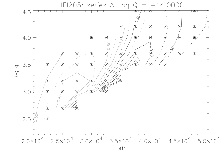
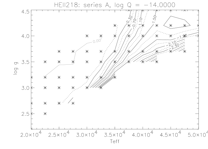
Figure 2: Iso-contours of equivalent widths for Hei and Heii lines using a model-grid with values for $T_{\rm eff}$ and $\log g$ as indicated, and negligible wind densities, $\log Q=-14$. Curves in grey color (left-hand side of Hei2.05 iso-contours) indicate net emission. Note that for the optical transition (Hei4471) the absorption increases as function of gravity, whereas for the NIR lines this behaviour is mostly reversed. Asterisks denote the position of the calculated models (see also Puls et al. 2005).

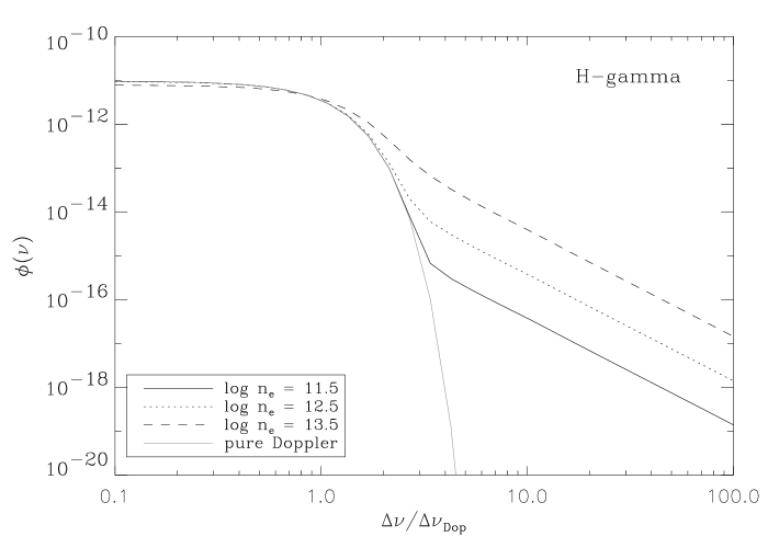
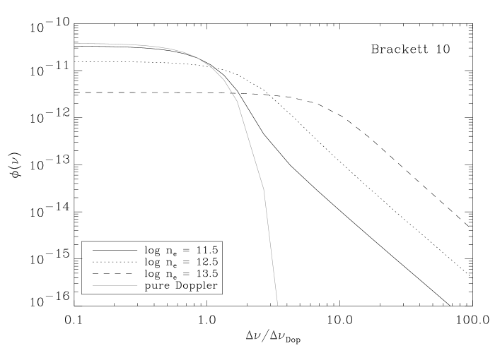
Figure 3: Line broadening profile functions (convolution of Doppler with Stark profiles, in [s^-1]) for H_γ and Br10, as a function of frequency displacement from the line centre in units of thermal Doppler-width. Both profiles have been calculated in Griem approximation, for an electron temperature $T_{\rm e}$ = 40,000 K and three different electron densities typical for the line forming region. The grey line corresponds to a pure Doppler profile. Note that for H_γ the core of the Stark profile is identical with the pure Doppler profile, whereas for Br10 the Stark core is extremely density dependent and coincides with the Doppler profile only at lowest densities (see text).

4.1 Hydrogen and Heii lines: Influence of Stark broadening

The peculiar behaviour of the line cores of the hydrogen Brackett lines and Heii1.69/2.18 can be understood from the reaction of the core of the corresponding Stark-profiles as a function of electron density. Fig. 3 shows the Stark-profiles for H_γ and Br10 as a function of frequency displacement from the line centre in units of thermal Doppler-width, calculated in the Griem approximation. Both profiles have been calculated for typical line-forming parameters, $T_{\rm e}$ = 40,000 K and $\log n_{\rm e}=11.5,12.5$ and 13.5, respectively. The corresponding pure Doppler profile is overplotted (in grey). The decisive point is, that for H_γ, with relatively low upper principal quantum number, the Stark width is not considerably large, and the core of the profile is dominated by Doppler-broadening, independent of electron density. Only in the far wings does the well known dependence on $n_{\rm e}$ become visible. On the other hand, for Br10 the Stark width becomes substantial (being proportional to the fourth power of upper principal quantum number), and even the Stark-core becomes extremely density dependent. Only at lowest densities, the profile coincides with the pure Doppler profile, whereas for larger densities the profile function (and thus the frequential line opacity) decreases with increasing density. In the far cores, finally, the conventional result ($\phi(\nu)$ correlated with $n_{\rm e}$) is recovered. Thus, as a consequence of the dependence of Stark-broadening on density, the line cores of the hydrogen lines with large upper principal quantum number become weaker with increasing gravity. Br_γ (with upper quantum number n=7) is less sensitive to this effect, cf. Fig 1.

In Fig. 4, we demonstrate the different reactions of the Stark profiles on electron density (gravity) by comparing the synthesized emergent profiles of the high- and low-gravity model at $T_{\rm eff}$=40,000 K, as described above. In particular, we compare these profiles with the corresponding profiles calculated with pure Doppler-broadening. For H_γ, the core of the Stark-broadened profile agrees well with the Doppler-broadened one (dashed) in both cases. The major difference is found in the far wings, which become wider and deeper as a function of (electron-) density, thus, being the most useful indicators for the effective gravity. For Br10, on the other hand, the pure Doppler profile is much deeper than the Stark-broadened core, where the differences are more pronounced for the high gravity model. Note particularly that the (absolute) e.w. is larger for the low gravity model (although the high gravity model has more extended wings), since the major part of the profile is dominated by the core which is deeper for lower gravities!

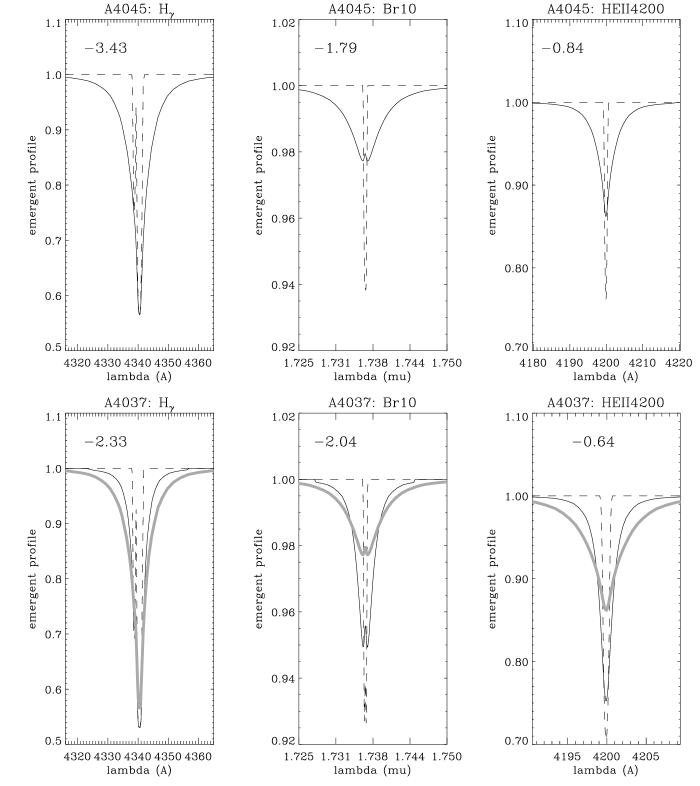
Figure 4: Influence of Stark-broadening for lines with low- and high-lying upper level as a function of gravity. Upper level, solid lines: Synthetic spectra of H_γ, Br10 and Heii4200 (n=4 $\rightarrow$11) for an atmospheric model with $T_{\rm eff}$= 40,000 K, $\log g$=4.5 and $\log Q=-14$ (cf. dashed lines in Fig. 1). Overplotted (dashed) are the corresponding profiles with pure Doppler-broadening. Lower panel: As the upper panel, but for an atmosphere with $\log g$=3.7 (solid lines in Fig. 1). For comparison, the results for the Stark-broadened profiles from the upper panel are overplotted in grey. Note the similarity in effects between Br10 and Heii4200.

Actually, the same effect is already visible in the optical, namely for the prominent Heii lines at 4200Å (transition 4-11) and 4541Å (transition 4-9, not shown here). The increase in absolute e.w. as a function of gravity is solely due to the wings. In accordance with Br10/Br11, however, the cores of the lines become shallower with increasing gravity, not because of an effect of less absorbers, but because of less frequential opacity due to a strongly decreased broadening function.

Let us allude to an interesting by-product of our investigation. A comparison of our synthetic NIR profiles with the observations will show that in a number of cases the observed Br10/Br11 profiles cannot be fitted in parallel. In this case the line formation is well understood and the profiles from cmfgen are identical (note that also the optical hydrogen lines agree well, see Repolust et al. 2004), giving us confidence that our occupation numbers are reasonable and that the obvious differences are due to inadequate broadening functions.

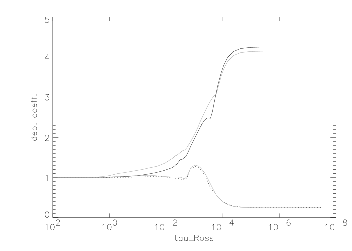
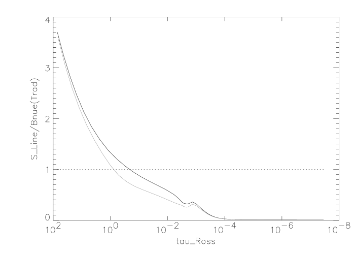
Figure 5: Left panel: NLTE-departure coefficients for the lower (solid) and upper (dotted) levels of Hei1.70 for a model with $T_{\rm eff}$= 30,000 K, $\log g$=3.4 and negligible wind. Overplotted in grey are the corresponding values for a similar model, but with lower gravity, $\log g$=3.0.
Right panel: As the left panel, but for the corresponding line source functions in units of the emergent continuum at 1.70$\mu$m.

On the other hand, since Heii4200/4541 is affected by almost identical line broadening, we would like to suggest a solution for a long standing problem in the optical spectroscopy of hot stars: It is well known that for a wide range of O-star parameters the theoretical simulations of these lines (by means of both plane-parallel and extended atmospheres) have never been able to reproduce the observations in parallel (e.g., Herrero et al. 2002), where the largest discrepancies have been found in the line cores. The origin of this discrepancy is still unknown. Due to the similarity of this problem to the one shown by Br10/11 and accounting for the similar physics, we suggest that also in this case we suffer from an insufficient description of presently available broadening functions (which are described within the VCS-approach, see Schöning & Butler 1989). Thus, a re-investigation of line broadening for transitions with high lying upper levels seems to be urgently required.

In summary, due to their tight coupling with electron density, the cores of Br10/11 and Heii1.69/2.18 are excellent indicators of gravity, where deeper cores indicate lower gravities (if the (projected) rotational velocities are similar).

4.2 Hei lines: Influence of NLTE effects

The peculiar behaviour of the hydrogenic lines could be traced down to the influence of the profile-functions, whereas the formation of most of the NIR Hei lines is dominated by NLTE-effects. As has been extensively discussed by Mihalas (1978), Kudritzki (1979), Najarro et al. (1998), Przybilla & Butler (2004) and Lenorzer et al. (2004), the low value of $h\nu/kT$ leads to the fact that even small departures from LTE become substantially amplified in the IR (in contrast to the situation in the UV and optical). A typical example is given by the behaviour of Hei1.70 at temperatures below $T_{\rm eff}$$\approx$ 35,000 K, cf. Fig. 2 (note, that cmfgen gives identical predictions). Again, this line becomes stronger for lower gravity, in contrast to the well known behaviour of optical lines (compare with the Hei4471 iso-contours).

Fig. 5 gives a first explanation, by means of two atmospheric models with $T_{\rm eff}$=30,000 K, $\log g$=3.4 and 3.0, respectively, and (almost) no wind. The departure coefficient of the upper level, $b_{u}$, of this transition ($4d$ ${}^{3}{\rm D}$) is independent of gravity and has, in the line forming region, a value of roughly unity (strong coupling to the Heii ground-state). The lower level of this transition ($3p$ ${}^{3}{\rm P}^{\rm o}$) is quite sensitive to the different densities, i.e., being stronger overpopulated in the low-gravity model. Consequently, the line source function, being roughly proportional to $b_{u}/b_{l}$, is considerably lower throughout the photosphere (right panel of Fig. 5), and thus the profile is deeper, even if the formation depth is reached at larger values of $\tau_{\rm Ross}$.

The reason for this stronger overpopulation at lower $\log g$-values is explained by considering the most important processes which populate the $3p$-level. First, the influence of collisions is larger at higher densities, which drives the departure coefficient into LTE. Second, the level is strongly coupled to the triplet “ground state” (i.e., the lowest meta-stable state) which, in the photosphere, is overpopulated as an inverse function of the predominant density. The overpopulation (with the consequence of over-populating the $3p$-level) is triggered by the strength of the corresponding ionizing fluxes. These are located in the near UV (roughly at 2,600 Å) and are larger for high gravity models than for low gravity ones. This is because the stronger Lyman-jump and the stronger EUV flux-blocking (higher densities $\rightarrow$ lower metal ionization stages $\rightarrow$ more lines) have to be compensated for on the red side of the flux-maximum to achieve flux conservation.

If the ionization/recombination rates are dominating, the (photospheric) departure coefficients inversely scale with the flux at the corresponding edge (for similar electron temperatures, cf. Mihalas 1978), and for higher gravities we obtain lower departure coefficients (more ionization) than for lower gravities. Thus, the increase of the Hei1.70 line flux with gravity is a final consequence of the different near UV radiation temperatures as a function of gravity.

One might wonder why the strength of Hei4471 is “well” behaved, since this line has the same upper level as Hei1.70, and the lower level ($2p$ ${}^{3}P^{o}$) is strongly coupled to the triplet ground-state as well. Actually, a simple simulation shows that for this transition the same effect as for the Hei1.70 line would be present if the transition were situated in the IR. Only because the transition is located in the optical ($h\nu/kT\gg 1$), the corresponding source functions are much less dependent on gravity (the non-linear response discussed above is largely suppressed). The profiles react almost only on the opacity, which is lower for lower gravity due to the lower number of available Hei ions.

In summary, the Hei line formation in the optical is primarily controlled by different formation regions, since the source functions do not strongly depend on gravity, whereas in the IR the deviations from LTE become decisive. In particular, the influence of considerably different source-functions is stronger than the different formation depths, where these source functions are larger for high-gravity models due to a less overpopulated lower level.

With respect to the singlet transitions (Hei2.05, reacting inversely to the red component of Hei2.11), we refer the reader to the discussion by Najarro et al. (1994) and Lenorzer et al. (2004). But we would like to mention that for a large range of parameters Hei2.05 reacts similar to the way described above, simply because the ionization/recombination rates (over-)populating the lower level ($2s$ ${}^{1}{\rm S}$, again a meta-stable level, located at roughly 3,100 Å) remain the decisive ingredients controlling the corresponding source functions.

Although the basic reaction of Hei2.05 on gravity is readily understood from this argument, we like to point out the following (cf. Najarro et al. 1994). For most of the objects considered here, the upper level of this transition ($2p$ ${}^{1}{\rm P}^{\rm o}$) is populated by the Hei EUV resonance line at 584 Å and other resonance lines (subsequently decaying to this level). Thus, it strongly depends on a correct description of line-blocking in this wavelength range, particularly on lines overlapping with the resonance transitions. Moreover, any effect modifying the EUV will have a large impact on Hei2.05, e.g., wind clumping, if present close to the photosphere. This makes the line generally risky for classification purposes and the determination of $T_{\rm eff}$ in those stars where Heii is no longer present (cf.  Sect. 6.1).

5 Comparison with results by Lenorzer et al.

As already mentioned, Lenorzer et al. (2004) recently presented a first calibration of the spectral properties of normal OB stars using near infrared lines. The analysis was based on a grid of 30 line-blanketed unified atmospheres computed with cmfgen. They presented 10 models per luminosity class I, III, and V, where wind-properties according to the predictions by Vink et al. (2000) have been used, and $T_{\rm eff}$ ranges from 24,000 K up to 49,000 K (cf. Fig. 7). Emphasis was put on the behaviour of the equivalent widths of the 20 strongest lines of H and He in the J, H, K and L band. For detailed information on procedure and results see Lenorzer et al. (2004). In order to check our results obtained by means of fastwind, we have calculated models with identical parameters and synthesized the same set of NIR lines (see also Puls et al. 2005). Note that cmfgen uses a constant photospheric scale height (in contrast to fastwind), so that the photospheric density structures are somewhat different, particularly for low gravity models where the influence of the photospheric line pressure becomes decisive.

Since Lenorzer et al. calculated their hydrogenic profiles with the erroneous broadening functions provided by Lemke (1997), the H and K band profiles have been recalculated by means of the Griem approximation by one of us (R.M.). The differences in the equivalent widths for the dwarf grid are shown in Fig. 6. In all cases the equivalent widths became larger, mainly because of increased line wings, and the most significant changes occurred for Br11 at lower temperatures. Note, however, that also Br_γ has become stronger throughout the complete grid.

Figure 6: Comparison of equivalent widths (defined here in the conventional way) for NIR hydrogen lines of O-type dwarfs (Lenorzer et al. 2004) using the (erroneous) broadening functions by Lemke (1997) with results using broadening functions in the Griem approximation (dashed). Squares, circles and triangles correspond to Br11, Br10 and Br_γ, respectively. Note that in all cases the equivalent width becomes larger and that the most significant differences occur for Br11 at lower temperatures.

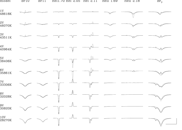
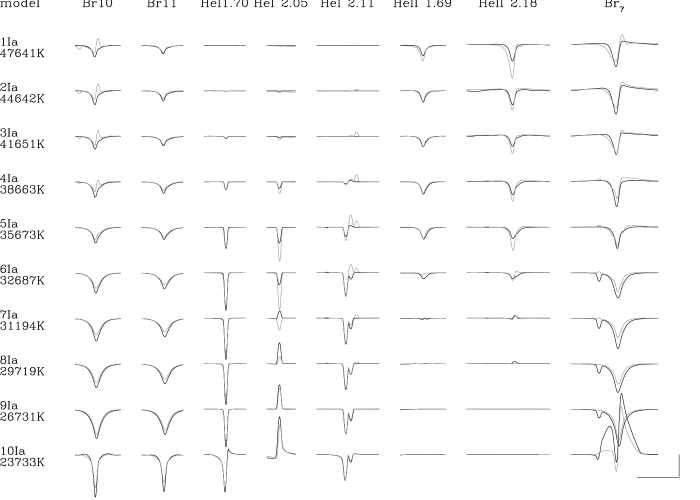
Figure 7: Comparison of synthetic NIR lines for the grid of O-type dwarfs (upper panel) and supergiants (lower panel) described by Lenorzer et al. (2004), as calculated by fastwind and cmfgen (in grey). For hydrogen and Heii, the results reported by Lenorzer et al. have been recalculated using the Griem approximation. The horizontal and vertical lines in the bottom right corner indicate the scale used and correspond to 0.01$\mu$m in wavelength and 0.1 in units of the continuum, respectively. To simplify the comparison, the synthetic profiles have been convolved with a rotational profile corresponding to $v\sin i$ = 80 km s^-1and degraded to a typical resolution of 10,000.

In Fig. 7 we now compare the detailed profiles of the strategic lines located in the H and K band of the present investigation (results from cmfgen in grey). The agreement between the results for the (almost purely photospheric) lines in the H band (Br10/11, Hei1.70 and Heii1.69) is nearly perfect. The only differences occur in the cores of Br10, where cmfgen predicts some emission for hotter objects, and some marginal differences in the far wings of the supergiants, which we attribute to the somewhat different density stratification in the photosphere. Additionally, cmfgen predicts slightly stronger Heii1.69 lines for the hottest objects (models “1V” and “1Ia”) and for the supergiant model “6Ia”.

Concerning the K band, the comparison is also rather satisfactory, except for Hei2.05 at intermediate spectral type (see below). Concerning Br_γ, the dwarf models give rather similar results, with the exception of intermediate spectral types, where fastwind produces some central emission. We have convinced ourselves that this prediction is very stable (and not depending on any temperature inversion), resulting from some intermediate layers where the population of the hydrogen levels is similar to the nebular case. Here the departure coefficients of the individual levels increase as a function of quantum number. In such a situation, a central emission owing to a strong source function is inevitable. For the supergiants, the major differences regard, again, the line cores, with cmfgen predicting more refilling.

Somewhat larger differences are found for Heii2.18, again (cf. Heii1.69) for the hottest models where cmfgen predicts significantly more absorption.

Concerning Hei, the situation for the triplet line (blue component of Hei2.11) is as perfect as for Hei1.70. The differences for the Hei (triplet) component located at the blue of Br_γ are quite interesting. cmfgen predicts an emission for hot stars but “nothing” for cooler objects, whereas fastwind predicts a rather strong absorption at cooler temperatures. To our present knowledge, this is the only discrepancy we have found so far (including the optical range) for a triplet line.

The only important discrepancies concern the Hei singlets (Hei2.05 and the red component of Hei2.11) of the supergiant and dwarf models in the range between models 5 to 7. Starting from the hotter side, cmfgen predicts strong absorption, which abruptly switches into emission at models no. 7, whereas fastwind predicts a smooth transition from strong absorption at model 4 to strong emission at model 8. Reassuring is the fact that at least the inverse behaviour between Hei2.05 and Hei2.11(red) (as discussed in Najarro et al. 1994 and Lenorzer et al. 2004) is always present.

Analogous comparisons performed in the optical (Puls et al. 2005) have revealed that the strongest discrepancies are found in the same range of spectral types. The triplets agree perfectly, whereas the singlets disagree, because they are predicted to be much shallower by cmfgen than the ones resulting from fastwind. Again, the transition from shallow to deep profiles (at late spectral type) occurs abruptly in cmfgen.

Puls et al. (2005) have discussed a number of possibilities which might be responsible for the obvious discrepancy, but at present the situation remains unclear. One might speculate that this difference is due to subtle differences in the EUV, affecting the Hei resonance lines and thus a number of singlet states, as outlined in the previous section. We will, of course, continue in our effort to clarify this inconsistency.

In addition to the detailed comparison performed in the H and K band, we have also compared the resulting e.w.’s of some other important lines in the J and L band. Most important is the comparison for Br_α, which is a primary indicator of mass-loss, as already discussed in Lenorzer et al. (2004). Fig. 8 compares the corresponding e.w.’s, as a function of “equivalent width invariant” $Q^{\prime}$ (see Lenorzer et al.). Generally, the comparison is satisfactory, and particularly the differences at large mass-loss rates are not worrying, since in this range the net-emission reacts strongly on small changes in ${\dot{M}}$. Real differences are found only for the weakest winds, probably related to “uncorrected” broadening functions used by Lenorzer et al.

As we have found for Heii2.18, also the differences for the other Heii lines are significant. Note that we can only compare the e.w.’s and that the broadening as calculated by Lenorzer et al. suffers from erroneous line broadening. For Heii5-7 the behaviour compared to Lenorzer et al. (2004) is the same, but our lines are twice as strong in absorption in the case of giants and dwarfs. For the supergiants we obtain the strongest absorption at 36 kK, in contrast to 42 kK in the comparison models. The only difference found for Heii6-11 concerns the behaviour of supergiant and dwarf line trends. The supergiants in the comparison models show stronger absorption lines than the dwarfs, whereas in our case the situation is reversed.

At high $T_{\rm eff}$, the models for Heii7-13 display a monotonic behaviour with the hottest models showing the strongest absorption. Our hottest models display weaker absorption profiles (as was found in the detailed comparison of Heii1.69 (7-12)), partly due to emission in the line cores. Finally, our emission lines obtained for Heii6-7 are twice as strong in the case of supergiants and giants compared to Lenorzer et al. (2004).

In summary we conclude that at least from a theoretical point of view, all H/K band lines synthesized by fastwind can be trusted, except for Hei2.05 at intermediate spectral type and maybe Heii2.18, where certain discrepancies are found in comparison with cmfgen, mostly at hottest temperatures. Concerning the discrepancies of Heii in other bands, we have to clarify the influence of correct broadening functions, whereas for the Hei singlet problem work is already in progress.

Figure 8: Equivalent width of Br_α as a function of equivalent width invariant Q’ = $\frac{\dot{M}}{R_{\star}^{1.5}\,T_{\rm eff}^{2}\,v_{\infty}}$ (see Lenorzer et al. 2004). The dwarf, giant and supergiant models are denoted by squares, triangles and crosses, respectively. Corresponding values from Lenorzer et al. (2004, their Fig. 7) are given by the end-points of the vertical lines (see text).

6 Analysis

6.1 General remarks

It might be questioned to what extent all decisive stellar and wind parameters can be obtained from a lone IR-analysis in the H and K band. In view of the available number of strategic lines, however, in most cases we are able to obtain the full parameter set, except for

1. the terminal velocity, which in most cases cannot be derived from the optical either, and has been taken from UV-measurements. For our analysis, we have used the values given in the publications corresponding to sample I to III. The terminal velocities of sample IV have been adopted from Howarth et al. (1997). If no information is (or will be) present, calibrations of $v_{\rm\infty}$ as a function of spectral type have to be used, e.g., Kudritzki & Puls (2000).

2. the stellar radius, which can be inferred from M_v and the theoretical fluxes (Kudritzki 1980), and has been taken from the optical analyses in the present work. In future investigations when no optical data will be available, a similar strategy exploiting infrared colors can certainly be established.

In particular, Br10 and Br11 give clues on the gravity (if $T_{\rm eff}$ is known), Hei and Heii define temperature and helium content, and Br_γ can serve as an ${\dot{M}}$ indicator, at least in principle. In those cases, where only one ionization stage of helium is visible, the determination of $Y_{\rm He}$ becomes problematic, and also the uncertainty for $T_{\rm eff}$ increases (see below). Due to the high quality of our spectra, however, both Heii lines are visible for most spectral types.

Only for the coolest objects Heii vanishes, which occurs for spectral types later than O9 for dwarfs, about B0 for giants, and again B0 for supergiants (cf. Figs. 9 to 11). In those cases it still should be possible to derive (somewhat more inaccurate) estimates for $T_{\rm eff}$, at least if some guess for $Y_{\rm He}$ is present. This possibility is due to the behaviour of Hei1.70 vs. Hei2.05 (Fig. 2), since the former line is almost only dependent on $\log g$, whereas the latter depends strongly on $T_{\rm eff}$ (with all the caveats given earlier on). Unfortunately, the data for Hei2.05 are not of sufficient quality (except for HD 190864 and $\tau$ Sco, where the latter just lies in the critical domain) that we could exploit this behaviour only once and had to refrain from an analysis of the remaining coolest objects (four in total).

Because of the independence of Hei1.70 on $T_{\rm eff}$ and the fact that Br10/11 can always be fitted for certain combinations of $T_{\rm eff}$/$\log g$, a perfect fit in combination with completely erroneous parameters would result if Hei2.05 had to be discarded. This is indicated in Fig. 11 for HD 14134, being a B3Ia supergiant (with $T_{\rm eff}$ roughly at 18,000 K, see Kudritzki et al. 1999), which could be fitted with $T_{\rm eff}$ = 25,000 K. If, on the other hand, Hei2.05 had been available, the appropriate parameters should have been obtained, at least when the helium content could have been guessed. Such a guess of the helium abundance should always be possible for objects we are eventually aiming at in our project (cf. Sect. 1), i.e., for very young, un-evolved stars with unprocessed helium.

Micro-turbulence.

In agreement with the findings by Repolust et al. (2004), we have adopted a micro-turbulence of $v_{\rm turb}$ = 10km s^-1 for all stars with spectral type O7 or later regardless of their luminosity class, whereas for hotter O-type stars the micro-turbulent velocity has almost no effect on the analysis and we have neglected it. At spectral type O6.5, our IR-analysis of HD 190864 (O6.5 III) indicated that a micro-turbulence is still needed, whereas from O7 onwards $v_{\rm turb}$ did not play any role, e.g., for HD 192639 (O7 Ib). Since the former and the latter stars have $T_{\rm eff}$ = 37 and 35 kK, respectively, we conclude that at roughly $T_{\rm eff}$ = 36 kK the influence of $v_{\rm turb}$ on the H/He lines is vanishing, in agreement with our previous findings from the optical.

Rotational velocities.

For the (projected) rotational velocities, we have, as a first guess, used the values provided by Repolust et al. (2004), Herrero et al. (2000, 2002) and Howarth et al. (1997) for sample I, II and III/IV, respectively. In our spirit to rely on IR data alone, we have subsequently inferred the rotational velocity from the (narrow) He lines, with most emphasis on Hei. Concerning sample I, the results from our IR-analysis are consistent with the velocities derived from the optical, except for HD 190864 and HD 192639, where the profiles indicated slightly lower values (10% and 20%, respectively), which have been used instead of the “original” ones.

For sample II stars, in 3 out of 5 cases the “optical” values derived by Herrero et al. (2000, 2002) were inconsistent with our IR-data. In particular, for HD 5689 we found a velocity of 220 km s^-1 (instead of 250 km s^-1), for HD 15570 a velocity of 120 km s^-1 (instead of 105 km s^-1) and for Cyg OB2#7 our analysis produced the largest differences, namely $V_{\rm r}$ sin $i$ = 145 km s^-1, compared to a value of 105 km s^-1provided by Herrero et al. (2002) (30% difference!).

The values taken from Howarth et al. (1997) for the remaining sample III/IV objects, finally, agree fairly well with our IR data, and are also consistent with the values derived by Kudritzki et al. (1999) in their analysis of sample III objects.

Let us finally mention that in those cases when Br_γ does not show emission wings, a statement concerning the velocity field parameter, $\beta$, is not possible, as is true for the optical analysis. In order to allow for a meaningful comparison with respect to optical determinations of ${\dot{M}}$, we have used the corresponding values derived or adopted from the optical. In future analyses, of course, this possibility will no longer be present, and we have to rely on our accumulated knowledge, i.e., we will have to adopt “reasonable” values for $\beta$, with all related problems concerning the accuracy of ${\dot{M}}$ (cf. Puls et al. 1996; Markova et al. 2004).

6.2 Fitting strategy and line trends

In order to obtain reliable fits, we applied the following strategy. At first, we searched for a coarse determination of the relevant sub-volume in parameter space by comparing the observed profiles with our large grid of synthetic profiles as described by Puls et al. (2005), which has a typical resolution of 2,500 K in $T_{\rm eff}$, 0.3 in $\log g$, and 0.25 in $\log Q$. A subsequent fine fit is obtained by modifying the parameters by hand (using the “actual” values for $R_{\ast}$ and $v_{\rm\infty}$ to obtain information on ${\dot{M}}$ additionally to $\log Q$), where typically 10 trials are enough to provide a best compromise. In those cases, where at present no information about $R_{\ast}$ is available (which concerns the three objects presented in Table 2), “only” $\log Q$ can be derived. For the actual fits of these three objects we have, of course, used prototypical parameters for $R_{\ast}$ and $v_{\rm\infty}$. Further discussion of related uncertainties is given in Sect. 7.

Most weight has been given to the fits of the He lines (which are rather uncontaminated from errors in both broadening functions and reduction of the observed material) followed by the photospheric hydrogen lines, Br10/11, which sometimes strongly suffer from both defects. Least weight has been given to Br_γ, because of the number of problems inherent to this line, as recently described by Lenorzer et al. (2004) and independently found by Jokuthy (2002). Particularly, the synthetic profiles for larger wind densities, predicted by both fastwind and cmfgen, are of P Cygni type, whereas the observations show an almost pure emission profile. Moreover, from a comparison of equivalent widths, it has turned out that in a lot of cases the predicted e.w. is much larger than the observed one, which would indicate that the models underestimate the wind-emission (remember, that Br_γ forms inside the H_α sphere). Often, however, this larger e.w. is due to the predicted P Cygni absorption component which is missing in the observations, and we tried to concentrate on the Br_γ line wings in our fits ignoring any discrepancy concerning the predicted P Cygni troughs. If the synthetic lines actually predicted too few wind emission, this problem would become severe for lines where pure absorption lines are observed, and should lead to an overestimate of ${\dot{M}}$. We will come back to this point in the discussion of our analysis.

Another important point to make concerns the Hei $\lambda$2.11 line (comprising the Hei triplet $\lambda$2.1120 and the Hei singlet $\lambda$2.1132). Close to its central frequency, a broad emission feature can be seen (at $\lambda$2.115) in the spectra of hot stars. This line can either be identified as Niii (n = 7 $\rightarrow$8) or as Ciii (n = 7 $\rightarrow$8) or maybe both (Hanson et al. 1996; Najarro et al. 1997a, 2004). This feature is seen in stars of all luminosity classes, for stars hotter than and including spectral type O8 in the case of dwarfs and giants and O9 in the case of supergiants (though its designation is somewhat unclear, as Hei2.11 resembles a P Cygni profile in late-O supergiants, possibly mimicking this feature). Since our present version of fastwind synthesizes “only” H/He lines and their analysis is the scope of the present paper, we are not able to fit this feature, but have to consider the fact that this feature significantly contaminates Hei2.11.

Due to the well-resolved spectra, the two Hei lines overlapping with Br_γ as mentioned in Sect. 2, i.e., the Hei triplet $\lambda$2.1607 and the Hei singlet $\lambda$2.1617, are also visible in certain domains. For supergiants later than O5, Hei2.1607 begins to appear in the blue wings of Br_γ, and in two stars, HD 30614 and HD 37128, the Hei2.1617 singlet seems to be present, even if difficult to see. In the giant spectra, Hei2.1607 can be seen from spectral type O9 onwards, and in the dwarf spectra this line appears in spectral types later than O8.

The strength of the Brackett lines in supergiants (Fig. 11) shows a smooth behaviour as a function of spectral type, apart from certain fluctuations such as blends in the late O- and early B-type stars. As one moves from early B-type to mid O-type (i.e., O5), the Br_γ absorption weakens, and from mid to the earliest O-types the line profiles switch into emission, where the emission at the blue wings of Br_γ is much more pronounced (except for HD 15570), presumably due to the overlapping Heii blend.

As for the photospheric Br10/11 lines, we can see that these absorption profiles show an extremely continuous behaviour, being rather weak for early O-type stars and increasing in strength towards early B-types. Hence, the cooler supergiants show the most prominent and sharpest absorption features. The emission features visible at the blue side of Br10 in the hottest supergiants are due to an unidentified feature.

Fig. 11 shows that the observed Br10/11 profiles are mostly well reproduced by the theoretical predictions, although at hotter temperatures certain inconsistencies arise, particularly with respect to the line cores. Most interestingly, in a number of cases we could not fit both profiles in parallel, and typically Br11 is then of better quality. Since we have convinced ourselves that the differences most probably are not exclusively due to reduction problems, we repeat our hypothesis that the broadening functions are somewhat erroneous, cf. Sect.  4.1. Again, for the theoretical profiles for Br_γ, we would like to mention that for emission lines the wings are fairly well reproduced in contrast to the line cores.

The Hei1.70 line shows a very smooth behaviour, being absent in the hottest and most luminous star, Cyg OB2 $\#$7, and successively increasing towards late O-type and early B-type stars. This also applies to the sharpness of the profiles. As has been stressed earlier on, Heii1.69 and Heii2.18 vanish in supergiants of spectral type B0 (being still detectable for $\alpha$ Cam, O9.5Ia)

The situation is similar in the case of giants (Fig. 10) and dwarfs (Fig. 9). All hydrogen and Hei lines show the systematic variations expected, namely, an increase in strength from early O-types to early B-types. The model predictions do agree well with the observed profiles, again, except for certain discrepancies between Br10 vs. Br 11. Since Br_γ remains in absorption throughout the entire spectral range, it can be reasonably fitted in most cases (whether at the “correct” value, will be clarified in Sect. 8). Particularly, the Heii profiles give almost perfect fits except for very few outliers, and vanish at 09 for dwarfs and about B0 for giants.

Figure 9: Line fits for hot dwarfs with spectral types ranging from O3 to O7 (upper panel) and cool dwarfs with spectral types ranging from O8 to B2 (lower panel). The lowermost object (HD 36166, B2V) has not been analyzed due to missing Heii and Hei2.05 (see text). The horizontal and vertical lines in the bottom right corner indicate the scale used and correspond to 0.01 microns in wavelength and 0.10 in units of the continuum, respectively.

6.3 Comments on the individual objects

In the following, we will comment on the fits for the individual objects where necessary. Further information on the objects can be found in the corresponding publications concerning the optical analyses, see Tab. 1. A summary of all derived values can be found in Tables 2 and 4.

6.3.1 Dwarfs

Figure 10: As Fig. 9, but for giants with spectral types ranging from O5 to B9. Concerning HD 15558 (only H band available), see text.

HD 64568.

The fit quality of the lines is generally good except for Br_γ. The theoretical profile displays a central emission which is more due to an overpopulated upper level than due to wind effects (cf. Sect. 5) and, thus, cannot be removed by adopting a lower ${\dot{M}}$. Moreover, the theoretical Heii line would become too strong if a lower ${\dot{M}}$ were used. Insofar, the present fits display the best compromise. Since no radius information is available, only the optical depth invariant $\log Q$ is presented.

HD 46223 and HD 46150.

For both objects, the fit quality is satisfactory, except for the Heii lines (particularly in HD 46150) and Br_γ. The former lines are predicted to be too strong and for the latter there is, again, too much central emission present. It is, however, not possible to reduce the temperature in order to fit the Heii line, since this would adversely affect Hei. A further reduction of $Y_{\rm He}$ (adopted here to be “solar”, i.e., 0.1) is implausible, so that the presented line fits reveal the best fit quality possible. For HD 46223 we can derive only the optical depth invariant $\log Q$ due to missing radius information.

HD 15629.

The fit quality for the He lines is very good, and we confirm the helium deficiency to be $Y_{\rm He}$ = 0.08 as determined in the optical, see Repolust et al. (2004). Br_γ, again, suffers from too much central emission, and the cores of Br10/11 are much narrower than predicted (at least partly, as some of the narrowness might be due to reduction problems). The mass-loss rate is moderate with a value of $\dot{M}\approx$ 1.3 $\cdot 10^{-6}{\rm M_{\odot}/yr}$ which represents the same value as determined in the optical, whereas $\log g$ is found to be larger by 0.1 dex.

HD 5689.

Again, moderate mismatches for the H lines are found, whereas the He lines provide a good fit. Br_γ does not show a central emission anymore, but the theoretical profile seems to be too broad. The same problem (very steep increase on the blue side, almost perfect fit on the red side) seems to be present also in HD 217086 (and, to a lesser extent, in HD 203064 and HD 191423), and we attribute some of this disagreement to reduction errors, although an underestimate of the Heii blend (which is in emission in this parameter range) might be possible as well. Since all four stars are very fast rotators, effects from differential rotation in combination with a non-spherical wind (cf. Puls et al. 1996; Repolust et al. 2004 and references therein) cannot be excluded, see below.

In the case of Br10/11, on the other hand, problems in the broadening functions might explain the disagreement, as already discussed. Finally, the absorption trough of the theoretical profile for Hei2.11 seems to be too strong, but might be contaminated by the bluewards Niii/Ciii complex.

HD 217086.

A very similar fit quality as found for HD 5689 has been obtained for this star, although Br10/11 are now in better agreement. The parameters determined are comparable to the ones obtained from the optical, including the overabundance of He ($Y_{\rm He}$ = 0.15). An upper limit for the mass-loss rate has been derived, which is less than half the value obtained from the optical.

HD 13268.

The theoretical prediction reproduces the observation quite well, especially in the case of Hei1.70 and both Heii lines. As for the hydrogen lines, the two photospheric lines Br10 and Br11 show too much absorption in the line cores, whereas Hei2.11 shows the same trend as already discussed for HD 5689. The fit quality for Br_γ, however, is much better, and even the Hei2.1607 (triplet) blend is reasonably reproduced, although slightly too strong. For the mass-loss rate only an upper limit of 0.17 $\cdot 10^{-6}{\rm M_{\odot}/yr}$ can be given, for an adopted value of $\beta$ = 0.80. The enhanced helium abundance $Y_{\rm He}$ = 0.25, as found in the optical, could be confirmed, giving the best compromise regarding all He lines.

HD 149757 and HD 37468.

The very good fit quality makes further comments unnecessary.

HD 149438.

$\tau$ Sco is probably one of the most interesting stars of the sample analyzed, since it is a very slow rotator and all features become visible at the obtained resolution. Although only the K band observation is available, it can be seen that we obtain a very good fit quality for all H and He lines present (Heii is absent at these temperatures). As discussed before, in those cases where only one ionization stage of helium is visible, the determination of $Y_{\rm He}$ becomes problematic, and also the uncertainty for $T_{\rm eff}$ increases. Since in the case of $\tau$ Sco we could make use of the Hei2.05 line, we could still determine the effective temperature (resulting in a similar value as in the optical), on the basis of an adopted value $Y_{\rm He}$ = 0.1. Also the mass-loss rate is well constrained from the resolved central emission feature in Br_γ, having a value of 0.02 $\cdot 10^{-6}{\rm M_{\odot}/yr}$. From a similar investigation by Przybilla & Butler (2004), exploiting the central emissions of Pf_γ, Pf_β and Br_α as well, they derived a value of 0.009 $\cdot 10^{-6}{\rm M_{\odot}/yr}$ (factor two lower) as a compromise, but have adopted a different velocity-field exponent ($\beta=2.4$ instead of $\beta=1.0$ used here) and utilized the “canonical” value for $\log g$ = 4.25 which fits H_γ. In our case, however, and in the spirit to rely on a lone IR analysis, we preferred a lower value, $\log g$ = 4.0, since in this case the emission feature is better reproduced (much narrower) than for a higher gravity, whereas the differences in Hei2.05 (and concerning the line wings of Br_γ!) are almost negligible. If we have had the information on Br10/11, this dichotomy could have been solved.

Having finished our investigation, one of us (R.M.) has analyzed the optical spectrum of $\tau$ Sco, also by means of fastwind. Details will be published elsewhere (Mokiem et al. 2005). Most interestingly, he obtained perfect line fits, at parameters $T_{\rm eff}$= 31,900 K, $\log g$ = 4.15, $Y_{\rm He}$ = 0.12 and ${\dot{M}}$ = 0.02 … 0.06 $\cdot 10^{-6}{\rm M_{\odot}/yr}$ (for velocity exponents $\beta$ = 2.4 … 0.8, respectively). We like to stress that this analysis has not been biased by our present results from the IR, since it was performed by an “automatic” line fitting procedure based on a genetic algorithm.

HD 36166.

This object has not been analyzed, due to missing Heii and Hei2.05 lines.

6.3.2 Giants

HD 15558.

Also for this star, only the K band observation is available, and because of the high temperature and rather large ${\dot{M}}$ no independent information concerning $T_{\rm eff}$ and $\log g$ can be derived. Thus, we adopted the effective temperature at its “optical” value, $T_{\rm eff}$ = 41,000 K. With this value, a simultaneous “fit” of $\log g$, $Y_{\rm He}$ and ${\dot{M}}$ resulted in the synthetic spectrum displayed. ${\dot{M}}$ was constrained by the wings of Br_γ, and $Y_{\rm He}$ = 0.08 derived on the basis that at this value Heii is still somewhat too strong. $\log g$ is rather badly defined, since a variation by $\pm 0.2$ dex gives only small differences in all three observed lines. In conclusion, the fit obtained allows to reliably constrain the mass-loss rate alone, and this only if the temperature actually has the adopted value. Note, however, that a (much) lower value is excluded since the predicted Heii2.18 line would become too weak (cf. Fig 2, lower right panel).

HD 190864.

The analysis gives a consistent fit for all lines (including Hei2.05!) except for Br_γ, where the theoretical profile of Br_γ shows too much central emission. The parameters remained almost the same compared to the optical except for the helium abundance, $Y_{\rm He}$, which has been increased from 0.15 to 0.20.

HD 203064 and HD 191423.

The analysis for HD 203064 yields a consistent fit for all lines, except for Hei2.11 which displays a similar problem as described for HD 5689. We recovered the same values for $T_{\rm eff}$ and $\log g$ as in the optical, though the helium abundance had to be doubled and also the mass-loss rate increased by roughly 80%. The theoretical profile of Br_γ for both stars is slightly broader than observed, although the effect is weaker than found for HD 5689 and HD 217086. Note in particular that for both giants H_α turned out to be narrower than predicted, with “emission humps” present on both sides of the absorption trough (Repolust et al. 2004, Fig. 6). Summarizing and considering their extreme rotation velocities ($V_{\rm r}$ sin $i$ being 300 km s^-1and 400 km s^-1for HD 203064 and HD 191423, respectively), our above hypothesis of rotational distortion is the most probable solution for the apparent dilemma in these cases.

Also for all other lines, HD 191423 behaves very similarly to HD 203064, although a better fit quality for Hei2.11 is found, while Hei1.70 has become worse (we aimed for a compromise between both lines).

6.3.3 Supergiants

Figure 11: As Fig. 9, but for hot supergiants of spectral type O3 to O7 (upper panel) and cool supergiants (O9 to B3, lower panel). The three lowermost objects (HD 13854, B1Iab, HD 13866, B2Ib and HD 14134, B3Ia) have not been analyzed. The synthetic profiles overplotted for HD 14134 show a perfect fit for completely wrong parameters ($T_{\rm eff}$= 25,000 K, $\log g$= 2.7), indicating that a spectroscopic H/K band analysis is impossible if Heii and/or Hei2.05 are missing (see text).

Cyg OB2 $\#$7.

This star, being the hottest one in the sample, shows an enormous discrepancy in the Br_γ line, due to the observed central emission, which is not predicted by our simulations. It is the only star in our sample where we find the same problem in Heii2.18, i.e., where the theoretical predictions with respect to its morphology could not be confirmed. In order to determine a fairly reliable mass-loss rate, we have concentrated exclusively on the wings of Br_γ. The parameters derived agree with their values from the optical, except for the helium abundance. The determination of this quantity is problematic due to missing Hei. In contrast to the optical value, $Y_{\rm He}$ = 0.3 (Herrero et al. 2002), our best fit favoured $Y_{\rm He}$ = 0.1, whereas simulations using the optical value have adversely affected the H lines. Moreover, to preserve the good fit quality of Heii1.69, we would have to lower $T_{\rm eff}$ significantly if $Y_{\rm He}$ = 0.3 were the correct value. (Actually, a temperature already lower by 1,500 K compared to the optical has been used to achieve the displayed fit). Interestingly, a re-analysis of Cyg OB2 $\#$7 in the optical performed by one of us (R.M.) resulted in a value just in between, namely $Y_{\rm He}$ = 0.21 (at $T_{\rm eff}$ = 46,000 K). The emission on the blue side of Br10 is due to an unknown feature, as discussed in Sect. 6.2.

HD 66811.

The fit quality is generally good, except for Br_γ, which again shows much more central emission than predicted. The wings, on the other hand, could be well fitted and gave a mass-loss rate of 8.8 $\cdot 10^{-6}{\rm M_{\odot}/yr}$, in agreement with the optical value. Br10 is contaminated by an unknown feature on the blue side, but to a lesser extent than in Cyg OB2 $\#$7.

HD 15570 and HD 14947

show very similar profiles, and could be reasonably well fitted. Note the prominent emission in Br_γ. This could not be matched, so we had to concentrate on the wings. In both cases Heii2.18 gives an additional constraint on ${\dot{M}}$, since at higher values the (theoretical) wings would show too much emission.

Cyg OB2 $\#$8C and Cyg OB2 $\#$8A.

These stars, being of rather similar type and displaying rather similar profiles (with the noticeable difference of Hei1.70, immediately indicating that 8A is somewhat cooler than 8C), have been carefully analyzed in the optical (and, again, re-analyzed by R.M.). From the optical, both stars have significantly different gravities (well constrained from the Balmer line wings), where object 8C with $\log g$ = 3.8 has a rather large gravity for its type, cf. Herrero et al. (2002). The values derived from the IR, on the other hand, are much closer to each other, namely 3.62 and 3.41, respectively. According to the observed shape of the profiles and their corresponding theoretical fits, a higher $\log g$ would lead to severe inconsistencies. Apart from gravity, however, the other parameters derived are comparable to their optical counterparts, including the differences in ${\dot{M}}$, although the fit quality of Br_γ is dissatisfying.

HD 192639.

For this star, we found a reasonable compromise concerning the fit quality of the lines present. We derived a $\log g$ value of 3.3 compared to 3.45 in the optical, because of the wings Br10/11 (note the different degree of inconsistency in the lines cores!) and due to the shape of Heii2.18. With a value of $\log g$ = 3.45 Heii2.18 becomes even narrower, with a more pronounced P-Cygni type profile. The helium abundance was raised to 0.3 (from 0.2 in the optical) in order to fit the Hei and Heii lines appropriately in combination with the derived $T_{\rm eff}$. Also in this case, the observed Br_γ line shows a central emission which could by no means be reproduced. The Hei2.1607 triplet blend showing up in the theoretical prediction is not yet present in the observation.

HD 210809.

Part of the observed discrepancy in Br_γ might be attributed to intrinsic variations in the notoriously variable wind of this star (Markova et al. 2005), though it is also possible that some (though not all) of the mismatch arises from errors in the removal of the Br_γ feature in the telluric standard. Fortunately, the line wings could be fitted fairly well, resulting in a mass-loss rate of 5.80 $\cdot 10^{-6}{\rm M_{\odot}/yr}$ compared to 5.30 $\cdot 10^{-6}{\rm M_{\odot}/yr}$ in the optical. The major difficulty encountered was to fit the Hei and Heii lines simultaneously. In fact, a decrease in $T_{\rm eff}$ leads to an even more pronounced P-Cygni type profile for Heii2.18 for the given mass-loss rate, as was already true for HD 192639. We regard our solution as the best compromise possible, accounting for the fact that by a reduction in $T_{\rm eff}$ we would also increase the apparent dilemma in Br10/11 and the Hei component in Br_γ. The helium abundance was raised by 0.06 to 0.2 in order to find a compromise for the He lines.

HD 30614.

For this star a very good fit quality was obtained making further comments unnecessary.

HD 209975.

The stellar profiles are fairly well reproduced and represent the best compromise possible. All hydrogen features predicted are a little too strong, with some contamination on the blue side of the profiles. The parameters obtained are comparable to the optical ones, except for $\log g$, where we determined a smaller value (0.15 dex).

Table 2: Adopted and derived stellar and wind parameters obtained from spectra in the infrared for sample IV objects not analyzed in the optical. Since no radius information is available, only the optical depth invariant, $\log Q$, can be derived (Eq. 1). $T_{\rm eff}$ in kK, $V_{\rm r}$ sin $i$ in km s^-1. Centrifugal correction ($\rightarrow\log g_{\rm true}$) assuming a typical radius.

Star	Sp.Type	$T_{\rm eff}$	$\log g$	$\log g_{\rm true}$	$Y_{\rm He}$	$V_{\rm r}$ sin $i$	$\log Q$	$\beta$
HD 64568	O3 V((f))	45.0	3.85	3.86	0.10	150	- 13.00	0.90
HD 46223	O4 V((f))	42.0	3.70	3.71	0.10	100	-12.70	0.90
HD 37468	O9.5 V	30.0	4.00	4.00	0.10	80	-14.10	1.00

HD 37128 ($\epsilon$ Ori).

Almost perfect fit. Let us only point out that the derived value for $T_{\rm eff}$ represents an upper limit, since from this star onwards Heii is no longer present and Hei becomes rather insensitive to $T_{\rm eff}$, so that without Hei2.05 further conclusions are almost impossible.

HD 13854 and HD 13866

have not been analyzed, due to missing Heii and Hei2.05.

HD 14134.

As above. The “theoretical” spectrum displayed in Fig 11 shows the insensitivity of the Hei1.70 and Hei2.11 lines to $T_{\rm eff}$ for temperatures below 30,000 K. Although a virtually perfect fit has been obtained, the synthetic model ($T_{\rm eff}$ = 25,000 K, $\log g$ = 2.70) is located far away from realistic values (roughly at $T_{\rm eff}$ = 18,000 K, $\log g$ = 2.20, cf. Kudritzki et al. 1999).

7 The “$\log Q$-approach”

Before we compare our results from the IR with optical data, let us briefly consider those objects where no optical information is available. Tab. 2 summarizes the corresponding parameters which constitute a “by-product” of our investigations. Because of the missing radius information, we quote the corresponding values for the optical depth invariant, $\log Q$, instead of the mass-loss rate ${\dot{M}}$.

Though we will no longer comment on these stars in the following, we would like to point out that all derived parameters appear to be fairly reasonable, except for the gravity of HD 46223, which is rather low for a dwarf of spectral type O4.

It might be questioned how reliable these parameters are, given the fact that, more precisely, $\log Q$ is actually a scaling-quantity for recombination lines formed in the wind. As outlined by Puls et al. (2005), however, this quantity is a suitable compromise concerning the scaling properties of other important physical variables, namely density ($\propto\dot{M}/(R_{\star}^{2}v_{\infty})$) and the optical depth of resonance lines from major ions (scaling via $\dot{M}/(R_{\star}v_{\infty}^{2})$). Thus, it might be used as a general scaling invariant, though only in an average sense. Because of these different scaling properties, it is to be expected that models with identical $\log Q$ but different combinations of $R_{\ast}$, $v_{\rm\infty}$ and ${\dot{M}}$ result in somewhat different profiles, and in the following we will explore the corresponding uncertainties. By this investigation, we will also clarify in how far uncertainties in stellar radii (i.e., distances) and terminal velocities (which will be present in future applications when analyzing the IR alone, cf. Sect. 6.1) might influence the derived parameters, particularly $\log Q$.

Table 3: Different models for $\zeta$ Pup at identical $\log Q=-12.02$. The first entry corresponds to our reference model (for additional parameters, cf. Table 4). For models A to D we have varied $R_{\ast}$, $v_{\rm\infty}$ and ${\dot{M}}$ in such a way as to preserve the optical-depth invariant $Q$ whereas the other parameters remain unchanged. $R_{\ast}$ in $\rm{R_{\odot}}$, $v_{\rm\infty}$ in km s^-1and ${\dot{M}}$ in 10^-6$\rm{M_{\odot}}$/yr (see text and Fig. 12).

Model	$R_{\ast}$	$v_{\rm\infty}$	${\dot{M}}$	$\log Q$
HD 66811	19.4	2250	8.77	-12.02
HD 66811-A	15.0	1900	4.56	-12.02
HD 66811-B	15.0	2550	7.19	-12.02
HD 66811-C	25.0	1900	9.94	-12.02
HD 66811-D	25.0	2550	15.46	-12.02

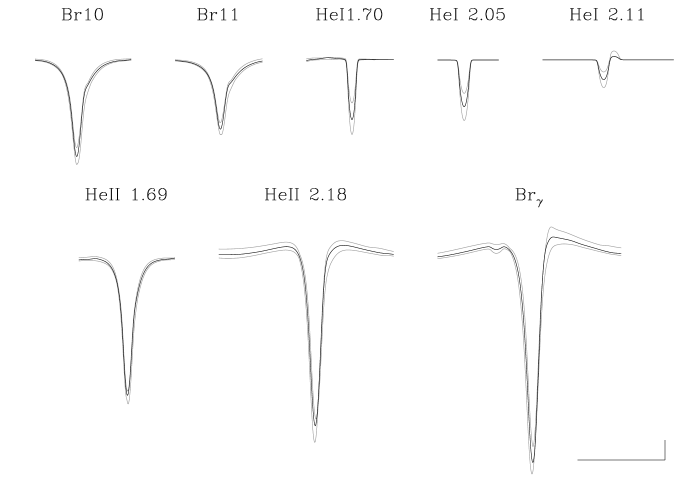
Figure 12: Variation of synthetic IR spectra for different combinations of $R_{\ast}$, $v_{\rm\infty}$ and ${\dot{M}}$ but identical optical depth invariant $Q$. Bold: profiles for our reference model of $\zeta$ Pup. Grey: maximum und minumum profiles resulting from the models A to D of Table 3 and the reference model, see text. The scale in the lower left corner corresponds to 0.01 microns in wavelength and 1% of the continuum, respectively. Note that in almost all cases the maximum/minimum variations are below this value. All original profiles have been convolved with a typical rotational speed of $v\sin i$ = 100 km s^-1.

A first impression of this problem has been given by Puls et al. (2005, Fig. 18) who discussed the variations of the synthetic optical spectrum of $\alpha$ Cam when the stellar radius is modified, while keeping the terminal velocity and $Q$. The differences turned out to be marginal, except for the innermost cores of a variety of lines. H_α (being the prototypical recombination wind line), on the other hand, showed perfect agreement with the original profile.

We have performed a corresponding analysis in the IR, additionally allowing for variations in $v_{\rm\infty}$, by means of our best fitting model for $\zeta$ Pup, cf. Table 4. Our choice was motivated by the fact that this object is one of the few which shows a certain degree of wind-emission in the wings of Br_γ and Heii2.18, thus displaying profiles which have a significant contribution from the wind. We have calculated four additional models, denoted by A to D, where the modified stellar/wind-parameters (constrained by the requirement of preserving $Q$) are displayed in Table 3. In particular, we have varied $R_{\ast}$ = 19.4 $R_{\odot}$ by roughly $\pm$ 25% and $v_{\rm\infty}$ = 2250 km s^-1 by $\pm$ 300 km s^-1, consistent with the typical uncertainties in $R_{\ast}$ and $v_{\rm\infty}$ if taken from calibrations. Within the four models, the mass-loss rates (with a reference value of 8.5 $\cdot 10^{-6}{\rm M_{\odot}/yr}$) range from ${\dot{M}}$ = 4.6 to 15.5 $\cdot 10^{-6}{\rm M_{\odot}/yr}$.

In Fig. 12 we compare the resulting variations of the corresponding profiles with our reference solution from Fig. 11. Since the differences turned out to be rather small, we display, at each frequency point, the minimum and maximum normalized flux value with respect to all five spectra, in order to illustrate the maximum uncertainty due to the various parameter combinations. As it is evident, in almost all cases this maximum uncertainty lies well below $\pm$ 1% of the continuum flux level, at least if $v\sin i$ is not very low. Accounting for the additional noise within the observation, we would have derived almost identical stellar parameters including $\log Q$ (with differences well below the typical errors as discussed in the next section) if a fit by any of the additional models had been performed. Thus, our hypothesis that $\log Q$ can be used as a global scaling invariant is justified indeed.

Table 4: Comparison of stellar and wind parameters in the optical and the near infrared derived using fastwind. $T_{\rm eff}$ in kK, $R_{\ast}$ in $\rm{R_{\odot}}$, ${\dot{M}}$ in 10^-6$\rm{M_{\odot}}$/yr. $\log g$ values are corrected for centrifugal acceleration. If not explicitely indicated, the optical parameters have been taken from Repolust et al. (2004). Note that Cyg OB2 $\#$8A has been recently identified as an O6 I/O5.5 III binary system. In order to compare with previous analyses, we have retained its single star designation as used by Herrero et al. (2002)

. Star Sp.Type $R_{\ast}$ $T_{\rm eff}^{\rm opt}$ $T_{\rm eff}^{\rm ir}$ $\log g^{\rm opt}_{\rm true}$ $\log g^{\rm ir}_{\rm true}$ $Y_{\rm He}^{\rm opt}$ $Y_{\rm He}^{\rm ir}$ ${\dot{M}}^{\rm opt}$ ${\dot{M}}^{\rm ir}$ Cyg OB2 $\#$7¹⁾ O3 If^∗ 14.6 45.5 44.0 3.71 3.71 0.21^a)-0.30 0.10 9.86 10.00 HD 66811 O4 I(n)f 19.4 39.0 39.0 3.59 3.59 0.20 0.17 8.80 8.77 HD 15570²⁾ O4 If+ 22.0 42.0 38.0 3.81 3.51 0.18 0.15 17.8 15.20 Cyg OB2 $\#$8C¹⁾ O5 If 13.3 41.0 39.0 3.81 3.62 0.09 0.10 2.25 2.00 HD 14947 O5 If+ 16.8 37.5 37.5 3.48 3.48 0.20 0.20 8.52 7.46 Cyg OB2 $\#$8A¹⁾ O5.5 I(f) 27.9 38.5 37.0 3.51 3.41 0.10 0.10 13.5 11.50 HD 192639 O7 Ib 18.7 35.0 34.0 3.47 3.32 0.20 0.30 6.32 6.32 HD 210809 O9 Iab 21.2 31.5 32.0 3.12 3.31 0.14 0.20 5.30 5.80 HD 30614 O9.5 Ia 32.5 29.0 29.0 2.99 2.88 0.10 0.20 6.04 6.04 HD 209975 O9.5 Ib 22.9 32.0 31.0 3.22 3.07 0.10 0.10 2.15 3.30 28.5 3.00 0.10 2.40 HD 37128³⁾ B0 Ia 35.0 27.5 29.0^b) 2.95 3.01 0.10 0.10 3.01 5.25 HD 15558 O5 III(f) 18.2 41.0 41.0^c) 3.81 3.81 0.10 0.08 5.58 7.10 HD 190864 O6.5 III 12.3 37.0 36.5 3.57 3.61 0.15 0.20 1.39 0.98 HD 203064 O7.5 III 15.7 34.5 34.5 3.60 3.60 0.10 0.20 1.41 2.58 HD 191423 O9 III 12.9 32.5 32.0 3.60 3.56 0.20 0.20 $\leq$ 0.41 $\leq$ 0.39 HD 46150⁴⁾ O5 V((f)) 13.1 43.0 40.0 3.71 3.71 0.10 0.10 N/A 1.38 HD 15629 O5 V((f)) 12.8 40.5 40.5 3.71 3.81 0.08 0.08 1.28 1.28 HD 5689²⁾ O6 V 7.7 37.0 36.0 3.57 3.66 0.33 0.20 0.16 0.17 HD 217086 O7 Vn 8.6 36.0 36.0 3.72 3.78 0.15 0.15 $\leq$ 0.23 $\leq$ 0.09 HD 13268 ON8 V 10.3 33.0 33.0 3.48 3.48 0.25 0.25 $\leq$ 0.26 $\leq$ 0.17 HD 149757 O9 V 8.9 32.0 33.5 3.85 3.85 0.17 0.17 $\leq$ 0.18 $\leq$ 0.15 31.4 4.24 0.10 0.009 HD 149438⁵⁾ B0.2 V 5.3 31.9 31.0 4.15 4.00 0.12 0.10 0.02…0.06 0.020

Optical parameters taken from
¹⁾ Herrero et al. (2002)  ²⁾ Herrero et al. (2000) (unblanketed fastwind models)
³⁾ Kudritzki et al. (1999, upper entries) and from Urbaneja (2004, lower entries, ${\dot{M}}$ scaled to $R_{\ast}$ = 35 $\rm{R_{\odot}}$)
⁴⁾ Herrero et al. (1992) (unblanketed plane-parallel H/He models)
⁵⁾ Kilian et al. (1991) and from Przybilla & Butler (2004) with respect to wind properties (upper entries)
    and from R.M. (fastwind, lower entries); the limits of ${\dot{M}}$ correspond to velocity field exponents $\beta=2.4{\ldots}0.8$.
^a) from a re-analysis by R.M.(fastwind)
^b) upper limit
^c) taken from optical analysis

By comparing the individual spectra from the four models with our reference spectrum, it turned out that the major source of disagreement results from models A and D, whereas models B and C show almost identical profiles. The reason for this discrepancy/agreement is readily explained by noting that the run of $\rho$ as a function of $\tau_{\rm Ross}$ (which most importantly controls the emergent spectrum) is very similar for the reference model and models B and C, whereas for model A higher densities and for model D lower densities (as a function of $\tau_{\rm Ross}$) are found, particularly in the transition region between photosphere and wind. Consequently, the recombination rates in model A are somewhat larger, leading to deeper Hei profiles, and vice versa for model D. The resulting uncertainty with respect to $T_{\rm eff}$, however, lies well below $\pm$ 500 K.

Note that all these investigations have been performed by keeping $\beta$ at its reference value. If $\beta$ cannot be constrained from the emission wings of wind lines, the uncertainty in $\log Q$ can become severe, extending to a factor of two (cf. Puls et al. 1996).

8 Comparison with optical data

In the following, we now return to the most important question, to what extent a lone near IR analysis is able to recover the parameters from an analogous optical analysis. The corresponding data can be found in Tab. 4.

Figure 13: Comparison of $T_{\rm eff}$ and $\log g$ derived from the optical and the near-IR. Asterisks, crosses and diamonds correspond to luminosity classes I, III and V, respectively. The displayed “error bars” correspond to maximum uncertainties claimed in optical analyses, namely $\pm$5% in $T_{\rm eff}$ and $\pm$0.1 in $\log g$. The two arrows in the left panel correspond to the objects HD 15570 and HD 46150 (analyzed by means of unblanketed models in the optical) and indicate the average shift in position if blanketing effects would have been accounted for. The appropriate shifts in $\log g$, applying the $\log g$ - $T_{\rm eff}$ calibrations from Repolust et al. (2004), have been indicated on the right, again by arrows. $\tau$ Sco has not been included into the right figure, since the IR gravity could not be constrained due to missing Br10/11. Concerning the remaining outliers, see Sect. 8.

Figs. 13 and 14 compare the results for $T_{\rm eff}$, $\log g$ and ${\dot{M}}$ for all stars which have been analyzed in the optical. In each figure, we have indicated error bars usually quoted for the corresponding “optical” quantity. In particular, the maximum errors for effective temperature are on the order of $\pm$5% (corresponding to $\pm 2,000\leavevmode\nobreak\ K$ at $T_{\rm eff}$ = 40,000 K) and typical errors for $\log g$ are $\pm 0.1$. The “error bars” for the mass-loss rates, indicated as $\pm$0.2 dex, correspond to mean values attributed to ${\dot{M}}$ measurements from H_α. Note, however, that the actual precision is an increasing function of ${\dot{M}}$, being higher than 0.2 dex for low ${\dot{M}}$ and lower for larger values (e.g., Puls et al. 1996). Remember also that all our simulations (both in the IR and the optical) have been performed with un-clumped models, i.e., the derived mass-loss rates represent upper limits and may need to be corrected.

From the three figures, it can immediately be seen that the majority of IR-values are in reasonable agreement with the corresponding optical data. Most importantly, no obvious trend is visible, neither as a function of the parameter itself nor as a function of luminosity class (“lc”). A weak trend in $T_{\rm eff}$ cannot be excluded though: From $T_{\rm eff}$ = 35,000 K on, the IR data are distributed more towards lower values (than derived from the optical).

In the following, we will briefly discuss the outliers, i.e., those objects which are located beyond the indicated error bars and thus must be interpreted as severe mismatches.

With respect to $T_{\rm eff}$, three objects seem to be discrepant, at least at first glance. Concerning the moderate deviation of HD 37128 ($\epsilon$ Ori, with an optical $T_{\rm eff}$ = 27,500 K), remember that our IR-value is an upper limit only. In particular, we have compared our results with those derived from a recent, line-blanketed re-analysis by Urbaneja (2004), exploiting the ionization balance of silicon (lower entries in Tab. 4). The other two outliers, HD 46150 (lc V, appearing to be 3,000 K cooler) and HD 15570 (lc I, 4,000 K cooler), are unproblematic as well, since the corresponding optical analyses have been performed by unblanketed models, and the obtained differences are just of the expected order of blanketing effects at $T_{\rm eff}$ = 42,000 K, i.e., roughly $\Delta T_{\rm eff}\approx-3,500$ K (e.g., Martins et al. 2002; Repolust et al. 2004). New positions corrected for blanketing effects of this amount have been indicated by arrows.

Blanketing effects do not only affect effective temperatures, but also gravities. In particular, one must still be able to fit the Balmer line wings, which, for the correspondingly cooler temperatures, usually yields lower values for $\log g$. Because of possible differences in the derived He-abundance, however, the actual correction depends strongly on the specific situation, and corrections towards significantly lower values and of negligible amount have been found in parallel, see Repolust et al. (2004, Fig. 16).

In order to obtain at least an impression about the situation, we have used the $\log g$ - $T_{\rm eff}$ calibrations provided by Repolust et al. (their Fig. 17, see also Markova et al. 2004). These calibrations have been derived from their analysis of Galactic O-stars, utilizing the same code as applied here (augmented by the results for O-dwarfs from Martins et al. 2002), and should be valid within $\pm 0.1$ dex, at least differentially. Using the corrected values for $T_{\rm eff}$ from above (i.e, 3,500 K cooler than the unblanketed ones), we find $\log g$ = 3.62 and 3.87 for HD 15570 and HD 46150, respectively, where the former value could be even lower, due to the extreme character of the object (O4If+). The corrected positions have been indicated in Fig. 13, right panel, again by arrows. Obviously, the IR-gravity of HD 15550 is now almost consistent with the calibrated value from the optical. For HD 46150, on the other hand, the situation has become worse, with a discrepancy of -0.15 dex, if our calibration applies for this star. Note, however, that also the unblanketed optical gravity is (very) low for a dwarf of this spectral type, which might indicate that this object is somewhat peculiar, and an optical re-analysis is certainly required to obtain firm conclusions.

$\tau$ Sco has not been included into this comparison, since no photospheric hydrogen lines have been observed and its gravity is almost unconstrained with respect to our NIR analysis (cf. Sect. 6.3.1). Remember that we have favoured the lower value alone because of the shape of the central emission in Br_γ, which constitutes the only difference between a $\log g$ = 4.0 and $\log g$ = 4.25 model, given the observed lines. In future analyses with only IR spectra available we would favor this fit under the same circumstances anyway.

Thus, in total we have four definite outliers (i.e., above the 1-$\sigma$ level and discarding HD 46150 because of its unclear status). HD 192639 and HD 209975 appear to be lower in gravity by -0.15 dex when compared to the optical and the record holders, Cyg OB2 #8C and HD 210809, give differences of -0.2 and +0.2 dex, respectively. In this sample, we might also include HD 46223 from Tab. 2, since the derived gravity is probably too low by a similar amount.

Concerning mass-loss rates, the situation is as satisfactory as described above. First note that Fig. 14 also displays those stars for which we can only provide upper limits of ${\dot{M}}$, and which we have compared. The only star missing in this comparison is $\tau$ Sco, however a comparison with both the “optical” mass-loss rate and the value cited in Tab. 4 (which has been derived from an alternative IR analysis, cf. Sect. 6.3.1) reveals a disagreement of a factor of roughly two (smaller and larger, respectively). Such a difference is not too bad, taken the intrinsic uncertainties at such low wind densities. We will come back to this problem later on.

Figure 14: As Fig. 13, but for mass-loss rate ${\dot{M}}$. Upper limits have been treated at their nominal values. The “error bars” correspond to mean uncertainties of $\pm$0.2 dex quoted for H_α measurements. $\tau$ Sco has not been included in this comparison (see text).

As expected from the non-linear increase of wind-emission as a function of ${\dot{M}}$, the disagreement between optical and near IR mass-loss rates becomes smaller for larger wind-densities. For $\log\dot{M}^{\rm opt}\ga-5.3$, these differences are lower than 0.1 dex, which indicates the sensitivity of the Br_γ line wings (remember that only the wings could be fitted in high ${\dot{M}}$ objects) and partly of Heii on this parameter. The differences obtained for the corresponding equivalent widths (observations vs. theory, cf. Lenorzer et al. 2004 and Sect. 6.2) are thus almost exclusively due to the differences with respect to the line cores, which at present cannot be explained conclusively, though a relation to wind-clumping might be possible (cf. Sect. 9). For the low ${\dot{M}}$ stars, on the other hand, no trend (particularly not towards considerably larger ${\dot{M}}$) is visible. The above problem might be related to the physical conditions in the “intermediate” wind, whereas close to the wind base no obvious difference between the formation of H_α and Br_γ seems to be present.

This hypothesis is consistent with the fact that the largest deviations are found at intermediate wind-strengths, i.e., in those cases where Br_γ is considerably refilled but does not show emission wings. The most prominent difference, $\Delta\log\dot{M}$ = 0.33, is found for HD 37128, if we compare with results from the unblanketed analysis by Kudritzki et al. (1999). The corresponding re-analysis by means of blanketed models (Urbaneja 2004, see above) yields a moderately larger mass-loss rate, and the remaining discrepancy, $\Delta\log\dot{M}$ = 0.25 has been indicated in Fig. 14. The difference for the other outlier, HD 203064, is of the same order, $\Delta\log\dot{M}$ = 0.26, and has to be considered as “real” as well, since all other parameters do agree (except for $Y_{\rm He}$, which has only marginal influence on the derived mass-loss rate). For HD 217086, finally, differences occur only with respect to an upper limit, e.g., the IR analysis predicts a lower limit than the optical one.

Concerning the helium abundance (not plotted), there are only two problematic cases. Cyg OB2 #7 has been discussed already in Sect. 6.3.3, and both the optical abundance ($Y_{\rm He}$ = 0.2 … 0.3) and the corresponding IR value ($Y_{\rm He}$ = 0.1 ) are uncertain, the latter due to the missing Hei lines (although we would derive a significantly lower $T_{\rm eff}$ if the high abundance were true). The second outlier is HD 5689 with $Y_{\rm He}$ (optical) = 0.33 and $Y_{\rm He}$ (IR) = 0.20. Again, this discrepancy is probably irrelevant, since the optical analysis has been performed by means of unblanketed atmospheres, which are well-known to overestimate the helium abundance in a number of cases (cf. Repolust et al. 2004, particularly Sect. 7.2).

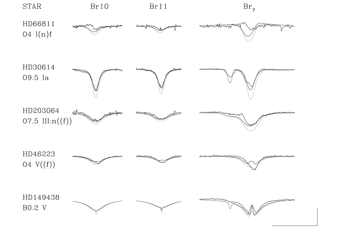
Figure 15: Influence of different collisional cross sections for hydrogen: some prototypical examples. Solid: Best fit with cross sections from Giovanardi et al. (1987), as in Figs. 9 to 11. Grey: Models with identical parameters, but cross sections calculated according to Przybilla & Butler (2004). See text.

8.1 Comments on hydrogen collisional cross sections

In Sect. 3.1 we briefly discussed the importance of consistent collisional data for the resulting IR line profiles. We outlined recent calculations performed by Przybilla & Butler (2004) and references therein. These authors provide a recipe for an “optimum” choice of collisional data, based on a number of comparisons with observations, comprising mostly BA-type dwarfs (including $\tau$ Sco) and supergiants, whereas only one test has been presented for an O-star, the O3.5 dwarf HD 93250.

After incorporating their data into our version of fastwind, we have subsequently tried to analyze our observed dataset. First let us mention that this modification gave rise to changes in the hydrogen lines alone, since in all cases the temperature structure (being dependent on the collisional bound-bound rates) remained almost unaffected, with maximum changes on the order of 100 Kelvin.

Unfortunately, however, it turned also out that, again in all cases, the hydrogen line cores became stronger (in agreement with the findings by Przybilla & Butler), whereas the line wings are barely affected, as shown in Fig. 15 for some prototypical examples taken from the fits in Figs. 9 to 11. In a few cases this might actually lead to an improvement of the situation, e.g., for HD 46223 or Cyg OB2 #8C, which actually need gravities higher than those derived above. (Remember that increasing the gravity results in shallower line cores, cf. Sect. 4.1). Since, however, the IR-gravities based on our standard collisional data from Giovanardi et al. (1987) were found to be consistent with the optical ones in the majority of cases, models based on the alternative data by Przybilla & Butler would consequently lead to an overestimate of gravities.

The same would be true for the mass-loss rates. Using the new data would sometimes improve the situation, e.g., any central emission inside Br_γ (if present) becomes reduced, cf. HD 46233 and $\tau$ Sco in Fig. 15. Actually, this reduction is the origin of the lower mass-loss rate of $\tau$  Sco as derived by Przybilla & Butler (2004): If ${\dot{M}}$ is decreased, the strength of this feature increases again, at least if the winds are very weak, due to subtle NLTE effects and unrelated to any direct wind emission.

For “normal” winds, on the other hand, where wind emission plays the primary role, the deeper cores predicted by the “new” models would necessitate higher mass-loss rates. Thus, the present situation would get worse, at least in those cases where ${\dot{M}}$ is no longer derived exclusively from the wings. As an example, consider HD 203064 in Fig. 15, which presently has an IR mass-loss rate which is a factor of two larger already. Using the new dataset would further deteriorate this discrepancy.

Insofar, the preference for our standard set of collisional data is triggered solely from the results described above, namely from the generally satisfactory agreement between the IR and optical analyses for those objects analyzed in the present investigation. We do not argue that one set or the other is better, but point out that in these cases our standard dataset gives results which are more consistent with the optical.

Of course, we have also looked into some of the details responsible for the differences obtained. It turned out that the NLTE departure coefficients are astonishingly similar, when comparing the results from both collisional datasets. There are only (very) subtle differences in those regions where the line cores are formed giving rise to the deeper profiles if the dataset by Przybilla & Butler is used. Either the lower level of the transition is slightly more populated, or the upper one is slightly less populated. The obvious discrepancies are then induced by the extreme sensitivity of the IR line formation on such subtle differences. As has already been argued about the formation of Hei lines (Sect. 4.2), this discrepancy would barely be visible if the lines were situated in the optical. Insofar, not only the data but also the numerical treatment plays a crucial role. In any case it is quite astonishing how well the observed profiles can be simulated.

9 Summary and conclusions

In this paper, we have analyzed 25 Galactic O and early B-stars by means of H and K band spectroscopy. The primary goal of this investigation was to check to what extent a lone near-IR spectroscopy is able to recover stellar and wind parameters derived in the optical. This is critical to our desire to precisely analyze the hot, massive stars, deep within the disk of our Galaxy, and in particular the very young, massive stars just emanating from their birth places.

Most of the spectra have been taken with subaru-ircs, at an intermediate resolution of 12,000. In order to synthesize the strategic H/He lines present in the H/K band, we have used our recent, line-blanketed version of fastwind. In total, seven lines have been investigated, three from hydrogen, including Br_γ serving as a diagnostic tool to derive wind-densities, two Hei and two Heii lines. For two stars, we could make additional use of Hei2.05 (singlet) which has been observed with irtf-cshell. Apart from Br_γ and Heii2.18, the other lines are predominately formed in the stellar photosphere, and thus remain fairly uncontaminated from more complex physical processes, particularly clumping.

In our attempt to prepare all required broadening functions, it turned out that at present we have to rely on the Griem approximation for Stark broadening (important for hydrogen and Heii), since the corresponding published data (based on the more exact VCS approach) suffer from numerical problems, particularly for the members of higher series.

First we investigated the predicted behaviour of the strategic lines, by means of a large model grid described in Puls et al. (2005). Interestingly and in contradiction to what one expects from the optical, almost all photospheric lines in the H and K band (from H, Hei and Heii ) become stronger if the gravity decreases. In Sect. 4, we have carefully investigated the origin of this rather unexpected behaviour.

Concerning H and Heii, it is related to the particular behaviour of Stark broadening as a function of electron density, which in the line cores is somewhat different for members of lower and higher series. For the latter, the cores become deeper when the density decreases, and contribute more to the total line strength than in the optical.

Regarding Hei, on the other hand, the predicted behaviour is due to some subtle NLTE effects resulting in a stronger overpopulation of the lower level when the gravity decreases, so that the source function becomes weaker and the profile deeper, i.e., stronger. This strong dependence of the profile on the source function is a direct consequence of the IR line formation with $h\nu/kT<<1$. If those lines were situated in the optical, on the other hand, optical depth effects would dominate, leading to a decrease of line strength due to a lower number of Hei absorbers. This explains the different (and “normal”) behaviour of, e.g., Hei4471.

In Sect. 5, we have compared our calculations with results presented recently by Lenorzer et al. (2004), utilizing the alternative NLTE model atmosphere code cmfgen. In most cases, we found reasonable and partly perfect agreement. Only the Hei2.05 singlet for mid O-types suffers from some discrepancy, in agreement with our analogous findings for optical Hei singlets (Puls et al. 2005).

After carrying out the analysis for our sample described above (and in agreement with the predictions from our model grid), we find that an H/K band analysis is able to derive constraints on the same set of stellar and wind parameters as it is known from the optical, e.g., $T_{\rm eff}$, $\log g$, $Y_{\rm He}$ and optical depth invariant $Q$, where the latter yields the mass-loss rate ${\dot{M}}$ if stellar radius and terminal velocity are known. For cooler objects, when Heii is missing, a similar analysis might be possible if Hei2.05 (provided to be described correctly) is available and the helium content can be adopted (due to the almost orthogonal reaction of Hei2.05 and Hei2.11 on $T_{\rm eff}$ and $\log g$). This should be possible for very young objects containing unprocessed material.

For future purposes, when no UV observations will be available, the terminal velocity $v_{\rm\infty}$ has to be taken from calibrations, as it is true for the velocity field exponent $\beta$, at least in those cases when no emission wings in Br_γ are visible. Concerning the determination of $R_{\ast}$, a similar strategy as in the optical might be developed, utilizing infrared colors and distances.

For most of our objects, we obtained good fits, except for the line cores of Br_γ in early O-stars with significant mass-loss (see below), and except for the fact that particularly at mid O-types Br10/11 could not be fitted in parallel. We have argued that this discrepancy is similar to the problem in the optical, concerning Heii4200/4541 (e.g., Herrero et al. 2002). Due to the similarity in the involved levels and broadening functions, we have speculated about a possible defect of these broadening functions for transitions between members of higher series. The largest discrepancy, however, was found for the line cores of Br_γ. First note that this problem is not particularly related to our code, since also cmfgen exhibits the same shortcoming. Whereas the observations show Br_γ mostly as rather symmetric emission lines, the models predict a P Cygni type line, with a comparably deep core which is never observed. Note that this type of profile can only be created if the ratio of departure coefficients for the involved levels (n = 4 $\rightarrow$7) deviates strongly from unity (cf. Puls et al. 1996), whereas a ratio close to unity would just give the observed symmetric emission profile. One might speculate that this can be achieved due to a stronger influence of collisional bound-bound processes, which, e.g., might be possible in a strongly clumped medium. Remember, however, that Br_γ typically forms inside the H_α-”sphere” (Lenorzer et al. 2004), where the degree of clumping is usually thought to be moderate (e.g., Markova et al. 2004; Repolust et al. 2004), though a recent investigation by Bouret et al. (2005) strongly indicates the opposite.

After having derived the stellar and wind parameters from the IR, we have compared them to results from previous optical analyses, in an almost strictly differential way, since most of these results have been obtained also on the basis of fastwind. Overall, the IR results coincide in most cases with the optical ones within the typical errors usually quoted for the corresponding parameters, i.e, an uncertainty in $T_{\rm eff}$ of 5%, in $\log g$ of 0.1 dex and in ${\dot{M}}$ of 0.2 dex, with lower errors at higher wind densities. In most of the cases where we have found discrepancies beyond these errors, their origin could be easily identified. Definite outliers above the 1-$\sigma$ level where found in four cases with respect to $\log g$ and in two cases for ${\dot{M}}$, at intermediate wind-strengths. Given the 1-$\sigma$ character of the discussed errors, these mismatches are still not too worrisome, since all identified discrepancies lie well below 2-$\sigma$, and no trends are visible. Particularly with respect to $\log g$  it is quite possible that errors exceeding the nominal error of 0.1 dex do exist in certain cases, both in the optical and the IR, related to fits which are not at their (global) optimum (e.g., Mokiem et al. 2005). Re-assuring is the fact that the mean difference between NIR and optical gravities is very close to zero, $\Delta\log g=-0.025\pm 0.1$.

As a by-product of our investigation, we could determine the (IR-) stellar parameters and the $\log Q$ value for three dwarfs, which have not been analyzed in the optical so far. Though we have shown that the derived quantities are rather insensitive to uncertainties in $R_{\ast}$ and $v_{\rm\infty}$, these objects need to be checked in the optical.

Let us highlight one additional “bonus” obtained from the infrared. In those cases when a star has an extremely weak wind and the core of Br_γ can be resolved (requiring a very low rotational speed), the central emission will give us a clue about the actual mass-loss rate and not only an upper limit, as is true for the optical. An example of this kind of diagnostics is $\tau$ Sco. Particularly with respect to recent investigations of young dwarfs with surprisingly weak winds (Martins et al. 2004), this will turn out as an invaluable source of information (even more, if coupled with observations of Br_α, e.g. Najarro et al. 1998; Przybilla & Butler 2004).

After finishing this investigation, we are now able to constrain the observational requirements to perform such a detailed IR-analysis (but see below). Most important is a high S/N, because most of the lines to be investigated are extremely shallow, at least for the hotter objects. The resolution must be sufficient to disentangle the line cores from the wings (particularly important for Br_γ) and to obtain reasonable clues about any contamination due to reduction problems. As for the required set of lines, almost all lines analyzed in the present paper are necessary to obtain useful constraints, maybe except for Br10, since Br11 seems to be less contaminated. Since both Heii lines behave very similarly and show the same degree of consistency or disagreement (if present), one of those two lines might be discarded as well.

In the last section of this paper, we have argued that our standard implementation of hydrogen collisional cross sections seems to give results which are in better agreement with the optical results for our sample of hot objects, compared to the data suggested recently by Przybilla & Butler (2004). In view of their findings, namely that for cooler stars their prescription gives more consistent results, this discrepancy has to be clarified in future work. The same of course is true regarding the severe mismatch of the Br_γ cores. A first step will require to include clumping and to investigate to what extent this process might improve the situation.

The value of a reliable quantitative analysis for hot, massive stars based entirely in the infrared cannot be overstated. Most obvious, it will allow the evaluation of massive star characteristics at an evolutionary stage significantly earlier than has ever been possible before. The influence of disk emission may render the photosphere of some very young massive stars inaccessible. We suspect, however, that among the most massive stars, around mid-O or hotter, the disk will be destroyed well before even near-infrared studies would be feasible due to the very short disk lifetime (Watson & Hanson 1997).

A combined H and K band analysis with the S/N we present here won’t always be possible, nor is it required. A S/N of just 150 and resolution of order $R\sim 5000$ will typically be sufficient for a reasonable analysis, provided the star is not a slow rotator (see discussion in Hanson et al. 2005). How deep into the Galaxy one can probe is a strong function of the line of sight extinction and the intrinsic stellar brightness. For late-O dwarfs with $A_{\rm V}\sim 20$, one can only probe a few kiloparsecs. However, for early-O dwarfs or most O and early-B supergiants, even with $A_{V}\sim 20$, one should be able to probe the entire solar circle. For this level of extinction, it is the H band measurements which pose the greatest challenge, though $S/N\sim 120-150$ should still be attainable with an 8-m class telescope. For still redder stars, the H band would be too dim for useful spectra. Once $m_{K}>14-15$ (OB supergiants at the far side of the Galaxy with $A_{\rm V}\sim 30$), the corresponding low S/N for such a dim star wouldn’t allow a robust quantitative analysis, though spectral classification is still possible. Thus, excluding sight-lines where the extinction has become extreme (A_V $>$ 30), nearly every luminous OB star within our Galaxy becomes accessible through near-infrared spectroscopic studies.

One of the powers of quantitative analysis is its ability to determine absolute magnitudes. When OB stars are in clusters, those cluster distances will be robust, giving us clues to the structure and nature of the presently, poorly understood, inner Milky Way. OB stars serve as secondaries to massive compact objects. Because the extinction is typically high for such systems found in the inner Galaxy, a NIR analysis of the OB companion provides the only means for making critical measurements to constrain these fascinating systems. In truth, because many more O stars within our Galaxy are visible in the NIR than the optical by almost two orders of magnitude, the development of a robust quantitative analysis in the infrared will stimulate entirely new, important results on massive stars, their formation and evolution and numerous valuable insights into the inner workings of our Milky Way Galaxy.