Measuring Extinction Curves of Lensing Galaxies

Abstract

We critique the method of constructing extinction curves of lensing galaxies using multiply imaged QSOs. If one of the two QSO images is lightly reddened or if the dust along both sightlines has the same properties then the method works well and produces an extinction curve for the lensing galaxy. These cases are likely rare and hard to confirm. However, if the dust along each sightline has different properties then the resulting curve is no longer a measurement of extinction. Instead, it is a measurement of the difference between two extinction curves. This “lens difference curve” does contain information about the dust properties, but extracting a meaningful extinction curve is not possible without additional, currently unknown information. As a quantitative example, we show that the combination of two Cardelli, Clayton, & Mathis (CCM) type extinction curves having different values of $R_{V}$ will produce a CCM extinction curve with a value of $R_{V}$ which is dependent on the individual $R_{V}$ values and the ratio of V band extinctions. The resulting lens difference curve is not an average of the dust along the two sightlines. We find that lens difference curves with any value of $R_{V}$, even negative values, can be produced by a combination of two reddened sightlines with different CCM extinction curves with $R_{V}$ values consistent with Milky Way dust ($2.1\leq R_{V}\leq 5.6$). This may explain extreme values of $R_{V}$ inferred by this method in previous studies. But lens difference curves with more normal values of $R_{V}$ are just as likely to be composed of two dust extinction curves with $R_{V}$ values different than that of the lens difference curve. While it is not possible to determine the individual extinction curves making up a lens difference curve, there is information about a galaxy’s dust contained in the lens difference curves. If the lens difference curve can be fit with the CCM relationship (regardless of the fitted $R_{V}$ value), this implies that the dust along the two slightlines can be described by CCM. In addition, the presence of the 2175 Å feature in the lens difference curve means that this feature is present along at least one of the two lensed sightlines.

1 Introduction

The well-known Milky Way extinction relation of Cardelli, Clayton, & Mathis (1989, CCM) applies to a wide variety of Galactic interstellar environments. CCM extinction curves are described by one parameter, $R_{V}$, the ratio of total-to-selective extinction in the V band. The $R_{V}$ value is a rough measure of average dust grain size, and therefore provides a physical basis for the variations in extinction curves. For the Galaxy, the often-quoted average $R_{V}\simeq 3.1$, merely reflects the typical value for dust along diffuse sightlines. But the diverse environments within the Milky Way show a range of values, $2.1\leq R_{V}\leq 5.6$ (Valencic, Clayton, & Gordon 2004). A Milky Way UV extinction curve is characterized by a “bump” at 2175 Å and a rise in the far-UV. While CCM applies to most sightlines in the Milky Way and a few in the Magellanic Clouds, it does not typically apply in other extragalactic environments where extinction curves have been measured (Gordon et al. 2003; Gordon, Calzetti, & Witt 1997; Pitman, Clayton, & Gordon 2000).

Traditionally, the pair method is used to determine extinction by comparing the spectral energy distributions (SEDs) from reddened and unreddened stars of the same spectral type (Massa, Savage, & Fitzpatrick 1983). The pair method has only been applied within Local Group galaxies such as the Milky Way, SMC, LMC, and M31 because it is necessary to use individual stars as point sources. Determining extinction in galaxies beyond the Local Group is generally a more complex problem. Any surface photometry of a galaxy contains light from a mixture of gas, dust, and stars, making it difficult to analyze the spectral energy distributions from these complex systems directly. To derive the SED of a galaxy requires a radiative transfer model which accounts for the physical properties of the dust, the stellar population, and the geometrical distribution of the dust within the galaxy (e.g., Gordon et al. 2001; Misselt et al. 2001). Applied to starburst galaxies, these models imply that these galaxies have dust with properties more similar to that in the SMC than to the Galaxy, having no measurable 2175 Å bump (Calzetti, Kinney, & Storchi-Bergmann 1994; Gordon et al. 1997). The existence of the CCM relation in the Galaxy, valid over a large wavelength interval, suggests that the environmental processes that modify the grains are efficient and affect all grains. In other galaxies, environmental processing by radiation and shocks near regions of star formation or variations in galactic metallicity may be responsible for the large observed variations in extinction curve properties from CCM (e.g., O’Donnell & Mathis 1997; Gordon & Clayton 1998). Certainly, the application of the CCM extinction law for Galactic dust is not appropriate for dust in starburst galaxies and it is unkown if it is appropriate for dust in more quiescent galaxies.

In order to study extinction in galaxies beyond the Local Group, a new method has been developed. It uses multiply imaged QSOs produced by gravitational lensing to study the extinction properties of the lensing galaxy (Nadeau et al. 1991). The multiple images originate from the same QSO and thus have the same intrinsic SED. Therefore, this seems ideal for constructing extinction curves by the pair method. The different images are produced by light traveling along different sightlines through the lensing galaxy, so the amount of reddening varies from image to image. The SEDs of the two images are then compared using the pair method to determine an extinction curve for the lensing galaxy. In this paper, we investigate the usefulness of this method in producing extinction curves of lensing galaxies.

2 Background

The literature currently contains $\sim$25 multiply imaged QSOs, listed in Table 1, for which extinction curves have been calculated, using either spectroscopic or photometric data. Typically, a CCM relation was fit to these curves and a value of $R_{V}$ found. Gravitational lensing is an achromatic process, but often the various images of a QSO are found to have different colors. The color differences are likely due to reddening by dust in the lensing galaxy (Yee 1988). Each image produced by a gravitational lens is also magnified by a different amount depending on the geometry of the source, and the lens, and possibly amplified due to microlensing effects. Early work by Nadeau et al. (1991) on the lens system Q2237+0305 showed that each of four images from a single QSO source had different colors, and a method for determining the extinction was suggested. In order to find $A(\lambda)/A(V)$, the ratio of total extinction at a given wavelength, $\lambda$, to the total extinction in the V-band, directly from the ratio of fluxes from two images, it is necessary to know the amplification ratio. Since the amplification ratios are uncertain, they assumed a value of $A(\lambda)/A(V)$ at the central wavelength of the K-band. Because the images only differed in magnitude by a small amount, Nadeau et al. assumed that the extinction at any given wavelength differs only slightly from the average Galactic extinction law. Nadeau et al. (1991) determined an extinction law for the lensing galaxy using the assumption that $A(K)/A(V)=0.11$, the Galactic value (Clayton & Mathis 1988). The resulting extinction curve is remarkably similar to the $R_{V}=3.1$ Galactic extinction curve, for $0.5\lesssim\lambda^{-1}\lesssim 2\,\micron^{-1}$.

Falco et al. (1999) built upon the work by Nadeau et al. (1991) and completed the first survey of extinction properties of 23 lensing galaxies. Using photometric data for multiply imaged QSOs, Falco et al. determined the differential extinction, $\Delta E(B-V)$, for each set of images. The process of determining differential extinction depends on several assumptions. First, they assumed that the source spectrum (from the QSO) is identical for each image. Second, they assumed that the spectrum does not show significant time variability over a span equal to the time delay for the images. Finally, they assumed that the magnification, $\Delta M$, by the lens does not depend on wavelength or time. In order to compare the images, the magnification of one image was set to one, and the extinction of the bluest image set to zero. In several cases, Falco et al. use radio data to determine $\Delta M$. They use some spectroscopic redshifts, but also use a technique suggested by Jean & Surdej (1998) to determine photometric redshifts for several lenses. It should be noted that microlensing effects are not considered here, but Falco et al. suggested that these effects are small compared to the mean magnification, which is constant and achromatic. In many cases for which radio data were unavailable, the differential magnification, $\Delta M$, was treated as a free parameter when determining the best fit extinction curve. Extinction curves have also been calculated from multiply imaged QSOs by Toft, Hjorth, & Burud (2000), Motta et al. (2002), and Munoz et al. (2004).

Motta et al. (2002) use spectroscopic data to determine differential extinction in the lens galaxy SBS 0909+532. They suggested that spectroscopy is more suitable for the study of extinction in lenses because broadband photometry sometimes makes extinction and gravitational microlensing indistinguishable. Microlensing causes the flux for a single image to increase inhomogeneously across the wavelength range of an individual filter, affecting the color of the individual image. Using spectroscopy allowed them to overcome many of the challenges presented by photometric methods. Wucknitz et al. (2003) used spectra of the doubly imaged QSO HE 0512-3329 to distinguish between the effects of extinction and microlensing. Because extinction affects the emission lines, but microlensing does not, the emission lines can be used to separate these effects. Then, the continuum, which is affected by both microlensing and extinction, can be corrected for extinction and the microlensing effects may be studied directly. While extinction curves were not the focus of this paper, they fit the CCM relation to their data. They treated $R_{V}$ as a free parameter, and fit their data using several values of $\Delta E(B-V)$ and $\Delta A(V)$. They suggested that the measured extinction curve could be the result of dust with two different values of $R_{V}$ along the two sightlines.

Each of the papers cited above uses roughly the same method for obtaining an extinction curve by the pair method. When calculating the extinction curve, they consider $R_{V}$ to be a free parameter as well as the magnification, if it is not known. For several of the lensing systems, observations in the radio, where extinction is negligible, allow for a direct measurement of the differential magnification ($\Delta M$). The magnitudes of two images, labeled A and B, at wavelength $\lambda$, are compared using the equation

$$m_{B}(\lambda)-m_{A}(\lambda)=\Delta M+\Delta E(\lambda)R(\frac{\lambda}{1+z_{l}})$$ (1)

where $\Delta E$ is the differential reddening, and $R$ is the ratio of total-to-selective extinction for the given wavelength and lensing galaxy redshift (Motta et al. 2002). This is similar to the traditional pair method where $m_{B}(\lambda)-m_{A}(\lambda)=\Delta E(\lambda)R(\lambda)=A(\lambda)$. The lensing galaxy extinction curves are typically presented unnormalized making it difficult to compare these results to other extinction studies. Extinction curves should to be normalized to $E(B-V)$ or $A(V)$ so that only the wavelength dependence, not the amount of extinction, is compared. In this paper, all plots are presented in rest wavelength space and with the extinction normalized to $A(V)$. It is straightforward to determine the normalized extinction using the following equation

$$\frac{A(\lambda)}{A(V)}=\frac{m_{B}(\lambda)-m_{A}(\lambda)-\Delta M}{\Delta E(B-V)R_{V}}$$ (2)

3 Discussion

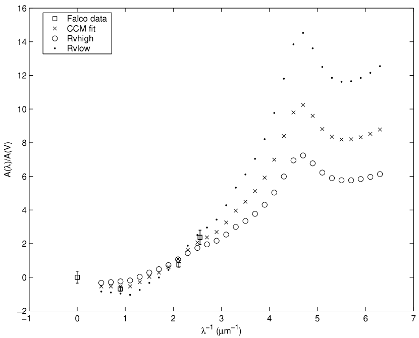
Figure 1: Extinction data for B1600+434 (squares) fitted with a CCM curve with $R_{V}=0.92$ (crosses) from Falco et al. (1999). Additional CCM extinction curves are plotted with Rvlow=0.65 and Rvhigh=1.3. This plot shows how weakly constrained the “fitted” CCM extinction curve is. The data are presented in rest wavelength space.

Figure 1 shows a normalized extinction curve for one of the lenses, B1600+434 (Falco et al. 1999). Using the photometric data in Falco et al., as well as their values for $R_{V}$, $\Delta E(B-V)$, and redshift, we plot the data and the fit which has an extremely low $R_{V}=0.92$. As pointed out by Falco et al. and shown in the figure, the small number of photometric points covering a limited wavelength range can be fit with CCM curves showing a very large range of $R_{V}$ values.

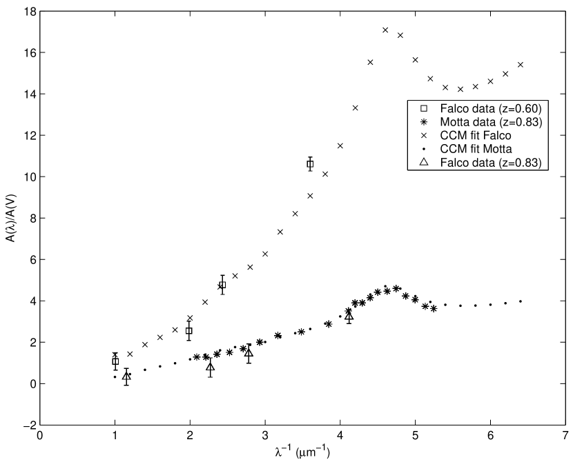
Figure 2: Motta et al.(2002) and Falco et al.(1999) data for SBS 0909+532 shown with CCM fits for $R_{v}=2.1$, the value obtained in the fit by Motta et al., and $R_{V}=0.64$, the value reported by Falco et al. for their best-fit extinction curve. Also plotted are the Falco data using the Motta redshift and normalization, $A(V)$. All data have been transformed into rest wavelength space using the reported redshifts.

The results for the extinction curve given in Motta et al. (2002) for SBS 0909+532 differ greatly from those given by Falco et al. (1999) for the same QSO. In fact, the differential extinction is similar (both reported values around $\Delta E(B-V)=0.2$) but the inferred values for $R_{V}$ are different. Falco et al. (1999) used an estimated redshift of $z=0.60$ for the lensing system and get $R_{V}=0.64\pm 0.15$. Their data and the CCM extinction curve with the reported $R_{V}$ value are shown in Figure 2. Motta et al. (2002) used a lens redshift of $z=0.83$, found spectroscopically by Oscoz et al. (1997) using the Mg II absorption doublet and found $R_{V}=2.1\pm 0.9$. If the extinction curve data given in Falco et al. (1999) are transformed to the same redshift as Motta et al. (2002) and normalized with the proper $A(V)$, the data fall right on the curve suggested by Motta as seen in Figure 2. Falco et al. (1999) point out that using the technique of Jean & Surdej (1998) does not always lead to accurate redshift and that using the wrong redshift will produce an incorrect extinction curve. Therefore, extinction curves produced from data with uncertain redshifts are not necessarily useful.

Two important assumptions, made by all the studies listed in Table 1, are that one sightline is less reddened than the other, and that both sightlines have dust with the same extinction properties, i.e., the same value of $R_{V}$. If both images of the QSO are reddened but with different values of $R_{V}$ then combining them to produce an extinction curve is not so straightforward. The wavelength dependence of dust extinction in any galaxy is unknown a priori, but for simplicity let’s assume it follows the CCM relation.

The CCM relationship at any wavelength, $\lambda$, is:

$$\frac{A(\lambda)}{A(V)}=a(\lambda)+\frac{b(\lambda)}{R_{V}}.$$ (3)

Let’s assume that each QSO image has a dust column with different amounts and $R_{V}$ values. Then, the magnitude difference between two lensed images is:

$$A(\lambda) = \left[\frac{A_{2}(\lambda)}{A_{2}(V)}\right]A_{2}(V)-\left[\frac{A_{1}(\lambda)}{A_{1}(V)}\right]A_{1}(V)$$ (4)

$$= \left[a(\lambda)+\frac{b(\lambda)}{R_{V2}}\right]A_{2}(V)-\left[a(\lambda)+\frac{b(\lambda)}{R_{V1}}\right]A_{1}(V)$$ (5)

$$= \left[A_{2}(V)-A_{1}(V)\right]a(\lambda)+\left[\frac{A_{2}(V)}{R_{V2}}-\frac{A_{1}(V)}{R_{V1}}\right]b(\lambda)$$ (6)

where $R_{V1}$ and $A_{1}(V)$ give the dust properties of the least attenuated, “unreddened”, image and $R_{V2}$ and $A_{2}(V)$ of the most attenuated, “reddened”, image (Wucknitz et al. 2003). Normalizing the extinction at any wavelength by the amount of extinction in the V-band gives:

$$\frac{A(\lambda)}{A_{2}(V)-A_{1}(V)}=a(\lambda)+\left[\frac{A_{2}(V)}{A_{2}(V)-A_{1}(V)}\frac{1}{R_{V2}}-\frac{A_{1}(V)}{A_{2}(V)-A_{1}(V)}\frac{1}{R_{V1}}\right]b(\lambda).\\$$ (7)

Equation 7 gives the extinction curve that is actually measured for our simple example. It is the CCM relationship with an $R_{V}$ value of

$$\frac{1}{R_{V12}} = \frac{A_{2}(V)}{A_{2}(V)-A_{1}(V)}\frac{1}{R_{V2}}-\frac{A_{1}(V)}{A_{2}(V)-A_{1}(V)}\frac{1}{R_{V1}}$$ (8)

$$= \left[\frac{1}{1-\frac{A_{1}(V)}{A_{2}(V)}}\right]\frac{1}{R_{V2}}-\left[\frac{1}{\frac{A_{2}(V)}{A_{1}(V)}-1}\right]\frac{1}{R_{V1}}$$ (9)

Therefore, the combination of two CCM extinction curves is also a CCM extinction curve but the resulting value of $R_{V}$ is not an average of $R_{V1}$ and $R_{V2}$. Thus, the measurement of the difference between two lensed sightlines is actually the difference of two extinction curves, not an extinction curve itself. In order to avoid confusion, we propose the term “lens difference curve” be used for these measurements instead of labeling them extinction curves which can be misleading.

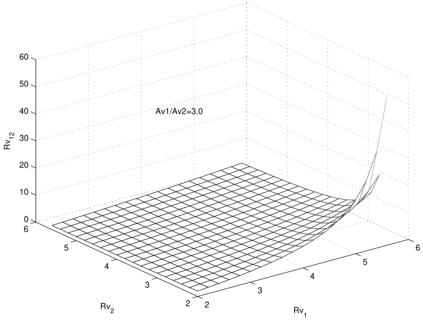
Figure 4: For any fixed ratio, $A_{1}(V)/A_{2}(V)$, it is possible to obtain a wide range of combined $R_{V}$ values, $R_{V12}$. For this fixed value of $A_{1}(V)/A_{2}(V)=3$, we find $1.5\lesssim R_{V12}\lesssim 56$.

As a quantitative example, in Figure 3 we show the lens difference curve for B0218+357, described by Munoz et al. (2004) with $R_{V}=12$, fit to 6 photometric data points. We have reproduced this lens difference curve with a combination of different dust types for each image having $R_{V}=5.5$ and $2.7$. This result is not in any way unique. In fact, a very wide range of values of $R_{V12}$, can be produced by varying the values of $R_{V1}$ and $R_{V2}$. An example is shown in Figure 4, with $A_{1}(V)/A_{2}(V)=3$. For this choice of $A_{1}(V)/A_{2}(V)$, we find $1.5\lesssim R_{V12}\lesssim 56$. Similar results are seen for other values of $A_{1}$(V)/$A_{2}$(V). It is even possible to produce negative values of $R_{V}$ for such lens difference curves (Wucknitz et al. 2003).

In general, for any two QSO images, the value of $A_{1}$(V)/$A_{2}$(V) is unknown. This highlights the main difference between the pair method as applied to lensing galaxies and the pair method as applied to stars in the Galaxy and the Magellanic Clouds (Valencic et al. 2004; Gordon et al. 2003). In the latter case, the reddening, E(B-V), and the ratio of total-to-selective extinction, $R_{V}$, can be independently measured along the sightline to each star so that $A_{1}$(V)/$A_{2}$(V) is a known quantity. Then, a unique extinction curve, within the measurement uncertainties, can be derived. Only in two limiting cases will the pair method produce an actual extinction curve for QSO images. First, if the wavelength dependence of the extinction is the same for dust along both sightlines then the resulting lens difference curve will be an extinction curve. In our simple CCM example, if the value of $R_{V}$ is the same for the dust along both sightlines, then equations 7 and 9 produce a correct extinction curve and $R_{V}$ value. Second, if $A_{2}$(V) $>>$ $A_{1}$(V) then it doesn’t matter if the extinction parameters are different for the dust along the two sightlines. In this case, equations 7 and 9 again produce the correct values when $A_{1}$(V) is set to zero.

So the pair method for lensing galaxies can work but generally it is unknown which individual pairs of QSO images either have the same $R_{V}$, or have one image that is much more reddened than the other. Several hundred sightlines within the Milky Way have measured extinction curves (Valencic et al. 2004). The so-called average Milky Way extinction curve with $R_{V}$=3.1 is, in fact, the typical extinction for diffuse sightlines in the Galaxy. It is not in any way an average curve for the Galaxy. Any two sightlines widely spaced in the Galaxy are likely to have very different values of $R_{V}$. The lensed QSO, B0218+357, where one sightline passes through a molecular cloud, is a case in point (Munoz et al. 2004). If the second sightline is lightly reddened then an accurate extinction curve for the dust in this molecular cloud is being produced. But if the second sightline is also significantly reddened but with dust from the more diffuse interstellar medium in the intervening galaxy, then the resulting measurement is a lens difference curve not an extinction curve. This lens difference curve reflects the difference in the two sightlines’ extinction curves and it is nontrivial to extract the original extinction curves from the lens difference curve. A very wide range of $R_{V}$ values is listed for the lensing galaxies in Table 1. Some fall in the normal range seen for Galactic sightlines, between $2.1$ and $5.6$, while other values are quite extreme. However, as can be seen from Figure 4, the normal Galactic values in Table 1 are no more likely to be correct than the extreme values.

While it is not possible to extract the extinction curves from a lens difference curve, there is information about the dust in the lensing galaxy contained in the lens difference curve. While it may be possible to create a lens difference curve which follows the CCM relationship without the two individual extinction curves also following the CCM relationship, this seems unlikely. Therefore, if the lens difference curve can be fit with the CCM relationship regardless of the $R_{V}$ value, this is evidence that the dust in the lensing galaxy follows the CCM relationship. In addition, if the 2175 Å extinction bump is present in the lens difference curve, then there must be bump dust in the more reddened sightline at least. Munoz et al. (2004) focus on the extinction bump at 2175 $\AA$. Lens difference curves are shown for LBQS 1009-0252 and B0218+357, and the latter shows a bump at 2175 Å which is reproduced here in Figure 3. Motta et al. (2002) also found the bump in their lens difference curve for SBS 0909+532. The presence of the bump in these lens difference curves implies that there is Milky Way-type bump dust, not just SMC-type dust along at least one of the component sightlines.

Just because we do not see very large or very small values of $R_{V}$ in the Local Group galaxies doesn’t mean that exotic dust with very different properties can’t exist in distant galaxies. Very simplistically, a small $R_{V}$ implies that a greater mass fraction is contained in small dust grains and vice versa. However, extinction by large grains is less efficient than extinction by small grains because mass scales as $a^{3}$ while surface area scales as $a^{2}$. Therefore, for any given gas abundance of grain materials and gas-to-dust-ratio, large grains will use a much higher fraction of the available material in order to produce the same amount of extinction. For instance models for dust along Galactic sightlines having high $R_{V}$, such as the Orion sightline HD 37022 ($R_{V}=5.5$), tend to run out of material to build large grains (Clayton et al. 2003). Therefore in general, sightlines with very small values of $R_{V}$ are more likely to be physically possible than very large $R_{V}$ values.

4 Conclusions

• In general, the difference between two lensed sightlines in a galaxy does not produce an extinction curve, but a lens difference curve. It is not easy to decompose this lens difference curve into the two sightline extinction curves.

• We show that the combination of two CCM type extinction curves having different values of $R_{V}$ will produce a lens difference curve which follows the CCM relationship. The $R_{V}$ value of the lens difference curve is a function of the $R_{V}$ values of the individual lensed sightlines and the ratio of their V band attenuations.

• If one of the two QSO images is lightly reddened or if the dust along both sightlines has the same extinction wavelength dependence then the lens difference curve is an accurate extinction curve for the lensing galaxy.

• Lens difference curves can only be accurately constructed for lenses with known redshift and magnification ratio, $\Delta M$. If the redshift is wrong, the lens difference curve is wrong.

• A small wavelength coverage results in lens difference curve CCM fits that are not well constrained.

• The presence of a “bump” at 2175 Å in a lens difference curve implies that there is Milky Way-like dust along at least one of the sightlines.

• An accurate CCM fit to a lens difference curve, regardless of the fitted $R_{V}$ values, implies that the two lensed sightlines have CCM-like dust extinction curves.

Table 1: Summary of Recent Work

object	$R_{V}$	$\Delta E(B-V)$	z	$\Delta M$	Reference
		(mag)
Q0142-100	$3.11\pm 1$	-0.06	0.49	$\cdots$	1
B0218+357	$7.2\pm 0.08$	0.62	0.68	$1.4\pm 0.03$	1
	$12\pm 2$	0.30	0.6847	$1.4\pm 0.3$	2
MG 0414+0534	$1.47\pm 0.15$	1.41	0.96		1
	1.8	$\cdots$	(1.15)	$\cdots$	3
SBS 0909+532	$0.64\pm 0.15$	0.19	(0.60)	$\cdots$	1
	$2.1\pm 0.9$	0.20	0.83	$-0.2\pm 0.2$	4
FBQ 0951+2635	$4.86\pm 0.85$	-0.03	(0.30)	$1.67\pm 0.22$	1
BRI 0952-0115	$3.1\pm 1$	0.12	(0.55)	$\cdots$	1
Q0957+561	$6.63\pm 0.87$	-0.05	0.36	$\cdots$	1
LBQS 1009-0252	$2.72\pm 0.84$	-0.14	(0.60)	$\cdots$	1
	$2.5\pm 0.3$	0.41	(0.88)	$1.3\pm 0.1$	2
Q1017-207=J03	$3.1\pm 1$	-0.03	(0.60)	$\cdots$	1
B1030+074	$3.1\pm 1$	0.38	0.6	$0.32\pm 0.04$	1
HE 1104-1805	$2.87\pm 0.96$	-0.14	(0.80)	$\cdots$	1
PG 1115+080	$2.89\pm 0.99$	-0.02	0.31	$\cdots$	1
Q1208+1011	$3.47\pm 0.97$	0.07	(0.60)	$\cdots$	1
HST 12531-2914	$3.1\pm 1$	$\cdots$	(0.81)	$\cdots$	1
H1413+117	$2.94\pm 0.66$	0.22	(0.70)	$\cdots$	1
	9	$\cdots$	(1.15)	$\cdots$	3
HST14176+5226	$3.1\pm 1$	$\cdots$	0.81	$\cdots$	1
B1422+231	$2.91\pm 0.81$	0.35	0.34	$\cdots$	1
SBS 1520+530	$2.83\pm 0.96$	-0.19	(0.49)	$\cdots$	1
B1600+434	$0.92\pm 0.58$	0.22	0.42	$0.29\pm 0.1$	1
PKS 1830-211	$6.34\pm 0.16$	0.57	0.89	$0.46\pm 0.06$	1
MG 2016+112	$2.8\pm 0.78$	-0.01	1.01	$-0.06\pm 0.06$	1
HE 2149-2745	$3.08\pm 1$	-0.07	(0.49)	$\cdots$	1
Q2237+0305	$5.29\pm 0.82$	0.13	0.04	$\cdots$	1
	2.8	$\cdots$	(0.13)	$\cdots$	3
B1152+199	$1.8\pm 0.4$	1	0.44	1.21	5

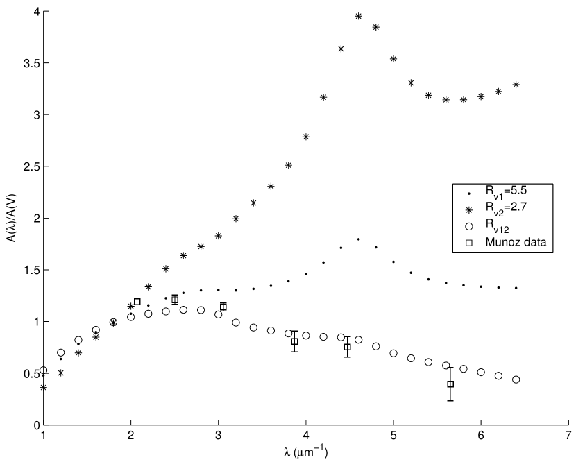
Figure 3: Plot includes data from Munoz et al.(2004) for B0218+357, which fits a CCM ($R_{V}=12$) extinction curve to photometric data in rest wavelength space. This plot shows two extinction curves with the following parameters: $R_{V1}=5.5$, $R_{V2}=2.7$, $E(B-V)_{1}=0.7$, $E(B-V)_{2}=0.4$ as well as the combined curve that would result which has $R_{V12}\approx 12$. Note that the choice of $R_{V1}$ and $R_{V2}$ are not unique. See text.

References

- (1)
- (2) Calzetti, D., Kinney, A. L., & Storchi-Bergmann, T. 1994, ApJ, 429, 582
- (3) Cardelli, J. A., Clayton, G. C., & Mathis, J. S. 1989, ApJ, 345, 245
- (4) Clayton, G. C. & Mathis, J. S. 1988, ApJ, 327, 911
- (5) Clayton, G. C., Wolff, M. J., Sofia, U. J., Gordon, K. D., & Misselt, K. A. 2003, ApJ, 588, 871
- (6) Falco, E. E et al. 1999, ApJ, 523, 617
- (7) Fitzpatrick, E. L. & Massa, D. 1990, ApJS, 72, 163
- (8) Gordon, K. D., Calzetti, D., & Witt, A. N. 1997, ApJ, 487, 625
- (9) Gordon, K. D. & Clayton, G.C. 1998, ApJ, 500, 816
- (10) Gordon, K. D., Clayton, G. C., Misselt, K. A., Landolt, A. U., & Wolff, M. J. 2003, ApJ, 594, 279
- (11) Gordon, K. D., Clayton, G. C., Witt, A. N., & Misselt, K. A. 2000, ApJ, 533, 236
- (12) Gordon, K. D., Misselt, K. A., Witt, A. N., & Clayton, G. C. 2001, ApJ, 551, 269
- (13) Jean, C., & Surdej, J. 1998, A&A, 339, 729
- (14) Massa, D., Savage, B.D., & Fitzpatrick, E. L. 1983, ApJ, 266, 662
- (15) Misselt, K. A., Gordon, K.D., Clayton, G.C., & Wolff, M.J. 2001, ApJ, 551, 277
- (16) Motta, V. et al. 2002, ApJ, 574, 719
- (17) Munoz, J. A., Falco, E. E., Kochanek, C. S., McLeod, B. A., & Mediavilla, E. 2004, ApJ, 605, 614
- (18) Nadeau, D., Yee, H. K. C., Forrest, W. J., Garnett, J. D., Ninkov, Z., & Pipher, J. L. 1991, ApJ, 376, 430
- (19) O’Donnell, J.E., & Mathis, J.S 1997, ApJ, 479, 806
- (20) Oscoz, A., Serra-Ricart, M., Mediavilla, E., & Buitrago, J. 1997, ApJ, 491, L7
- (21) Pitman, K. M., Clayton, G.C., & Gordon, K. D. 2000, PASP, 112, 537
- (22) Toft, S., Hjorth, J., & Burud, I. 2000, A&A, 357, 115
- (23) Valencic, L., Clayton, G. C., & Gordon, K. D. 2004, ApJ, 616, 912
- (24) Wucknitz, O., Wisotzki, L., Lopez, S., & Gregg, M. D. 2003, A&A, 405, 445
- (25) Yee, H. K. C. 1988, AJ, 95, 1331
- (26)