*

Abstract

All fundamental physical principles are confirmed by numerous experiments and practical certainty and have unambiguous interpretation. But physics of stars is based on few measured effects only. It gives some freedom for figments of the imagination. The goal of this paper is to compare two alternative astrophysical models with measurement data.

PACS: 64.30.+i; 95.30.-k

1 Introduction

All basic problems of physics are thoroughly examined. The total accuracy of their solutions is confirmed by numerous direct experiments and their practical using. Any alterative approach to these basic problems seems not to be reasonable. At the first sight it must be applicable to astrophysics too, because it is a part of physics. But the situation here ia quite different. It is accepted in astrophysical community to consider the basis of modern astrophysics as absolutely reliable and steady. But this basis was developed in the past, when there were no possibilities to check them by measuring stellar parameters and many branches of physics, like plasma physics, did not exist. It forces to revisit the basis of stellar physics intently. Nowadays there is possibility to check basic astrophysical problems by means of comparison of theoretical models with measurement data. The astronomers are able to observe and to measure a few parameters of stellar radiation and stellar moving, which obviously depend on the state of stellar interior. In the first place there are parameters of following phenomena:

(1) the apsidal rotation in binary stars

(2) the spectral dependence of solar seismical oscillations.

From this point of view one can consider also the measurement of solar neutrino flux as one of similar phenomenon. But its result can be interpreted ambiguously because there are a bad studied mechanism of their mutual conversation and it seems prematurely to use this measurement for a stellar models checking.

2 Two models of stellar interior

It is generally accepted to think that the equilibrium of substance inside a star can be described by the Euler equation:

$${\mathbf{\nabla}}P+\gamma{\mathbf{g}}=0,$$ (1)

where ${\mathbf{g}}$ is the gravity acceleration, $P$ is the pressure and $\gamma$ is the substance density. Here the density satisfies

$$-4\pi G\gamma=div~{}\mathbf{g},$$ (2)

where $G$ is the gravity constant. Based on this equation astrophysicists supposed that the pressure and the temperature inside a star are growing monotonic with the increase of the depth. As plasma inside a star can be considered as an ideal gas at the pressure $P=n~{}kT$ (n and T are its density and temperature), it is supposed by all astrophysical models that the temperature and the plasma density grow in direction to the star center. Here the temperature reaches tens millions Kelvin and the density is approximately hundred times greater than its averaged value. It is a fundamental statement of modern astrophysics. It is important to underline that although the matter inside a star can be described as an ideal gas, it is not a gas. It is electron-nuclear plasma. Historically the Euler equation (Eq.(1)) was formulate and applied to the astrophysical objects at the time when the term ”plasma” did not exist and basic concepts of plasma physics were not developed. The features of electron-nuclear plasma can not be described by this equation. The equilibrium state in general case must take into account the balance of all forces applied to the system. As particles of plasma have masses and electric charges, the gravity action on plasma can induce its electric polarization $\mathcal{P}$. Taking into account the gravity induced electric polarization (GIEP), the equilibrium equation obtains the form:

$${\mathbf{\nabla}}P+\gamma{\mathbf{g}}+4\pi{\mathcal{P}}~{}div{\mathcal{P}}=0$$ (3)

Analyzing this equation, it is easy to see that there are at last two possibilities. At first, the plasma body can exist in self gravitating field in a state (which can be called Eulerian), when ${\mathcal{P}}=0$ and an equilibrium is determined by Eq.(1). But another equilibrium state is possible when the gravity force is balanced by the electric force:

$$\gamma{\mathbf{g}}+4\pi{\mathcal{P}}~{}div{\mathcal{P}}=0$$ (4)

and the pressure inside the plasma body is constant:

$${\mathbf{\nabla}}P=0.$$ (5)

(The density of plasma under this condition must be constant too $\gamma=const$). Since the polarisation which is non-uniformly distributed in space, can be considered as a distribution of ”bond”charges

$$div\mathcal{P}=\rho_{bond},$$ (6)

we can rewrite the equilibrium condition in the following way:

$$\gamma{\mathbf{g}}+\rho_{bond}~{}E=0$$ (7)

where the intensity of the electric field can be expressed through the density of ”bond”charge:

$$4\pi\rho_{bond}=div~{}\mathbf{E}.$$ (8)

and we can describe further the equilibrium state by Eq.(7) which looks as more convenient at consideration.

The theoretical consideration based on the Thomas-Fermi approximation [2] states that the hot dense plasma in a gravity field must have the equilibrium at the following value of the bond charge electric density:

$$\rho_{bond}=G^{1/2}\gamma$$ (9)

and at the electric field intensity

$${\mathbf{E}}=\frac{\mathbf{g}}{G^{1/2}}$$ (10)

3 The equilibrium of plasma at GIEP effect

3.1 The equilibrium density of hot electron-nuclear plasma

The self-gravity of a celestial body tends to compress the plasma in its central region. In this compressing a plasma density reaches up to $10^{26}$ $particles/cm^{3}$. Such a density corresponds to a minimum of the plasma energy [2]. At temperatures about tens million Kelvin, plasma can be considered as an ideal gas. In accordance with the ideal gas definition, plasma particles interactions are neglected in this approximation. To take into account these interactions in next step of approximation, one can see that two mechanisms of interaction play the most important role.

1) Electrons are Fermi-particles, and they obey the Fermi-statistics. They can not occupy levels in the energetic distribution which another electrons have taken. The value of correction for this interaction is known, it is given in Landau-Lifshitz course [1]. This correction is proportional to the density of particles in the first power and it is positive, therefore when one takes it into account, the plasma energy in this approximation is greater than the ideal gas energy at the same density and temperature.

2)Electrons and nuclei have uniform space distribution at very high temperatures (when interactions can be neglected completely). The same correlation in the space distribution between plasma particles appears at finite temperatures. It can be described by introducing a correlation correction which takes into account electrostatic interaction between nuclei and electrons. This correction is considered in Landau-Lifshitz course [1]. This correction is proportional to particle density in 1/2 and it is negative, therefore taking it into account leads to the decreasing of the plasma energy in comparison with the ideal gas energy at the same density and temperature. If both these corrections are taken into account, we can see that there is a minimum of plasma energy at its density [2]:

$$\eta=\frac{16}{9\pi}\frac{(Z+1)^{3}}{r_{B}^{3}}$$ (11)

Where $Z$ is the averaged charge number of nuclei from which plasma consists, $r_{B}=\frac{\hbar^{2}}{m_{e}e^{2}}$ is Bohr radius. The existing of equilibrium plasma density $\eta$ is not caused by GIEP effect directly. The conclusion about equilibrium density of hot plasma can be deduced from the standard statistical theory and has general meaning. Taking into account GIEP effect one concludes that the plasma density is constant. For equilibrium state this density is obviously equal to $\eta$ because it corresponds to the energy minimum.

The equilibrium state with the density $\eta$ is inherent to the dense plasma at high temperature (about $10^{7}$ K). This temperature is characteristic for central region of a star only. It leads to the conclusion that the core with density $\eta$ is placed in central region of a star and outside of the core there is a region where $\nabla P\neq 0$ and the density and the temperature are change to values which are characteristic for the star surface.

3.2 Another equilibrium parameters of star cores

The constancy of the pressure ($\nabla P=0$), which is characteristic for star cores, needs the constancy of the temperature ($\nabla T=0$). The value of the equilibrium temperature can be extracted from the temperature dependence of the energy. The temperature dependence of the star has two branches with different slopes. At high temperature, when the energy of radiation has a important role, a star as a whole has a positive heat capacity: its energy increases with increasing of its temperature. At a relatively low temperature the heat capacity of a star is negative. Here the star energy decreases while its temperature increases. This behavior of stellar heat capacity is a well known fact, it is discussed in Landau-Lifshitz course [1]. Of course, the own heat capacity of the star substance in each small volume is positive. One obtains the negative heat capacity of a star as a whole at taking into account the gravitational interaction. There is a minimum of the energy placed between these two branches of the temperature dependence of the energy with positive and negative slopes. It determines the equilibrium temperature of the star core [2]:

$${\mathbb{T}}\approx 2\cdot 10^{7}(Z+1)~{}K.$$ (12)

A similar argumentation gives a possibility to determine the equilibrium mass and the equilibrium radius of star core [2].

4 The apsidal rotation in binary stars

4.1 The rotation of close double stars at Eulerian distribution of substance

The apsidal rotation (or periastron rotation) of close binary stars is a result of their non-Keplerian moving which originates from the non-spherical form of stars. This non-sphericity has been produced by a rotation of stars about their axes or by their mutual tidal effect. The second effect is usually smaller and can be neglected. The first and basic theory of this effect was developed by A.Cleirault in the beginning of XVIII century. Now this effect was measured for approximately 50 double stars. According to Clairault’s theory the velocity of periastron rotation must be approximately in 100 times faster if a matter is uniformly distributed inside a star. Reversely, it would be absent if all star mass is concentrated in a star centrum. To reach an agreement between the measurement data and calculations, it is necessary to assume that the density of the substance grows in direction to the centrum of a star and here it runs up a value which is a hundred times greater than a mean density of the star. Just the same mass concentration of the stellar substance is supposed by all standard theories of a star interior. It has been usually considered as a proof of astrophysical models. But it can be considered as a qualitative argument. To obtain a qualitative agreement between theory and measurements, it is necessary to fit parameters of the stellar substance distribution in each case separately.

4.2 The apsidal motion of close binary stars at taking into account the GIEP effect

In the absence of rotation a star would have a spherical core. The rotation transforms it in a oblate ellipsoid. Its oblateness can be calculated [3] and the velocity of periastron rotation can be obtain according to Clairault formulas:

$$\frac{\mathcal{P}}{\mathcal{U}}\biggl{(}\frac{\mathcal{P}}{\mathcal{T}}\biggr{)}^{2}=\sum_{1}^{2}\xi_{i},,$$ (13)

where $\mathcal{P}$ is the period of the ellipsoidal rotation of stars, $\mathcal{U}$ is the period of the periastron rotation. The parameter $\mathcal{T}$ is the period depending on world constants only:

$$\mathcal{T}=\sqrt{\frac{243~{}\pi^{3}}{80}~{}\frac{a_{B}^{3}}{G~{}m_{p}}}\approx 10^{4}sec$$ (14)

and the parameter

$$\xi_{i}=\frac{Z_{i}}{A_{i}(Z_{i}+1)^{3}}$$ (15)

depends on chemical composition of star cores. There $Z_{i}$ and $A_{i}$ are the charge and the mass number of nuclei which are composing the plasma of $i$-star. Hence the velocity of periastron rotation depends on the chemical composition of a star only and it decreases rather sharply with the increasing of Z, so the periastron rotation of a pair consisting of heavy nuclei must be indistinguishable. The calculations of $\xi$ for a some light nuclei are shown in Tab.1.

Table 1.

star1	star2	$\xi_{1}+\xi_{2}$
composed of	composed of
H	H	.25
H	D	0.1875
H	He	0.143
H	hn	0.125
D	D	0.125
D	He	0.0815
D	hn	0.0625
He	He	0.037
He	hn	0.0185

Here the notation ”hn” indicates that the second component of the couple consists of heavy elements or it is a dwarf. The distribution of close binary stars on the value of $(\mathcal{P}/\mathcal{U})(\mathcal{P}/\mathcal{T})^{2}$ is shown on Fig.1 in the logarithmic scale.

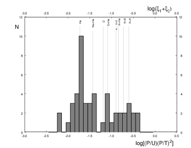
Figure 1: The distribution of binary stars on the value of $(\mathcal{P}/\mathcal{U})(\mathcal{P}/\mathcal{T})^{2}$.

All these data and references were given to us by Dr.K.F.Khaliullin (Sternberg Astronomical Institute) and are cited in [3]. On Fig.1 the lines mark the values of parameters (Eq.(13)) for different pairs of binary stars. It can be seen that the calculated values of the periastron rotation for stars composed by light elements which is summarized in Table 1 are in a good agreement with separate peaks of the measurement data distribution. It is important to underline that these results were obtained without using of any fitting parameters (and they are accurate in this regard). Reversely, the conventional approach to this problem based on Euler equation can not give any explanation for this measured distribution.

5 The solar seismical oscillations

5.1 The seismical oscillations at the Eulerian distribution of a substance

The measurements [4] show that the Sun surface is subjected to a seismic vibration. The most intensive oscillations have the period about five minutes and the wave length about $10^{4}$km or about hundredth part of the Sun radius. Their spectrum obtained by BISON collaboration is shown on Fig.2.

Figure 2: $(a)$ The power spectrum of solar oscillation obtained by means of Doppler velocity measurement in light integrated over the solar disk. The data were obtained from the BISON network [4]. $(b)$ An expanded view of a part of the frequency range.

These oscillations are a superposition of a big number of different modes of resonant acoustic vibrations. It is supposed that acoustic waves propagate on different trajectories in the interior of the Sun and have multiple reflection from surface. With these reflections trajectories of same waves can be closed and as a result standing waves are forming. Specific features of spherical body oscillations are described by the expansion in series on spherical functions. These oscillations can have a different number of wave lengths on the radius of a sphere ($n$) and a different number of wave lengths on its surface which is determined by the $l$-th spherical harmonic. It is accepted to describe the sunny surface oscillation spectrum as the expansion in series [5]:

$$\nu_{nlm}\simeq\Delta\nu_{0}(n+\frac{l}{2}+\epsilon_{0})-l(l+1)D_{0}+m\Delta\nu_{rot}.$$ (16)

Where the last item is describing the effect of the Sun rotation and is small. The main contribution is given by the first item which creates a large splitting in the spectrum (Fig.2)

$$\triangle\nu=\nu_{n+1,l}-\nu_{n,l}.$$ (17)

The small splitting of spectrum (Fig.2) depends on the difference

$$\delta\nu_{l}=\nu_{n,l}-\nu_{n-1,l+2}\approx(4l+6)D_{0}.$$ (18)

A satisfactory agreement of these estimations and measurement data can be obtained at [5]

$$\Delta\nu_{0}=120~{}\mu Hz,~{}\epsilon_{0}=1.2,~{}D_{0}=1.5~{}\mu Hz,~{}\Delta\nu_{rot}=1\mu Hz.$$ (19)

To obtain these values of parameters $\Delta\nu_{0},~{}\epsilon_{0}~{}D_{0}$ from theoretical models is not possible. There are a lot of qualitative and quantitative assumptions used at a model construction and a direct calculation of spectral frequencies transforms into a unresolved complicated problem.

5.2 The oscillation of the solar core at the GIEP effect

Fig.2 shows a central part of the whole spectrum of solar oscillations which was obtained at a very high frequency resolution. The whole spectrum of solar oscillations was obtained at a little worse resolution in the frame of the programm SOHO/GOLF [6], and it is shown in Fig.3 .

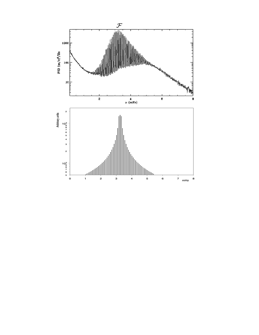
Figure 3: $(a)$ The spectrum of solar oscillations obtained by SOHO/GOLF group [6]. $(b)$ The theoretically obtained spectrum with using Eq.(25) at $Z=2$ $A/Z=5$.

The existence of this spectrum forces to change the view at all problems of solar oscillations. The theoretical explanation of this spectrum must give answers as minimum on four questions :

1.Why does the whole spectrum consist from a large number of equidistant spectral lines?

2.Why does the central frequency of this spectrum ${\cal F}$ is equal approximately to $\approx 3.23~{}mHz$?

3. Why does this spectrum splitting $f$ is equal approximately to $67.5~{}\mu Hz$?

4. Why does the intensity of spectral lines decrease from the central line to the periphery?

The answers to these questions can be obtained from the Sun core model based on the GIEP effect. According to this model, the Sun core has the high constant density (Eq.(11)) with radius ${\mathbb{R}}$, mass ${\mathbb{M}}$ at temperature ${\mathbb{T}}$, which all depend on $Z$ and $A/Z$ only [2].

5.2.1 The sound oscillation of the Sun core

Since the solar core is compressible, the main mode of its vibration should be elastic sound oscillations of its radius with the conserved spherical form of the core at the frequency $\Omega_{s}\approx V_{sound}/\mathbb{R}$. The detail calculation shows that the frequency of this mode [7]

$$\Omega_{s}=4.49\biggl{\{}\frac{10.5}{(3/2)^{7}\pi}\biggl{[}\frac{Gm_{p}}{r_{B}^{3}}\biggr{]}\biggl{\langle}\frac{A}{Z}\biggr{\rangle}\biggl{(}Z+1\biggr{)}^{3}\biggr{\}}^{1/2}.$$ (20)

is depending on a chemical composition of the core only. The same separate frequencies of this mode of the sound radial oscillation (${\cal F}=\Omega_{s}/2\pi$) for cores with the different $A/Z$ at $Z=1$ $Z=2$ are shown in the third column of Table 2.

		${\cal F},mHz$		${\cal F},mHz$
Z	A/Z		star
		(calculation Eq.(20))		measured
1	1	0.78	$\eta~{}Bootis$	0.85
			The Procion$(A\alpha~{}CMi)$	1.04
1	2	1.10
			$\beta~{}Hydrae$	1.08
2	2	2.02
	2.5	2.25
2			$\alpha~{}Cen~{}A$	2.37
	3	2.47
2	3.5	2.67
2	4	2.85
2	4.5	3.02
2	5	3.19	The Sun	3.23

Table 2.

The measured frequencies of the surface oscillations of separate stars [5] are shown in the right side of Table 2.

Comparing the calculated and measured frequencies, one can conclude that the Sun core must be composed in general by hellium-10. This conclusion doesn’t look so confusing because the pressure acting in core is running to $10^{18}~{}{dyn}/{cm^{2}}$ and it can induce the neutronization process in plasma [1] which makes neutron-excess nuclei stable. At this chemical composition we have

$${\cal F}=\frac{\Omega_{s}}{2\pi}=3.19~{}mHz.$$ (21)

The good agreement with the measurement data gives a possibility to argue that the central frequency of solar oscillation is related to the radial oscillations of its core.

5.2.2 ”Phonon-like”low frequency oscillations

Another mode of the solar core oscillations is related to the existence of the equilibrium core density $\eta$ (Eq.11). Any deviations of the density from this equilibrium value, for example which are caused by radial core oscillations, induce a mechanism of density oscillations around this equilibrium value with frequency [7]

$$\omega_{\eta}=\biggl{\{}\frac{\sqrt{\pi}~{}2^{4}}{\sqrt{10}~{}(3/2)^{7}}\alpha^{3/2}\biggl{[}\frac{Gm_{p}}{r_{B}^{3}}\biggr{]}\biggl{\langle}\frac{A}{Z}\biggr{\rangle}\biggl{[}Z+1\biggr{]}^{4.5}\bigg{\}}^{1/2},$$ (22)

It gives at $Z=2$ and $A/Z=5$:

$$f_{\eta}=\frac{\omega_{\eta}}{2\pi}=66.0~{}\mu Hz.$$ (23)

These oscillations of plasma are like phonons in solid bodies. The excitation of this mechanism can induce oscillations on multiple frequencies $k\omega_{\eta}$. Their intensity must be $k$ times weaker because a population of according levels in energetic distribution is reversely proportional to their energy $k\hbar\omega_{\eta}$. As a result these low frequency oscillations form spectrum

$$\sum_{k=1}\frac{1}{k}~{}sin(k\omega_{\eta}t)$$ (24)

If these low frequency oscillations $f_{\eta}$ are induced by the sound radial oscillation with frequency $\cal{F}$, they will modulate them. The radial displacements of the solar core surface form the spectrum

$$u_{R}\sim\sin~{}\Omega_{s}t\cdot\sum_{k=0}\frac{1}{k}~{}\sin~{}k\omega_{\eta}t~{}\approx\xi\sin~{}\Omega_{s}t+\sum_{k=1}\frac{1}{k}~{}\sin~{}(\Omega_{s}\pm k\omega_{\eta})t,$$ (25)

This calculated spectrum is shown on Fig.3b. It is can been seen from this figure that the model of the Sun based on GIEP effect gives a possibility to explain all basic details of the measured spectrum of oscillations and to obtain answers on all four questions which was formulated above. It is important to underline that the quantitative agreement between the calculated spectrum and the measurement data was obtained without using of any fitting parameters and only taking into account its chemical composition ($Z=2$ $A/Z=5$).

6 Another measurements which results are depending on a star interior construction

6.1 Stellar masses

The models of star interior based on the Euler equation does not give any possibilities to estimate values of star masses. The theory based on GIEP effect obtains a direct way for the star mass calculation [2]

$${\mathbb{M}}=1.5^{6}\biggl{(}\frac{10}{\pi^{3}}\biggr{)}^{1/2}\biggl{(}\frac{\hbar c}{Gm_{p}^{2}}\biggr{)}^{3/2}\biggl{\langle}\frac{Z}{A}\biggr{\rangle}^{2}m_{p}\\ \approx 6.47~{}M_{Ch}~{}\biggl{\langle}\frac{Z}{A}\biggr{\rangle}^{2},$$

Where $M_{Ch}=\biggl{(}\frac{\hbar c}{Gm_{p}^{2}}\biggr{)}^{3/2}m_{p}=3.71\cdot 10^{33}g$ is the Chandrasekhar mass.

The frequencies of natural oscillations of the Sun [7] show that the star core mass is approximately equal to 1/2 of the whole stellar mass. It gives us a way for the estimation of stellar masses and for the comparison with measurement results. The calculated values of star mass depend on one coefficient $A/Z$ only [2].

There is no way to determinate the core chemical composition of far stars, but some predications for it are possible. At first, there must be no stars which masses exceed the Sun mass more than one and a half orders, because it accords to limiting mass for stars consisting from hydrogen with $A/Z=1$. Secondly, though the neutronization process makes neutron-excess nuclei stable, there is no reason to suppose that stars with $A/Z>10$ (and with mass in hundred times less than hydrogen stars) can exist. Thus, GIEP-theory predicts that the whole mass spectrum must be placed in the interval from 0.25 up to approximately 25 solar masses. These predications are verified by measurements quite exactly. The mass distribution of binary stars is shown on Fig.4 [8]. (Using of this data is caused by the fact that only the measurement of parameters of the binary star rotation gives the possibility to determine their masses with satisfactory accuracy). Besides, one can see the presence of separate pikes for stars with $A/Z=3;4;5...$ and with $A/Z=3/2$ on Fig.4.

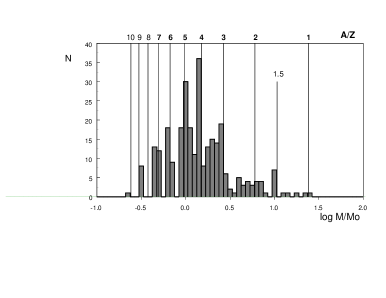
Figure 4: The mass distribution of binary stars [8]. On abscissa, the logarithm of the star mass over the Sun mass is shown. Solid lines mark masses agree with selected values of $A/Z$ from Eq.(6.1)

It is important to underline that the measured mass of the Sun is in a good agreement with the claim obtained above and stating that the Sun core must be basically composed by hellium-10. This two measurement - the mass measurement and the frequencies measurement - build a test practically for the whole GIEP-theory. The first one tests the formula of mass and the other checks formulas for the radius of the core and the sound velocity (i.e. the core density). The agreement of this measurement results confirms the reliability of the obtained formulas and of the whole approach.

6.2 The star magnetic fields

Another effect which follows from GIEP existence is the generation of a magnetic field by celestial bodies. These bodies, as they have electrically polarized cores, must induce magnetic moments due to their rotation:

$$\mu\approx\frac{Q_{bond}\Omega R^{2}}{c},$$ (26)

where $\Omega$ is the rotation velocity, $Q_{bond}=\frac{4\pi}{3}\rho_{bond}R^{3}$.

Figure 5: The observed values of the magnetic moments of celestial bodies vs. their angular momenta. On the ordinate, the logarithm of the magnetic moment over $Gs\cdot{cm^{3}}$ is plotted; on the abscissa the logarithm of the angular momentum over $erg\cdot{s}$ is shown. The solid line illustrates Eq.(28). The dash-dotted line is the fitting of the observed values.

Since the angular momentum of a star

$$L\approx M\Omega R^{2},$$ (27)

we can conclude that the giromagnetic ratios of celestial bodies must be directly expressed through world constants

$$\vartheta=\frac{\mu}{L}\sim\frac{\sqrt{G}}{c}$$ (28)

This theoretical predication can be checked by comparison with the measurement data. The values of giro-magnetic ratios for all celestial bodies (for which they are known today) are shown in Fig.5. The data for planets are taken from [9], the data for stars are taken from [10], and those for pulsars - from [11]. Therefore, for all celestial bodies - planets and their satellites, Ap-stars and several pulsars, which angular momenta distinguish within more than 20 orders - the calculated values of the gyromagnetic ratio (Eq.(28)) agree with measurements quite satisfactorily with the logarithmic accuracy.

7 Conclusion

First conclusion, which we obtain from the above analysis states that there are four distributions, obtained from measurements, which depend on properties of the substance inside stars and which must be explained theoretically. The astrophysical models which are based on the Euler equation can neither explain the dependence of the velocity of periastron rotation from a chemical composition (Fig.(1)), nor the star mass distribution (Fig.(4)), nor their giromagnetic ratios (Fig.(5)). In this way, the quantitative agreement can be obtained only by an individual fitting of model parameters. The explanation of the spectrum of the solar oscillations (Fig.(2)) by means of series expansion on spherical harmonics (Eq.(16)) can be considered as a fitting only because its parameters $\Delta\nu_{0},~{}\epsilon_{0}$ and $D_{0}$ are free and can not be obtained from the theory.

Quite the contrary, taking into account GIEP effect opens possibilities for the quantitative explanation with acceptable accuracy of all measured data without using any fitting parameters. A good agreement of the relatively simple formulas and the measurement data has the easy explanation: the cores of stars consisting of hot dense plasma are well described by the known ideal gas formulas with small corrections, which are also well determined by modern plasma physics.

References

- [1] Landau L.D. and Lifshits E.M. - Statistical Physics,1980, vol.1,3rd edition,Oxford:Pergamon.
- [2] Vasiliev B.V. - Nuovo Cimento B, 2001, v.116, pp.617-634.
- [3] Vasiliev B.V. - Astro-ph/0405297
- [4] Elsworth, Y. at al. - In Proc. GONG’94 Helio- and Astero-seismology from Earth and Space, eds. Ulrich,R.K., Rhodes Jr,E.J. and Däppen,W., Asrtonomical Society of the Pasific Conference Series, vol.76, San Fransisco,76, 51-54.
- [5] Christensen-Dalsgaard, J., - Stellar oscillation, Institut for Fysik og Astronomi, Aarhus Universitet, Denmark, 2003
- [6] Solar Physics, vol.175/2, (http://sohowww.estec.esa.nl/gallery/GOLF)
- [7] Vasiliev B.V. - Astro-ph/0409491
- [8] Heintz W.D. Double stars (Geoph. and Astroph. monographs. vol.15, D.Reidel Publ. Corp.) 1978.
- [9] Sirag S.-P. - Nature,1979,v.275,pp.535-538.
- [10] Borra E.F. and Landstreet J.D. (1980) 421.
- [11] Beskin V.S., Gurevich A.V., Istomin Ya.N. Physics of the Pulsar Magnetosphere (Cambridge University Press) 1993.