Nonlinear Evolutions and Non-Gaussianity in Generalized Gravity
Abstract
We use the Hamilton-Jacobi theory to study the nonlinear evolutions of inhomogeneous spacetimes during inflation in generalized gravity. We find the exact solutions to the lowest order Hamilton-Jacobi equation for special scalar potentials and introduce an approximation method for general potentials. The conserved quantity invariant under a change of timelike hypersurfaces proves useful in dealing with gravitational perturbations. In the long-wavelength approximation, we find a conserved quantity related to the new canonical variable that makes the Hamiltonian density vanish, and calculate the non-Gaussianity in generalized gravity. The slow-roll inflation models with a single scalar field in generalized gravity predict too small non-Gaussianity to be detected by future CMB experiments.
pacs:
98.80.Cq, 04.50.+hI Introduction
Inflation scenario is a successful model to solve the problems of the standard Big Bang theory and explains remarkably the observational data. Quantum fluctuations of a scalar field are adiabatic and Gaussian during the inflation period and provide a seed for density perturbations. The amplitudes of the perturbations freeze out when the perturbations stretch out to the superhorizon scale by an accelerated expansion. Inflation also gives the scale invariant spectrum () when the perturbation modes cross the horizon. Linear perturbation theory is enough to explain these gravitational perturbations and temperature anisotropy in the early universe.
Recent WMAP observations komatsu03 try to find a signal of the non-Gaussianity in the temperature anisotropy. The non-Gaussian signal in the CMB anisotropy might be generated either from the non-vacuum initial state gangui02 or from nonlinear gravitational perturbation acquaviva03 . Gaussian statistical properties are completely specified by the two-point correlation function. However, the two-point correlation function is not sufficient to describe the statistical properties of the non-Gaussianity, so it is necessary to investigate higher order correlations such as the three-point correlation for nonlinearity of a perturbation field or the four-point correlation for a non-vacuum initial state. Second order perturbation theory has been used to explain the non-Gaussianity in the temperature anisotropy acquaviva03 . In addition to second order perturbation theory, the Hamiltonian formalism turned out to useful to deal with nonlinear evolutions in the early universe and was applied to canonical quantum gravity dewitt67 or semiclassical gravity banks85 ; kim92 for a long time.
Salopek and Bond in Ref. salopek90 employed the Hamiltonian formalism to study the nonlinear evolutions of gravitational perturbations. It was also applied to Brans-Dicke theory soda95 and low energy effective string theory saygili99 . Especially, the Hamilton-Jacobi theory provides a powerful tool to get solutions of nonlinear evolutions in the early universe through a generating functional which satisfies the momentum constraint equation. Even though it is difficult to get exact solutions of the Hamilton-Jacobi equation for general potentials, the large scale perturbation, which contributes mainly to the large scale structure in the present Universe, could be treated appropriately using the long wavelength approximation. The long wavelength approximation assumes that the length scale of the spatial variation is much longer than the Hubble radius, so it is a reasonable assumption to deal with super-horizon scale perturbations. It is also known that the gauge invariant conserved quantity exists in nonlinear perturbation theory for a superhorizon scale salopek90 ; rigopoulos03 ; lyth04 .
Brans-Dicke type gravity naturally emerges from the fundamental theory of particle physics such as string or M-theory. Although it is not clear how scalar fields couple to gravity, it is necessary to investigate the perturbations in the alternative gravity theory such as type gravity as well as in Einstein gravity. Recent supernovae observation perlmutter99 and WMAP results spergel03 imply that our universe today is in an accelerated expansion phase and dominated by the dark energy which has the equation of state, . It is also needed to consider nonlinear evolutions of such a matter component to see whether their existence affects the temperature anisotropy.
In this paper, the Hamilton-Jacobi formalism will be used to study the nonlinear evolutions of inhomogeneous spacetimes in generalized gravity theory during the inflation period. The canonical variables will be transformed to new ones that make the new Hamiltonian density vanish and these new variables are constant in time for fixed spacelike hypersurfaces. The gauge invariant quantity, , which is conserved in the large scale limit, is derived from one of new canonical variables. By introducing the nonlinear parameter, , the conserved quantity may be decomposed into a linear Gaussian part, , and a nonlinear part komatsu01 :
| (1) |
Non-Gaussianity is parameterized through which will be constrained by observations. It is generally expected to be difficult to detect a non-Gaussian signal in CMB experiments for a single field inflation model in Einstein gravity acquaviva03 . So the detection of the non-Gaussianity can constrain different inflation models.
This paper is organized as follows. In Sec. II, we derive the Hamilton and momentum constraint equations in generalized gravity. The Hamilton-Jacobi equation will be obtained through a canonical transformation. Assuming a generating functional which satisfies the momentum constraint equation, we get the conserved quantity that is invariant under a change of timelike hypersurfaces in the long-wavelength approximation. In Sec. III, non-Gaussianity will be computed using the generalized curvature perturbation on comoving hypersurfaces. Finally, we discuss the physical implications of the non-Gaussianity in generalized gravity in Sec. IV.
II Hamilton-Jacobi Formalism in Generalized Gravity
II.1 Hamilton equations
The generalized gravity action to be studied in this paper is given by
| (2) |
where and are functions of a scalar field . We shall confine our attention to the slow-roll inflation models that are described by this action. Einstein gravity is recovered when and . Further, Brans-Dicke theory is prescribed by and ; the non-minimally coupled scalar field theory corresponds to and ; the low energy effective string theory is given by and . We consider the Arnowitt-Deser-Misner (ADM) metric
| (3) |
where and are a lapse function and a shift vector, respectively, and is a 3-spatial metric. The -dimensional Ricci scalar, , can be written in terms of the 3-dimensional Ricci scalar, , and the extrinsic curvature, , as mtw73
| (4) |
The terms in the square bracket in the above formula are total derivatives or surface terms so that they can be integrated out in Einstein gravity. They cannot, however, be neglected in generalized gravity. The extrinsic curvature tensor and trace are given by
| (5) |
where the vertical bar is a covariant derivative with respect to . The is a generalization of the Hubble parameter. By varying action with respect to and , the momenta conjugate to and are obtained as
| (6) | |||||
| (7) |
From these relations, can be written as
| (8) |
where . Variations of the action with respect to and lead to the Hamiltonian and momentum constraint equations, respectively,
| (9) | |||||
| (10) |
where
| (11) |
Then one finds the action of the form
| (12) |
Here, and are considered as Lagrange multipliers. The evolution equations for and can be obtained by varying the action (12) with respect to and :
| (13) | |||
| (14) |
II.2 Hamilton-Jacobi equation
To solve the Hamiltonian and the momentum constraint equations, (9) and (10), we use the Hamilton-Jacobi theory. Through an appropriate canonical transformation from and to new ones and , we can construct a vanishing Hamiltonian
| (15) |
where
| (16) |
and the generating functional is a function of and . Then the canonical transformation gives the following relations
| (17) |
Finally, we get the Hamilton-Jacobi equation from the Hamiltonian constraint
| (18) |
and the momentum constraint equation
| (19) |
The momentum constraint equation implies that the generating functional is invariant under spatial coordinate transformations. In general, the momentum constraint equation does not vanish through canonical transformations as long as does not vanish. On the contrary, the Hamiltonian constraint vanishes strongly. It is difficult to solve the Hamilton-Jacobi equation, (18), in general, except for special cases such as an exponential potential in Einstein gravity salopek90 .
II.3 long-wavelength approximation
To deal with the large scale gravitational perturbations, it is reasonable to use the approximation that temporal variations of fields are much greater than spatial variations. In inflation scenario, the inhomogeneous field, whose physical wavelength is much larger than the horizon size at the end of the inflation period, mostly contributes to formation of the large scale structure in the present universe and large angle CMB anisotropy. The long wavelength approximation assumes that the characteristic scale, , of spatial variations is much longer than the Hubble radius, , salopek90 ; soda95 :
| (20) |
where is a Hubble parameter, and and are a physical and a comoving wavelength, respectively. The generating functional can be expanded in a series of spatial gradient terms
| (21) |
The lowest order Hamilton-Jacobi equation neglects the terms containing spatial gradients. In this paper we only consider the lowest order Hamilton-Jacobi equation which is sufficient for dealing with the nonlinear evolution of the inhomogeneous gravitational fields. Then the lowest order Hamilton-Jacobi equation is
| (22) |
We assume that the lowest order generating functional takes the following form
| (23) |
where is a new canonical variable involving and , and is a constant which carries a dimension. For Einstein gravity, can be interpreted as a locally defined Hubble parameter if we take salopek90 . This generating functional automatically satisfies the momentum constraint equations if , and this will be discussed in the next section.
It is convenient to factor the 3-spatial metric into a conformal factor and a conformal 3-spatial metric with the unit determinant :
| (24) |
The gravitational waves are related to the . Then, from Eq. (17), the conjugate momenta for and are
| (25) | |||||
| (26) |
where we have used salopek91
| (27) |
which is traceless, . If we decompose into the trace and the traceless part , they are given by
| (28) |
As long as we do not concern about the gravitational radiations, is assumed to be independent of , so can be set to zero. Then the Hamilton-Jacobi equation becomes
| (29) |
and the evolution equations for and are
| (30) | |||||
| (31) |
II.4 Solutions of Hamilton-Jacobi equation
Although the Hamilton-Jacobi equation (29) is difficult to be exactly solved for general potentials, it can be solved for some special cases in generalized gravity.
II.4.1
If the potential is given by , then the Hamilton-Jacobi equation takes the form
| (32) |
where
| (33) |
As , Eq. (32) can be exactly integrated to yield handbook
| (34) |
where is an integration constant. The solution of the form (34) is available for a constant potential in Einstein gravity or a massive scalar field potential for the generalized gravity with .
II.4.2 or general potentials
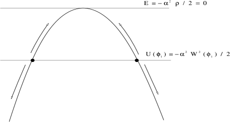
With the identification of and , the Hamilton-Jacobi equation may be interpreted as a time-dependent inverted oscillator with a unit mass, frequency , and energy :
| (35) |
where . In fact, this inverted oscillator has a -dependent energy and curvature (spring constant) of potential. The are two fixed or stationary points.
First, in the case of corresponding to the Brans-Dicke gravity or low energy effective string theory, the solution can easily be obtained
| (36) |
where is an initial value at . When is non-square integrable, the solution (36) for the upper sign grows to as goes to depending on the sign of . This corresponds to the downward motions in Fig. 1. Whereas, for the lower sign, the solution approaches an attractor 0 regardless of as goes to . The solution approaches the attractor 0 regardless of for the upper sign, but it diverges to for the lower sign depending on the sign of as goes to . On the other hand, for a square integrable , as goes to , the solution (36) approaches finite values, , not necessarily attractors, which correspond to the upward motions in Fig. 1.
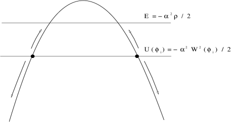
For general potentials with , we have a similar picture as shown in Fig. 2. Not only the energy but also the curvature of the potential depend on . In the analogy of an oscillator, as shown in Fig. 2, the total energy line moves up or down depending on and the -dependent curvature narrows or widens the parabola. As for the case, either approaches to attractors or diverges to , depending on the sign of and the behavior of and , as grows. This behavior of for general potentials can be calculated numerically koh05 .
To find approximately an analytical solution for general potentials, we can write as , where is a homogeneous solution (36). Then the Hamilton-Jacobi equation reduces to the equation for :
| (37) |
where we have used Eq. (35) for . Equation (37) is a nonlinear equation for . Assuming that is a slowly varying function of , we can introduce a small parameter to indicate smallness of the nonlinear terms and rewrite Eq. (37) as
| (38) |
The parameter will be set to one in the final result. Now we expand in a series of
| (39) |
Substituting Eq. (39) into Eq. (38) and comparing terms of the same powers of , we obtain the following equations up to first order
-
•
:
(40) -
•
:
(41)
The solutions at each order can easily be found
| (42) |
On the other hand, for a rapidly varying function , we can repeat the same analysis and write Eq. (37) as
| (43) |
With the series expansion (39) for , we obtain the following equations up to first order
-
•
:
(44) -
•
:
(45)
These equations can be simply integrated to give
| (46) |
The validity of the approximation in Eqs. (38) and (43) for specific models will be discussed in a future work koh05 .
II.5 conserved quantities
In Eq. (23), depends on , , and , where is a new canonical variable that has the conjugate momentum
| (47) |
Then the momentum constraint equation (10) reduces to salopek91
| (48) |
Since the new variable is chosen to make the new Hamiltonian density vanish, the new Hamiltonian contains only a contribution from the momentum constraint
| (49) |
The Hamilton equations for the new variable are
| (50) |
In general, the new canonical variable needs not to be constant in time, but if the spacelike hypersurfaces are chosen such that the shift vector, , vanishes, then and are constants for fixed spatial coordinates salopek91 .
It is known that a gauge invariant quantity can be derived by taking the spatial gradient of an inhomogeneous quantity ellis89 ; rigopoulos03 . By taking the spatial gradient of the logarithm of the canonical new variable (47), we can obtain the gauge invariant quantity
| (51) |
To calculate the last term in the above equation, we differentiated the Hamilton-Jacobi equation (29) with respect to :
| (52) |
With this relation, Eq. (51) now becomes
| (53) |
where we have used Eqs. (30) and (31). This quantity is similar to the gauge invariant quantity in the linear perturbation theory, which is conserved at the superhorizon scale. Here is a Newtonian gravitational potential. We define the generalized gauge invariant quantity in nonlinear theory, which is conserved in the large scale limit
| (54) |
Although is defined on the uniform energy density hypersurfaces in general, it coincides with a curvature perturbation , which is defined on the comoving hypersurfaces in a scalar field dominated universe and also conserved in the large scale limit. and are proved to be conserved in the large scale limit in Refs. rigopoulos03 ; lyth04 .
III Non-Gaussianity in generalized gravity
Non-Gaussianity in CMB might be generated by a non-vacuum initial state gangui02 or a nonlinear perturbation acquaviva03 , even though the initial perturbation is Gaussian. Although the non-vacuum initial state gives the zero three-point correlation function, the relation between the four-point and the two-point correlation functions, which obey the Gaussian statistics,
| (55) |
is no longer satisfied gangui02 . Whereas the nonlinear gravitational perturbation leads to a non-zero three-point correlation function. In this paper we shall focus on the non-Gaussian signal in CMB only from nonlinear perturbations. To show the non-Gaussianity by the nonlinear perturbation, the gravitational potential may be decomposed into a linear part and a nonlinear part with a nonlinear parameter komatsu01
| (56) |
Here, is a linear Gaussian perturbation that has the zero expectation value .
With this definition, the non-vanishing component of the -bispectrum, which is the Fourier transform of the three-point correlation function in the coordinate space, is komatsu01
| (57) |
where is the linear power spectrum given by
| (58) |
and
| (59) |
It is known that should be larger than order unity to be detectable by CMB experiment. But the single field inflationary model gives too much small value of where and are slow-roll parameters acquaviva03 . Thus, if the non-Gaussianity is detected, it can constrain inflationary models. However, it would be interesting to calculate non-Gaussianity in generalized gravity theories.
We follow the method in Ref. salopek90 to calculate the nonlinear curvature perturbations on the comoving hypersurfaces. The 3-spatial metric can be written as
| (60) |
where is a local expansion factor, and the conformal 3-metric, , is independent of time and has the unit determinant, . Then the local Hubble parameter takes the form
| (61) |
If we choose as a time coordinate on the comoving hypersurfaces, we can obtain from Eq. (30)
| (62) |
We use the notation for the scalar field fluctuation on the spatially flat hypersurfaces and for the curvature perturbation on the comoving hypersurfaces . The scalar field fluctuations on the spatially flat hypersurfaces are needed to transform to the curvature perturbation on the comoving hypersurface. Then the curvature perturbation on comoving hypersurfaces is given by
| (63) |
Using Eqs. (30) and (31), we get
| (64) |
where
| (65) |
By expanding the nonlinear relation between and up to second order komatsu02 , we obtain a nonlinear curvature perturbation, , where
| (66) | |||||
| (67) |
where
| (68) |
Finally, from Eq. (56), we obtain the nonlinear parameter
| (69) |
where we have used the relation between and as during the matter dominated era. If we define the slow-roll parameters in generalized gravity theories by
| (70) | |||||
| (71) |
using again Eqs. (30) and (31), we obtain
| (72) | |||||
| (73) | |||||
The nonlinear part of the curvature perturbation can be written in terms of the slow-roll parameters, and , as
| (74) |
Hence, the nonlinear parameter, , for generalized gravity theories takes the form
| (75) |
Note that the nonlinear parameter (75) in generalized gravities has the same form as in Einstein gravity. The WMAP result gives a constraint on by at CL komatsu03 . Since the slow-roll inflation implies that , non-Gaussianity in the single scalar field inflation model is difficult to be observed by CMB experiments.
IV Conclusion
It is expected that nonlinear perturbations may be responsible for a non-Gaussian signal in CMB experiments. The Hamilton-Jacobi theory can provide a useful and convenient tool to deal with nonlinear perturbations. In this paper we derived the Hamilton-Jacobi equation in generalized gravity theory. Through a canonical transformation, a new set of canonical variables was chosen that could make the new Hamiltonian density vanish. The conserved quantity, , was obtained in the large scale limit by using the fact that the new canonical variable is constant in time on fixed spacelike hypersurfaces. The could be regarded as a generalization of the gauge invariant quantity in the linear perturbation theory. In the long wavelength approximation, we found the exact solutions to the lowest order Hamilton-Jacobi equation for special scalar potentials and introduced an approximation scheme for general potentials.
The non-Gaussianity from nonlinear density perturbations was parameterized with a nonlinear parameter , which is an expansion parameter of the gravitational potential in Eq. (56). The nonlinear parameter can be measured by CMB observations. Any detection of the non-Gaussianity of CMB may put a strong constraint on inflation models. Especially, predicted by the single field slow-roll inflation in Einstein gravity is too small to be detected in CMB experiments through a non-Gaussian signal. Nevertheless, it would be interesting to investigate the non-Gaussianity in generalized gravity theory. We have found that even in generalized gravity theory, the nonlinear parameter for the slow-roll inflation takes the same form as in Einstein gravity. Hence, the slow-roll inflation models based on Brans-Dicke theory, non-minimally coupled scalar field theory, and low energy effective string theory, et al as well as Einstein gravity will have the same order of non-Gaussianity for CMB. This has a physical implication that slow-roll inflation models with a single scalar field in such alternative theories of gravity will be ruled out if a signal for non-Gaussianity is observed in future CMB experiments. Therefore, the non-Gaussianity would require multi-field inflation models or a different generating mechanism for density perturbations bartolo04 in generalized gravity.
Acknowledgements.
This work was supported by Korea Astronomy Observatory (KAO).References
- (1) E. Komatsu, et al., Astrophs. J. Suppl. 148, 119 (2003).
- (2) J. Lesgourgues, D. Polarski, and A. A. Starobinsky, Nucl. Phys. B497, 479; A. Gangui, J. Martin, and M. Sakellariadou, Phys. Rev. D 66, 083502 (2002).
- (3) V. Acquaviva, N. Bartolo, S. Matarrese, and A. Riotto, Nucl. Phys. B 667, 119 (2003); J. Maldacena, J. High Energy Phys. 05, 013 (2003).
- (4) B. DeWitt, Phys. Rev. 160, 1113 (1967).
- (5) T. Banks, Nucl. Phys. B249, 332 (1985); C. Kiefer, Class. Quantum Grav. 4, 1369 (1987); C. Kiefer and T. P. Singh, Phys. Rev. D 44 1067 (1991).
- (6) S. P. Kim, Phys. Rev. D 52, 3382 (1995); ibid. 55, 7511 (1997).
- (7) D. S. Salopek and J. R. Bond, Phys. Rev. D 42, 3936 (1990).
- (8) J. Soda, H. Ishihara, and O. Iguchi, Prog. Theor. Phys. 94, 781 (1995).
- (9) K. Saygili, Int. J. Mod. Phys. A 14, 225 (1999); P. Kuusk and M. Saal, Gen. Rel. Grav. 34, 353 (2002).
- (10) G. I. Rigopoulos and E. P. S. Shellard, Phys. Rev. D 68, 123518 (2003).
- (11) E. W. Kolb, S. Matarrese, A. Notari, and A. Riotto, astro-ph/0410541; D. Lyth and K. Malik, astro-ph/0411220 (2004); F. Vernizzi, astro-ph/0411463 (2004).
- (12) S. Perlmutter et al., Astrophys. J. 517, 565 (1999).
- (13) D. Spergel et al., Astrophys. J. Suppl. 148, 175 (2003).
- (14) E. Komatsu and D. Spergel, Phys. Rev. D 63, 063002 (2001).
- (15) C. W. Misner, K. S. Thorne, and J. A. Wheeler, Gravitation, (W.H. Freeman, 1973).
- (16) D. S. Salopek, Phys. Rev. D 43, 3214 (1991).
- (17) A. D. Polyanin and V. F. Zaitsev, Handbook of Exact Solutions for Ordinary Differential Equations, (CRC Press, New York, 1995).
- (18) S. Koh, S. P. Kim, and D. J. Song, in preparation.
- (19) G. F. R. Ellis and M. Bruni, Phys. Rev. D 40, 1804 (1989).
- (20) E. Komatsu, Ph. D thesis, astro-ph/0206039.
- (21) N. Bartolo, E. Komatsu, S. Matarrese, and A. Riotto, astro-ph/0406398 (2004).