GLOBAL STAR FORMATION FROM ${\bf z=5\times 10^{-8}}$ to ${\bf z=20}$

Starting with the assertion that the problem of isolated, single star formation is essentially solved, this paper examines some of the missing steps needed to go from there to understanding the star formation history of the Universe. Along the way, some results on the formation of star clusters in the Milky Way and the properties of GMCs in nearby galaxies are briefly examined.

Keywords: Stars: formation; ISM: general; Galaxies: evolution

1 Introduction

The field of star formation exploded with the advent of millimeter-wave and infrared detectors in the 1970s. Prior to that it was a field with a few lonely but brilliant workers such as George Herbig and Adriaan Blaauw who managed to identify young stars and regions of star formation from their optically determined properties alone. Both realized that the regions of most recent star formation were always associated with dark dust clouds, and understood that the earliest stages of star formation would only be probed by penetrating the veil of dust obscuration. Since that time, the field of star formation has expanded to include not just the nearest accessible regions, but the farthest reaches of the Universe as well. Using what we’ve learned about local star formation, reasonable speculations and simulations have now been attempted to guess at what the first stars in the Universe might have been like (Abel, Bryan & Norman 2002) $\!{}^{{\bf?}}$.

The field of star formation remains a rich area of research with many unsolved problems and thus continues to attract a coterie of young inventive scientists. In this article I give a personal view of where some parts of the field are headed, especially those areas that touch on star formation in galaxies. Clearly, in such a short space, I can cover only a few topics, and even those, rather cursorily.

2 What Do We Really Want to Know?

I begin by making the outrageous claim that the problem of low-mass, single star formation is essentially solved, due in large part to the work of Frank Shu, Richard Larson and a number of others. This is not to say that there aren’t still questions that are worth asking, but that the most interesting questions are more in the realm of planet formation than star formation. The remaining star formation issues are questions more of detail, rather than questions of a fundamental nature about how stars form. I illustrate this point with reference to what I believe is the most well known image in the scientific literature on the subject of star formation, which is shown here as Figure 1 (Shu, Adams & Lizano 1987) $\!{}^{{\bf?}}$. (Jeff Hester’s beautiful image of the elephant trunk structures in the Eagle Nebula is more well known, but is reproduced primarily in the popular press).

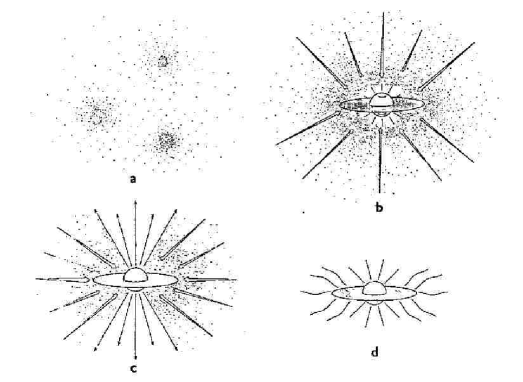
Figure 1: Figure taken from the 1987 review of low-mass star formation by Shu, Adams, and Lizano, giving the four principle stages of star formation. Although there has been some refinement of these stages, there is general agreement among astronomers that star and solar system formation occur according to this picture, which allows detailed quantitative estimates to be made to compare with observations.

This sketch represents the four stages of star formation which are now generally accepted as how low-mass, single stars form. Stars begin as gravitationally unstable condensations in cold, dense molecular clouds, forming a prestellar core observable in the near infrared as material continues to rain in on it. The higher angular momentum material forms a disk, and the system develops a bipolar outflow and jet which removes the angular momentum from the system, while initially disrupting and clearing out the infalling material. The star becomes visible as a T-Tauri star, and the disk ultimately becomes the raw material from which planets form. Magnetic fields play a central role in the dynamics, and add computational complexity, but almost surely determine the onset of collapse and the bipolar outflows. Diverse observations have a good theoretical underpinning, and little work is now done without either explicitly or implicitly invoking this picture.

On the other end of the distance scale, deep observations with the HST, Keck and SCUBA, have made it possible to determine the star formation history of the Universe, which is shown in Figure 2 (Steidel et al. 1999) $\!{}^{{\bf?}}$. This plot, widely known as the Madau plot (Madau et al. 1996) $\!{}^{{\bf?}}$, has been modified by others (e.g. Rowan-Robinson 2002 $\!{}^{{\bf?}}$), but its main features are well established: at early times there is a constant, or nearly constant star formation rate per comoving Mpc until about $z$ = 2, at which time the star formation rate steadily falls by about an order of magnitude until the present epoch. One of the great challenges is to apply what we know about the details of star formation in the nearest regions to fill in the missing pieces needed to obtain Figure 2. The goal is to obtain not only the correct shape, but the correct amplitude of the Madau function.

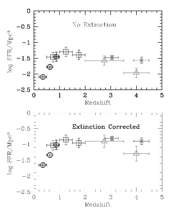
Figure 2: The star formation rate in the universe as a function of redshift. The units on the ordinate are M_⊙ Mpc^-3 yr^-1 based on the work of (Steidel et al. 1999).

2.1 Some of the Missing Pieces

High Mass Star Formation

The first problem is that the star formation rate in the Universe is determined from the light of the most massive stars, but most of what we know about star formation applies only to low mass stars. Getting an evolutionary picture of high mass star formation remains difficult observationally because of the rapid destruction of their surroundings by high mass protostars. Without a good set of observations it is difficult to make progress in the theory. For example, only a small number of candidate high mass prestellar cores have been identified, and little has been written about the relationship of these cores to their surrounding molecular clouds. Nevertheless, considerable progress should be possible in the near term from observations with a new generation of millimeter-wave interferometers: CARMA and ALMA, the Spitzer Space Telescope, and SOFIA.

The Formation of Stars in Clusters

If the problem of how individual low-mass stars form is essentially solved, and if high-mass star formation is next, we only get to the first rung of the ladder that ends at the Madau plot. Stars do not typically form as isolated objects, but rather in clusters, and little is known about clustered star formation. For example, do massive clumps form massive star clusters? What determines the star formation efficiency of a particular cluster forming clump? Are the stars that form in a cluster different from those that form in looser aggregates? Are the prestellar cores that form star clusters in the gas clumps the same as those identified with single star formation?

The study of clustered star formation is in such a primitive state that even some of the most basic questions have not yet been addressed. For example, it would seem that high mass stars are the last to form in clusters (lest they dissociate the gas from which the accompanying low mass stars form), and they appear to form in the cluster centers. But how can this be the case since high mass protostars should have the shortest dynamical times, and if formed in the centers of the clumps, should form first since the density of the gas is highest there. Although there have been several guesses at a solution (e.g. Stahler, Palla & Ho 2000 $\!{}^{{\bf?}}$; Bonnell, Bate & Zinnecker 1998 $\!{}^{{\bf?}}$), no explanation seems compelling yet.

Universality of the IMF

The calibration of the vertical scale in Figure 2 assumes that the IMF is invariant at all epochs and in all galaxies. But how universal is the IMF? To predict how it might or might not vary in other galaxies, and at other epochs, we need to know what physical or stochastic processes determine it. Very little is known about how the initial mass function is produced, though new work by Shu, Li, & Allen (2004) $\!{}^{{\bf?}}$ promises some progress on that subject.

The Formation of Stars in Galaxies

It may be a long time before it is possible to understand enough about the details of star formation to predict how star formation proceeds on galactic scales in GMCs. Nevertheless, it may be possible to circumvent this issue by learning how GMCs form and then determining how star formation proceeds on average in these GMCs. With this approach one would need to know how the physical conditions in GMCs differ in various galaxy types, in different locations within a galaxy, and with changes in metallicity. While this may seem like a daunting task, improvements in instrumentation now make it possible to survey entire galaxies at high enough resolution to make significant progress. Some early results are discussed below.

The last step in getting to the Madau plot is then extrapolating what we know about global star formation in normal galaxies to the star formation in starbursts and AGN. In other words, why do particular galaxies become starbursts, and how much star formation comes from particular galaxy or merger? This step is important because a significant fraction of the light of galaxies comes from starbursts, and the fraction of starbursts seems to change with $z$.

Initial conditions, Initial Conditions, Initial conditions

What ties all of these points together is that to make the step from single star formation to the Madau plot, it is necessary not only to learn about the physical processes involved, which requires a combination of theory and observation, but to understand what the initial conditions are that give rise to variations in each step. For example, even if the process of isolated single star formation is essentially solved, we really have no idea how the intial conditions, the star forming cores, are produced. Furthermore, we don’t know whether the IMF reflects the mass spectrum of prestellar cores as suggested by Motte, Andre & Neri (1998) $\!{}^{{\bf?}}$ and Testi & Sargent(1998) $\!{}^{{\bf?}}$, or the process of star formation itself (Shu, Li, & Allen 2004 $\!{}^{{\bf?}}$). The beautiful work by Alves, Lada & Lada (2001) $\!{}^{{\bf?}}$ suggests that the initial configuration for star formation may be better represented by a Bonner-Ebert sphere rather than a singular isothermal sphere (Shu 1977) $\!{}^{{\bf?}}$. Does this make a significant difference in the star that is produced? What are the initial conditions in a GMC that produce the difference between relatively isolated star formation (as in Taurus) and clustered star formation (as in Orion)? What are the initial conditions that give rise to the number and distribution of GMCs in a galaxy?

My own view is that we cannot know too much about typical initial conditions and how they vary. Therefore, there cannot be too much emphasis on trying to determine what the intial conditions are for forming individual low mass and high mass stars, for forming stars in clusters (why, for example, do some become globular clusters?), and for forming GMCs in the disks and centers of normal and starburst galaxies.

3 A Few Relevant Results

3.1 Beyond Single Star Formation

One of the first attemps to study to study the formation of star clusters observationally was done by Elizabeth Lada (Lada 1992) $\!{}^{{\bf?}}$, who made the first survey of dense gas in an entire GMC (Orion B) using the molecular tracer CS. She found that the embedded stars are found primarily in clusters, and that the clusters form only in the densest condensations: those identified by their CS emission. Subsequently, Phelps & Lada (1997) $\!{}^{{\bf?}}$ made another advance with their near IR imaging of some of the ¹³CO clumps in the Rosette Molecular Cloud. They were able to identify 7 embedded clusters associated with the centers of 7 massive clumps of molecular gas identified previously by Williams, Blitz & Stark (1995) $\!{}^{{\bf?}}$. These 7 clusters were all associated with far IR IRAS sources, and 5 were previously unknown. Thus what appeared to be single point sources in the IRAS data turned out to be embedded star clusters. Figure 3 shows a plot of the clumps in the Rosette vs. the gravitational boundedness of the clumps, plotted as $M_{grav}/M_{lum}$ where $M_{grav}=RV^{2}/G,~{}M_{lum}=X\int\int\int T_{A}dvdxdy$ and $X$ is the usual CO-to-H₂ conversion factor.

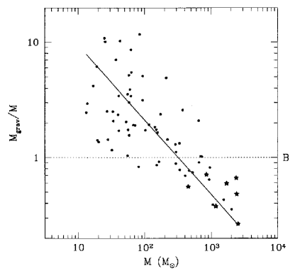
Figure 3: Plot of the ratio of gravitational binding energy to kinetic energy of the clumps in the Rosette Molecular Cloud from Williams, et al.(1995). The horizontal line represents a clump that is marginally self gravitating; clumps that are not self-gravitating are presumably pressure bound. The clumps containing IRAS sources are shown with stars. These are largely coincident with the embedded dlusters found in the infrared by Phelps & Lada (1997).

The clusters identified by Phelps & Lada $\!{}^{{\bf?}}$ are identified with the most massive, gravitationally bound clumps (Williams et al., 1995) $\!{}^{{\bf?}}$. But what is it about the star-forming clumps that produces a great many star-forming cores simultaneously? In other words, what is it that is communicated through a clump in a crossing time to let all parts know that they must produce stars simultaneously? What determines how many stars form within a given clump? Do the clumps even have embedded cores that are distinct, recognizable entities? The Phelps & Lada work also provides an efficient way to find embedded clusters, and, en passant, demonstrates that the clumps are real, long-lived entities, rather than ephemeral turbulent structures, as some authors have suggested (otherwise the star clusters would not have had enough time to form in them).

3.2 Star Formation on Galactic Scales

Understanding clustered star formation will likely solve the problem of how star formation takes place within an individual molecular cloud. How then do we extrapolate to larger scales, to the scale of an entire galaxy? A reasonable question to ask is whether we need to know all of the details of the star formation process to address star formation on galactic scales. That is, since we know that star formation takes place only in molecular clouds, and that the star formation efficiency in molecular clouds tends to be small ($\sim 5\%$), with relatively little variation in normal galaxies, perhaps the question of how stars form in galaxies reduces to a question of how the molecular clouds themselves form? That is, if we can understand how the ISM turns molecular gas into GMCs, and we can understand how the different conditions within GMCs translate into different star formation efficiencies and perhaps even IMFs, then it should be possible to determine the global star formation rate from just the gas content and other physical conditions within the galaxies.

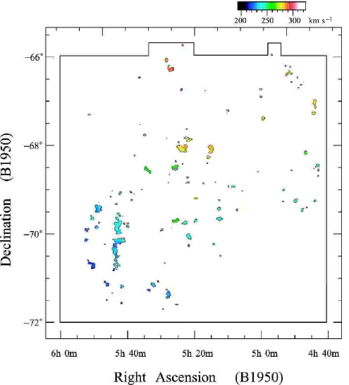
Figure 4: Map of the GMCs found in the LMC by Mizuno et al. (2001). These cover essentially the entire face of the galaxy, but cover only a small fraction of the surface, necessitating a large effort to obtain the map.

To this end, it is useful to have complete surveys of individual GMCs in entire galaxies not just unresolved images of the molecular gas, This has become possible only in the last few years, but for only a few galaxies; only two such maps have been published. The first was the LMC which has been nearly completely mapped by Mizuno et al. (2001) $\!{}^{{\bf?}}$ using the 4m Nanten telescope (see Figure 4). More recently, Engargiola et al. (2003) $\!{}^{{\bf?}}$ have used the BIMA array to make a 759 field mosaic of M33 at 15^′′ resolution ($\sim 50$ pc – see Figure 5). Both of these images indicate the difficulty in surveying galaxies for individual GMCs: the surface filling fraction of GMCs in galactic disks is small (see Figure 4), and the resolution needed to determine the cloud properties is high, requiring either large amounts of telescope time for Local Group objects, or high sensitivity interferometric mosaics for galaxies farther away. For both the LMC and M33, followup observations at high resolution were needed to resolve the molecular clouds in each case.

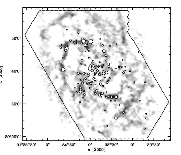
Figure 5: The molecular clouds catalogued by Engargiola et al. (2003), shown as white dots enclosed by black circles, superimposed on an HI map from the data of Deul and van der Hulst (1987). The area of each dot is proportional to the H₂ mass of each GMC. Notice both the filamentary structure of the HI and the good correspondence between the filaments and the location of the GMCs.

Other galaxies that have been fully mapped to date but not yet published include the SMC (Mizuno et al.), IC10 (Leroy et al.), and M31 (Muller and Guelin); these maps were all presented at this YLU conference. Although there has been a herculean effort to map the molecular gas in M31, the resolution (90 pc) appears to be too low to resolve clouds blended in the beam in many directions (Muller, this conference). Followup interferometric observations will be needed to obtain the properties of the GMCs. The central region of M64 has also been mapped at high enough resolution to measure the molecular cloud properties in the nuclear region where the surface filling fraction of molecular gas approaches unity (Rosolowsky & Blitz 2005) $\!{}^{{\bf?}}$. The disk has not been observed at comparably high resolution.

The image of M33 seen in Figure 5 shows something quite striking and new: essentially all of the individual GMCs lie on filaments of HI. Note, though, that the filaments show little variation in surface density with radius, but that the GMCs become very sparse at radii more than about 12^′ from the center. Averaged over annuli, the atomic gas surface density is nearly constant with radius, falling by only a factor of two over 7 kpc, but the molecular gas surface density is exponential with a scale length of 1.4 kpc. Because there is a great deal of HI where there is no CO, the H₂ must have formed from the HI, rather than the converse. But why do the GMCs become so sparse beyond about 3 kpc?

The close association of the molecular clouds with the filaments implies a maximum lifetime for the GMCs of $\sim$ 20 Myr, based on the mean velocity difference between the CO and HI along the same line of sight. A significantly longer lifetime would cause a spatial separation between the atomic and molecular gas. It thus appears that the filaments are a necessary, but not sufficient condition for the formation of molecular clouds. What, produces the radial abundance gradient of molecular gas, and thus the radial variation of the star formation rate?

One possibility is that the filaments are really the boundaries of ‘holes’, large regions relatively devoid of HI, caused by supernova explosions in a previous generation of OB associations. However, the large holes in Figure 5 are not associated with catalogued OB associations (Deul & van der Hulst 1987) $\!{}^{{\bf?}}$. In any event, energies of $\sim$10⁵³ ergs are needed to evacuate the large holes, implying that 100 or more O stars would have been formed in each, leaving bright stellar clusters and diffuse x-ray emission at the centers of the emply regions, which are not observed.

Could it be that the radial variation is due to a change in the ratio of CO/H₂, the so-called “X” factor produced by the known abundance gradient in M33? This possibility was investigated by Rosolowsky et al. (2003) $\!{}^{{\bf?}}$ who showed that if $X$ is determined by equating the luminous CO mass with the virial mass of resolved clouds in M33, $X$ shows no variation with metallicity or radius. This can be seen from Figure 6.

Figure 6: A plot of the X-factor as a function of metallicity in M33. The X-factor is given as a ratio of the value in M33 vs. the locally determined value of 2 $\times 10^{20}$ cm^-2 (K km s^-1)^-1. The dashed line plots the trend from Arimoto et al. (1996) summarizing similar measurements throughout the Local Group.

Wong & Blitz (2002) $\!{}^{{\bf?}}$ have proposed that the fraction of molecular gas at a particular radius in a galaxy is the result of interstellar pressure, based on interferometric observations of six nearby spiral galaxies. Blitz & Rosolowsky (2004) $\!{}^{{\bf?}}$ showed that pressure modulated molecular cloud formation implies that the radius in a galaxy where the atomic/molecular surface density is unity should occur at a constant stellar surface density. An investigation of 30 galaxies showed this constancy to be good to within 50%. Thus it seems reasonable to conclude that hydrostatic pressure plays a significant role in the formation of molecular clouds.

But if hydrostatic pressure is the main culprit in forming GMCs, how do the GMCs vary from galaxy to galaxy where interstellar pressure might be quite varied? With current telescopes, we have data only for GMCs in the Local Group galaxies, and the published data are only available for the Milky Way, the LMC and M33. If we examine the cumulative mass distribution of GMCs for each galaxy (but separating the inner Milky Way from the outer Milky Way), we see that there are significant differences from one galaxy to another (Figure 7). In this figure, the mass distribution is normalized to the most massive cloud observed, and the distribution for M33 is significantly steeper than that of the other galaxies. The mass function is independent of resolution, and the differences in slope are significant.

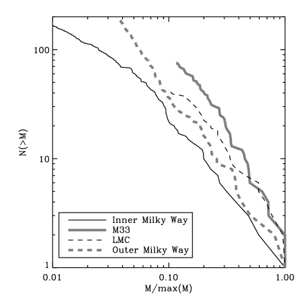
Figure 7: The cumulative mass distribution in three Local Group galaxies, with the inner and outer Milky Way plotted separately. This plot shows that there are significant differences in the mass spectrum from galaxy to galaxy, with the inner Milky Way giving a power law in dN/dM of -1.6, and M33 giving a power law index of -2.3.

We may also ask whether the clouds show differences, for example, in the size-linewidth relation observed for clouds in the Milky Way. Figure 8 shows a plot of hundreds of clouds in the Milky Way, M33, and the LMC, with a line of slope 1/2 superimposed on the data. Evidently, the clouds in these galaxies obey the same size-linewidth relation with no zero-point offset: $\Delta V\propto R^{1/2}$.

r

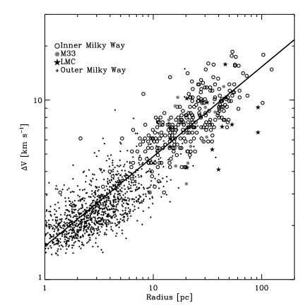
Figure 8: Size-linewidth relation for resolved GMCs in the same galaxies plotted in Figure 7. The clouds in all three galaxies appear to follow the same relation with $\Delta V\propto R^{1/2}$. Corrections have been applied to the published data to treat all of the data identically, and to correct for beam effects.

This plot suggests that if all of the clouds in these galaxies are self-gravitating, the surface density of the clouds is constant with a relative scatter given by the scatter in Figure 8. That is, since $\Delta V\propto R^{1/2}$, and $M\propto R(\Delta V)^{2}$/G, then $M/R^{2}=const$. But the mean internal pressure of GMCs can be written: $P_{int}$ = $\alpha(\pi/2)G{\Sigma_{g}}^{2}$, where $\Sigma_{g}$ is the gas surface density of the clouds and $\alpha$ is a constant near unity that depends on the cloud geometry. Thus, the GMCs that compose Figure 8 have the same mean internal pressure, regardless of size, regardless of the galaxy they are in and regarless of the external pressure.

This gives us a way of understanding how the IMF might indeed be constant from galaxy to galaxy, at least for galaxies similar to those in Figure 8. That is, if the mean internal pressure of all GMCs in the disk of a galaxy is the same, then the range of pressures within a GMC might also be the same, and the star-forming cores might therefore also be quite similar. It is important to keep in mind, however, that even if true it might apply only in the disks of galaxies. In the bulge regions, the hydrostatic pressure of the gas is likely to be two to three orders of magnitude higher than that in the disk (e.g. Spergel & Blitz (1992) $\!{}^{{\bf?}}$. In these regions, the external pressure can significantly exceed the mean internal pressure of a few $\times 10^{5}$ cm^-3 K of the clouds in the disk. In the bulge regions, the GMCs must be different from those in the disk, and may well give rise to stars with a different IMF.

Studying global star formation is only in its infancy and new instruments coming on line and being developed should provide the sensitive high resolution data needed to get from single star formation to the Madau plot. Equally important is to have those who work on local star formation interact closely with those working on global star formation on a regular basis as has happened in this conference.

References

References

- [1] Abel, T., Bryan, G. L., & Norman, M. L. 2002, Science, 295, 93
- [2] Alves, J. F., Lada, C. J., & Lada, E. A. 2001, Nature, 409, 159
- [3] Blitz, L., & Rosolowsky, E. 2004, ApJL, 612, L29
- [4] Bonnell, I. A., Bate, M. R., & Zinnecker, H. 1998, MNRAS, 298, 93
- [5] Deul, E. R., & van der Hulst, J. M. 1987, A&AS, 67, 509
- [6] Engargiola, G., Plambeck, R. L., Rosolowsky, E., & Blitz, L. 2003, ApJS, 149, 343
- [7] Lada, E. A. 1992, ApJL, 393, L25
- [8] Madau, P., Ferguson, H. C., Dickinson, M. E., Giavalisco, M., Steidel, C. C., & Fruchter, A. 1996, MNRAS, 283, 1388
- [9] Motte, F., Andre, P., & Neri, R. 1998, A&AS, 336, 150
- [10] Mizuno, N., et al. 2001, PASJ, 53, 971
- [11] Phelps, R. L., & Lada, E. A. 1997, ApJ, 477, 176
- [12] Rosolowsky, E., Engargiola, G., Plambeck, R., & Blitz, L. 2003, ApJ, 599, 258
- [13] Rosolowsky, E., & Blitz, L. 2005, ApJ, in press
- [14] Rowan-Robinson, M. 2001, ApJ, 549, 745
- [15] Shu, F. H. 1977, ApJ, 214, 488
- [16] Shu, F. H., Adams, F. C., & Lizano, S. 1987, ARA&A, 25, 23
- [17] Shu, F. H., Li, Z., & Allen, A. 2004, ApJ, 601, 930
- [18] Spergel, D. N., & Blitz, L. 1992, Nature, 357, 665
- [19] Stahler, S. W., Palla, F., & Ho, P. T. P. 2000, Protostars and Planets IV, 327
- [20] Steidel, C. C., Adelberger, K. L., Giavalisco, M., Dickinson, M., & Pettini, M. 1999, ApJ, 519, 1
- [21] Testi, L., & Sargent, A. I. 1998, ApJL, 508, L91
- [22] Williams, J. P., Blitz, L., & Stark, A. A. 1995, ApJ, 451, 252
- [23] Wong, T., & Blitz, L. 2002, ApJ, 569, 157