Correlated Mixture Between Adiabatic and Isocurvature
Fluctuations and Recent CMB Observations

Abstract

This work presents a reduced $\chi^{2}_{\nu}$ test to search for non-gaussian signals in the CMBR TT power spectrum of recent CMBR data, WMAP, ACBAR and CBI data sets, assuming a mixed density field including adiabatic and isocurvature fluctuations. We assume a skew positive mixed model with adiabatic inflation perturbations plus additional isocurvature perturbations possibly produced by topological defects. The joint probability distribution used in this context is a weighted combination of Gaussian and non-Gaussian random fields. Results from simulations of CMBR temperature for the mixed field show a distinct signature in CMB power spectrum for very small deviations ($\sim$ 0.1%) from a pure Gaussian field, and can be used as a direct test for the nature of primordial fluctuations. A reduced $\chi^{2}_{\nu}$ test applied on the most recent CMBR observations reveals that an isocurvature fluctuations field is not ruled out and indeed permits a very good description for a flat geometry $\Lambda$-CDM universe, $\chi^{2}_{930}$$\sim$ 1.5, rather than the simple inflationary standard model with $\chi^{2}_{930}$$\sim$ 2.3. This result may looks is particular discrepant with the reduced $\chi^{2}$ of 1.07 obtained with the same model in Spergel et al. (2003) for temperature only, however, our work is restricted to a region of the parameter space that does not include the best fit model for TT only of Spergel et al. (2003).

I Introduction

The new generation of cosmic microwave background radiation (CMBR) experiments has opened a new era in astrophysics, the precision cosmology era. Recent observations, especially those of WMAP (Wilkinson Anisotropy Microwave Probe), ACBAR (Arcminute Cosmology Bolometer Array Receiver) and CBI (Cosmic Background Imager), brought a new light to CMBR fluctuations studies in large, intermediate and small scales. This new generation of experiments made possible the characterization of the power spectrum of temperature fluctuations up to the third acoustic peak (Hinshwaw et al. 2003; Pearson et al. 2002; Kuo et al. 2004). Indeed, the combination of CMBR and large scale structure (LSS) data allows cosmologists to constrain cosmological parameters for a given set of scenarios and also determine the nature of the primordial fluctuations. Since CMBR carries the intrinsic statistical properties of cosmological perturbations, it is considered the most powerful tool to investigate the nature of cosmic structure.

The most accepted model for structure formation assumes initial quantum fluctuations created during inflation and amplified by gravitational effects. The standard inflation model predicts an adiabatic uncorrelated random field with a nearly flat, scale-invariant spectrum on scales larger than $\sim$ 1-2^∘ (Guth 1981; Salopek, Bond & Bardeen 1981; Bardeen, Steinhardt & Turner 1983). Simple inflationary models also predict the random field follows a nearly-Gaussian distribution, where only small deviations from Gaussianity are allowed (e.g. Gangui et al. 1994). In hybrid inflation models (Battye & Weller 1998; Battye, Magueijo & Weller 1999), structure is formed by a linear combination of (inflation-produced) adiabatic and (topological defects induced) isocurvature density fluctuations. The topological defects are assumed to appear during the phase transition that marks the end of the inflationary epoch.

Correlated mixed field with adiabatic and isocurvature fluctuations has been considered by many authors, as Bucher et al. (2000), Gordon (2001) and Amendola et al (2002). Andrade et al. (2004) have suggested a new mixed scenario describing a correlated mixture of two fields, one of them being a dominant Gaussian adiabatic process to which is added a small contribution of an isocurvature field. In a previous work, Ribeiro, Wuensche & Letelier (2000) used such mixed scenario to probe the galaxy cluster abundance evolution in the universe and found that even a very small level of non-Gaussianity in the mixed field may introduce significant changes in the cluster abundance rate. Andrade, Wuensche and Ribeiro (2004) showed the effects of mixed models in the CMBR power spectrum, combining a Gaussian (adiabatic) field with a second isocurvature field to produce a positive skewness mixed density fluctuation field. This approach adopted a scale dependent mixture parameter and a power-law initial spectrum to simulate the CMBR temperature and polarization power spectra for a flat $\Lambda$-CDM model, generating quite a large grid of cosmological parameters combination. The results show how the shape and amplitude of the fluctuations in CMBR depend upon such mixed fields and how we can easily distinguish a standard adiabatic Gaussian field from a mixed non-Gaussian one and easily quantify the contribution of the second component.

In this work, we apply a statistical test to both the mixed power spectrum simulations and recent CMBR data obtained by WMAP (Spergel et al. 2003), ACBAR (Kuo et al. 2004) and CBI (Pearson et al. 2002) in order to compare how well the standard and mixed models describe the most recent observations. We also estimate the possible contribution of an isocurvature field to the primordial density fluctuation field in the mixed model scenario.

II Recent CMB Observations

The experiments ACBAR and CBI present the highest sensitivity and highest signal to noise observations of CMBR temperature distribution in small angular scales ( $\sim$ 4 -5 arcminutes). In scales larger than the above mentioned ($\sim$ 20 arcminutes ) the WMAP satellite made a set of all-sky maps measuring both the temperature and polarization anisotropies, opening a new window for cosmological investigations.

The WMAP observations, combined with LSS observations has made possible to constrain a precise picture of the cosmos. Using the three-dimensional power spectrum P(k) from over 200,000 galaxies in the Sloan Digital Sky Survey (SDSS) in combination with WMAP and other data, Tegmark et al. (2003) show that recent observations are consistent with a flat adiabatic $\Lambda$-CDM model. Specifically, the CMB power spectrum exhibits a first acoustic peak at l = 220.1 $\pm$ 0.8, with amplitude of the 74.7 $\pm$ 0.5 $\mu$K ; and a second acoustic peak at l = 546 $\pm$ 10, with amplitude of 48.8 $\pm$ 0.9 $\mu$K, a picture consistent with inflation predictions (Peiris et al. 2003). The best fit model compared with the WMAP plus ACBAR and CBI is for a $\Lambda$-CDM Universe with the following cosmological parameter combination: $\Omega$_toth² = 1.02 $\pm$ 0.002; $h=0.71^{+0.04}_{-0.03}$; $\Omega_{CDM}h^{2}=0.0224\pm 0.0009$; $\Omega_{m}h^{2}=0.135^{+0.008}_{-0.009}$; $n_{s}(0.05Mpc^{-1})=0.93\pm 0.03$ and a slope running spectral index with $dn_{s}/dln(k)=-0.031^{+0.016}_{-0.018}$ (Spergel et al. 2003). The present CMBR data provides a strong support for adiabatic field domination.

However, the WMAP data show several peculiarities at various values of l. WMAP observations show that the fluctuations in large scale present a lower amplitude than the standard inflation model predicts. The temperature power spectrum is almost 30% suppressed on $\sim$ 1 degree angular scales (Hinshaw et al., 2003), specially those scales related to the quadrupole (l = 2) and the octopole (l = 3), when compared with the predictions of the standard gaussian $\Lambda$-CDM models. Another impressive WMAP conclusions is the evidence of an optical depth to re-scattering by electrons with a value of $\tau$ = 0.17 $\pm$ 0.04, describing a reionization scenario at redshift 11 $\leq$ z $\leq$ 30 (Kogut et al. 2003).

In this paper, we try to reproduce the main feature of the CMBR power spectrum, in large, intermediate and small scales, invoking just the primordial physics, by considering a correlated mixed field in combination with six cosmological parameters: $\Omega$_b, $\Omega$_cdm, $\Omega$_Λ, n, H₀, the amplitude of the power spectrum, A, and the mixed coefficient, $\alpha$₀. Since we are interested in just cosmological principles, no secondary effects are considered in CMB fluctuations, like reionization models, gravitational lenses nor Sunyayev-Zeldovich effects.

III The Mixed Model

III.1 The Mixed Primordial Power Spectrum

In the mixed scenario, we suppose that the field has a probability density function of the form:

$${\cal P}[\delta_{k}]~{}\propto~{}(1-\alpha)f_{1}(\delta_{k})+\alpha f_{2}(\delta_{k})$$ (1)

The first field will always be the Gaussian component and a possible effect of the second component is to modify the Gaussian field to have a positive tail. The parameter $\alpha$ in (1) allows us to modulate the contribution of each component to the resultant field. Like the hybrid inflation models (Battye & Weller 1998; Battye, Magueijo & Weller 1999), the mixture models consider the scenario in which structure is formed by both adiabatic density fluctuations produced during inflation and active isocurvature perturbations created by cosmic defects during a phase transition which marks the end of inflationary epoch.

Nevertheless, the mixed scenario considers a possible correlation between the adiabatic and the isocurvature fields on the post-inflation Universe. So, the fluctuations in super-horizon scales (inflated during the exponential expansion) are strictly uncorrelated and the mixing effect acts only inside the Hubble horizon, in sub-degree scales. To allow for this condition and keep a continuous mixed field, a scale dependent mixture parameter, $\alpha$ $\equiv$ $\alpha$(k) was defined. We assume the simplest choice of $\alpha$(k), a linear function of $k$:

$$\alpha(k)\equiv\alpha_{0}k$$ (2)

To constrain the two component random field, we take $\delta_{k}=P(k)\nu^{2}$, where $\nu$ is a random number with distribution given by (1). So, we consider the primordial power spectrum of the mixed field in the form:

$$P(k)^{mix}\equiv M^{mix}(\alpha_{0},k)P(k)$$ (3)

where the $P(k)$ represents a primordial conventional power-law spectrum and M^mix($\alpha$) is the mixture term, a functional of $f_{\mathit{1}}$ and $f_{\mathit{2}}$, which account for the statistics effect of a new component:

$$M^{mix}(\alpha_{0},k)\equiv\int_{\nu}[(1-\alpha_{0}k)f_{1}(\nu)+\alpha_{0}kf_{2}(\nu)]\nu^{2}\;d\nu$$ (4)

The effective mixed primordial power spectrum is expressed as:

$$P(k)^{mix}=k^{n}+M(\alpha_{0})k^{n+1}$$ (5)

where M($\alpha$₀) represents only the coefficient dependence, $\alpha$₀. In the case of a pure Gaussian field, M($\alpha$₀) $\approx$ $\alpha$₀ $\approx$ 0, the mixed power spectrum will be a simple power-law spectrum, $k^{n}$, where n is the conventional spectral index predicted by inflationary models. In the case of a mixed field, the phase correlations between both fields are estimated by the integral in Eq.(4), on mixture scales defined by Eq. (2).

III.2 The Evolution of The Mixed Field

To estimate the CMBR anisotropy we need to evaluate the evolution of fluctuations field generated in the early universe through the radiation-dominated era and recombination. In the mixed model, the evolution of both adiabatic and isocurvature components of the mixed density field is considered an independent process, when only their effective amplitude correlation is considered on the decoupled surface of the CMBR photons.

To compute the independent evolution of the adiabatic $\Lambda$-CDM mode and the isocurvature $\Lambda$-CDM mode, we have used the most precision code, the Linger function of the COSMICS code package (Bertschinger 1999; Ma & Bertschinger 1995). Linger does generate the most accurate results for the photon density field, being able to compute the CMBR anisotropy with integrations errors less than 0.15%. However, Linger routine is very time consuming, but for investigation of small deviations from gaussianity, the COSMICS package seems to be the most precise code for mixed CMB simulations.

Once estimated the photon density evolution, the multipole moments, C_l, of the CMBR temperature power spectra were estimated by a mixed photon density function incorporated to the original COSMICS package:

$$C_{l}=4\pi\int_{0}^{k_{max}}\;d^{3}kP^{mix}(k)(\Delta_{l}^{mix})^{2}(k,\tau)$$ (6)

The function $\Delta_{l}^{mix}$ represents the mixed photon density field in the last scattering surface defined by:

$$\Delta_{l}^{mix}\equiv(1-\alpha_{0}k)\Delta_{l}^{Adi}+\alpha_{0}k\Delta_{l}^{Iso}$$ (7)

where $\Delta_{l}^{Adi}$ and $\Delta_{l}^{Iso}$ are the photon density function estimated by COSMICS, respectively, for an adiabatic and an isocurvature seed initial conditions.

Inserting (7) in (6), we obtain a mixed term in the C_l estimation. This condition suggests that the amplitude of both fields are cross-correlated at the last scattering surface, with a mixing ratio defined by $\alpha$₀ and in a characteristic scale defined by $\alpha$₀k. The power spectra estimated by Eq.(3) consider a flat $\Lambda$-CDM universe slightly distorted by a non-gaussian statistics with constant spectral index.

A number of realizations of CMBR temperature power spectra were made and the mean temperature fluctuations combining Gaussian, Exponential, Lognormal, Rayleigh, Maxwellian and a Chi-squared distributions was estimated (Andrade et al. 2004). The simulations show that the influence of the specific statistics of the second component in the mixed field is not so important as the cross-correlation between the amplitudes of both fields. However, some important results were obtained. It is possible to directly assess and quantify the mixture of a correlated adiabatic and isocurvature non-Gaussian field. This behavior points to another possibility to extract information from a CMBR power spectrum: the possibility of detecting weakly mixed density fields, even if we can not exactly identify the mixture components distribution.

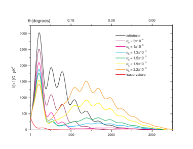
Figure 1: CMBR temperature mixed angular power spectrum estimated for a $\Lambda$-CDM model in different mixing degrees.

In Figure 1, we see how the shape and amplitude of the spectrum change even for small values of $\alpha$_o ($\sim$10^-4-10^-3). The peaks intensities are clearly susceptible to the existence of mixed fields, although distinguishing peaks of higher order (2^nd, 3^rd, etc.) in the mixed context is not a straightforward task, since their intensities, compared to the first peak, are very low. The effect of increasing $\alpha$₀ is a power transfer to smaller scales (l >1000), while the super-degree scales are less affected. However, for large values of $\alpha$₀ ($\alpha$₀ >3x10^-3) there is a fast increase in the temperature fluctuations, probably caused by correlation excess between the mixed fields, resulting in more power in small scales. Therefore, an acceptable range for $\alpha_{0}$ is set to be $\alpha_{0}\lesssim 3\times 10^{-3}$.

IV A $\chi^{2}$ Test on CMB Observation

In order to quantify a possible non-gaussian isocurvature contribution to the fluctuations field, we applied a maximum likelihood approach to the power spectrum estimated by the most recent CMBR observations. We ran a set of CMBR realizations for mixed and pure density fields, considering a flat $\Lambda$-CDM Universe consistent with inflation predictions and LSS observations.

Instead of the usual CMBR analysis approach, which considers tensors contribution and reionization effects, we consider only the main six cosmological parameters ($\omega_{cdm}$, $\omega_{b}$, $\omega$_Λ, n, H₀, $\alpha_{0}$), and also A, described in the range of possibilities: 0.8< n <1.2; 0.015 <$\Omega$_b< 0.03; 0.6 <$\Omega$_Λ< 0.8; 60 <H₀< 80; cold dark matter density set as 1-($\Omega$_b + $\Omega$_Λ), ranging of 0.170 < $\Omega$_cdm< 0.385; and the range values of $\alpha$₀ set in 0.0 < $\alpha$₀ < 3x10^-3. With this considerations, we ensure the simulations are in agreement with the basic preferences of standard inflation scenarios: flat geometry ($\Omega$_tot $\sim$ 1) and a nearly scale invariant primeval spectrum (n $\sim$ 1). $\Omega$_b =(0.019 $\pm$ 0.01)h^-2 is consistent with the mass density of baryons determined by Big Bang nucleossynthesis and the large scale structure observations, which suggests that the Hubble constant H₀ assumes values in the range (66 < H₀ < 75) km/sec.Mpc; and a positive cosmological constant value in the range (0.065< $\Omega$_Λ <0.75), as estimated recently by Tegmark et al. (2003). The amplitude of the primordial power spectrum, A, was estimated by the best fit value for each model simulated.

We applied a reduced $\chi^{2}$ test (Bevington 1969) between the CMB data and the power spectra simulations in the mixed context in four steps. First, we consider the WMAP, CBI and ACBAR data independently, estimate the reduced $\chi^{2}$ for all three data sets and then add all data to obtain a new estimation of the reduced $\chi^{2}$. So we estimate the residual difference for C_l estimation in $\mu$K², and consider the power spectrum data points (899 for WMAP; 24 for CBI and 14 for ACBAR) minus 7 degree of freedom. We create a grid of nearly one hundred simulated values of $\alpha$₀ for each combination of standard cosmological parameters. Since COSMICS is very time consuming, the variations in the standard cosmological parameters were set in order to give just the main direction for the $\chi^{2}$ face variations in cosmological parameters. The most precise models, as defined by the $\chi^{2}$ test, are summarized on Table 1, which also contains the best $\alpha$₀ value estimated for each parameter combination listed with 68% confidence limit.

$H_{0}$	$\Omega_{b}$	$\Omega_{\Lambda}$	n	2$\pi$A	$\alpha_{0}$	WMAP	CBI	ACBAR	All data	$Best\alpha_{0}$
(km$s^{-1}Mpc^{-1}$)				($\mu$$K^{2}$)		$\chi^{2}_{892}$	$\chi^{2}_{24}$	$\chi^{2}_{7}$	$\chi^{2}_{930}$	$\Delta\alpha_{0}$
70	0.015	0.8	1.1	92.462	0.0	2.820	1.121	2.925	2.754	0.00066
70	0.015	0.8	1.1	117.558	5x$10^{-4}$	1.590	2.999	7.259	1.677	$\pm$ 0.00045
70	0.015	0.7	1.1	113.326	0.0	3.532	1.480	3.372	3.451	0.00061
70	0.015	0.7	1.1	152.947	5x$10^{-4}$	1.779	3.608	9.236	1.888	$\pm$ 0.00036
70	0.015	0.6	1.1	130.444	0.0	4.324	1.934	5.485	4.234	0.00056
70	0.015	0.6	1.1	183.351	5x$10^{-4}$	2.703	4.288	11.314	2.387	$\pm$ 0.00033
70	0.023	0.8	1.1	87.918	0.0	2.422	1.000	2.796	2.379	0.00057
70	0.023	0.8	1.1	110.492	5x$10^{-4}$	1.474	2.543	5.269	1.543	$\pm$ 0.00048
70	0.023	0.7	1.1	109.225	0.0	2.899	1.117	2.982	2.857	0.00052
70	0.023	0.7	1.1	145.041	5x$10^{-4}$	1.560	2.875	6.959	1.651	$\pm$ 0.00034
70	0.023	0.6	1.1	126.660	0.0	3.573	1.528	4.632	3.539	0.00047
70	0.023	0.6	1.1	175.405	5x$10^{-4}$	2.031	3.602	9.144	2.132	$\pm$ 0.00030
70	0.030	0.8	1.1	84.160	0.0	2.124	1.000	3.336	2.103	0.00047
70	0.030	0.8	1.1	104.347	5x$10^{-4}$	1.490	2.270	4.663	1.555	$\pm$ 0.00036
70	0.030	0.7	1.1	106.037	0.0	2.274	1.009	3.001	2.269	0.00042
70	0.030	0.7	1.1	137.782	5x$10^{-4}$	1.433	2.538	5.938	1.522	$\pm$ 0.00030
70	0.030	0.6	1.1	123.570	0.0	2.756	1.404	4.299	2.776	0.00038
70	0.030	0.6	1.1	166.921	5x$10^{-4}$	1.855	3.146	7.950	1.956	$\pm$ 0.00029
60	0.030	0.7	1.1	92.088	0.0	2.697	1.001	3.371	2.657	0.00063
60	0.030	0.7	1.1	118.071	5x$10^{-4}$	1.590	2.463	5.355	1.646	$\pm$ 0.00046
65	0.030	0.7	1.1	99.315	0.0	2.410	1.001	2.791	2.383	0.00052
65	0.030	0.7	1.1	128.530	5x$10^{-4}$	1.382	2.344	5.398	1.456	$\pm$ 0.00036
75	0.030	0.7	1.1	112.147	0.0	2.212	1.243	3.707	2.231	0.00033
75	0.030	0.7	1.1	145.624	5x$10^{-4}$	1.680	2.847	6.784	1.780	$\pm$ 0.00030
80	0.030	0.7	1.1	117.683	0.0	2.192	1.492	4.894	2.242	0.00026
80	0.030	0.7	1.1	151.419	5x$10^{-4}$	2.081	3.228	8.150	2.190	$\pm$ 0.00030
70	0.030	0.7	1.0	73.291	0.0	1.887	1.002	2.463	1.863	0.00027
70	0.030	0.7	1.0	92.857	5x$10^{-4}$	1.668	2.855	6.798	1.778	$\pm$ 0.00034
70	0.030	0.7	1.2	151.783	0.0	2.886	1.008	3.750	2.917	0.00056
70	0.030	0.7	1.2	202.597	5x$10^{-4}$	1.425	2.261	5.267	1.490	$\pm$ 0.00037

Table 1: The reduced $\chi^{2}$ test applied on the WMAP, CBI and ACBAR data and the power spectrum simulations in a mixed scenario for some $\Lambda$-CDM models. The last column shows the best $\alpha$₀ estimation for each model with 68% confidence limit

The simulations clearly show that WMAP data tends to favor mixed models. The $\chi^{2}_{\nu}$ estimated for the fit between mixed models and WMAP data are significatively lower for mixing degrees of order $\sim$$10^{-3}$, in all combination of cosmological parameters tested. However, CBI and ACBAR data in small angular scales tends to favor the adiabatic standard models. The combination of all data are more sensible to WMAP influence (more signal in large and intermediate scales with low error bars) resulting in best fits models in a mixed scenario. All data favor a $\Lambda$-CDM Universe with contents of barions, dark matter and dark energy coherent with that estimated by the WMAP and LSS analysis.

Figure 2 shows the powers spectrum of the standard adiabatic and mixed models for the three best fit models obtained by the $\chi^{2}_{\nu}$ test. It also shows the behavour of the all data $\chi^{2}_{\nu}$ while varying the $\alpha$₀ value. It is clearly seen that the mixed model adjust the data better than the standard model in basic combination of cosmological parameters. In this figure, is possible to observe that the relation between the amplitudes of the acoustic peaks in the mixed scenario is more adequate to describe the CMBR power spectrum feature without consideration of any model of reionization or tensors contributions. Although the mixed model predicts higher quadrupole and octopole contributions that predicts the standard adiabatic $\Lambda$-CDM model, the plots clearly show that the mixed predictions are consistente with acoustic peaks amplitude estimated by WMAP. Indeed, a model estimation in a good fit is obtained for a strictly flat Universe, rather than an open Universe or, instead, a slope running spectral index (Kosowsky & Turner, 1995) as suggested by the WMAP team.

One possible explanation of the low amplitude in large scales and the high amplitude of the secondary acoustic peaks predicted by the standard model (pure adiabatic) simulated in this work is the lack of the high optical depth, as considered by the WMAP team (Hinshaw et al. 2003; Spergel et al. 2003). Reionization affects the CMBR in several manners, through Thomson scattering of photons from free electrons in the intergalactic medium, which suppress the primordial anisotropies of the CMBR imprinted on the decoupled surface. In a reionizing scenario, the acoustic peaks in the CMBR power spectrum would have the amplitude lowered by $e^{-2\tau}$ and the rescattering would generate large angle temperature fluctuations through the Doppler effect (Hu & White, 1997). In this work, rather than considering reionization effects and invoking just primordial physics, we can explain the main feature of the CMBR power spectrum in large, intermediate and small scales in the context of mixed density field.

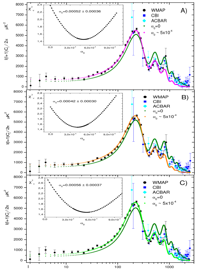
Figure 2: CMBR temperature power spectrum estimated for the best three parameter combination: $\Omega$_b= 0.03; $\Omega$_CDM= 0.27; $\Omega$_Λ= 0.7. In A: H₀= 65Km/sMpc and n=1.1; in B: H₀= 70Km/sMpc and n=1.2; in C: H₀= 70Km/sMpc and n=1.1. The small picture in figures show the behavior of $\chi^{2}_{\nu}$ while varying $\alpha$₀ value

V Discussion

We applied a modified statistical $\chi^{2}_{\nu}$ test to the most recent CMBR observations. The results allow us to compare the performance of power spectra simulated with mixed and standard density fields to describe the mean feature of CMBR temperature fluctuations. The results showed that the WMAP data tends to favor mixed density fields with isocurvature fluctuation contribution of order $\sim$$10^{-3}$ ($\chi^{2}_{892}$$\sim$ 1.5 for mixed model against $\chi^{2}_{892}$$\sim$ 2.4 in standard models) without the need of considering any model of reionization. Also, large scale fluctuations are in good agreement with WMAP measurements. Our result may looks discrepant with the reduced $\chi^{2}$ of 1.07 obtained with the same model in Spergel et al. (2003) for temperature only, however, our work is restricted to a region of the parameter space that does not include the best fit model for TT only of the WMAP team. We can conclude that the mixed scenario offers a good alternative to describe the shape of TT CMBR power spectrum. Indeed, the data favors a $\Lambda$-CDM Universe with barions, dark matter and dark energy contents which are coherent with a strictly flat Universe, with no need to include tensor contributions nor a slope running spectral index. For a $\Lambda$-CDM Universe with contents of $\Omega$_b= 0.03; and the best value indicated for the spectral index, by the $\chi^{2}$ test, n$\sim$1.1; the contribution of the isocurvature field is estimated as $\alpha$₀= 0.00042 $\pm$ 0.0003 with 68% confidence limit.

Although the standard $\Lambda$-CDM model fits well a small number of data points of CBI ($\chi^{2}_{24}$$\sim$ 1 for standard models against $\chi^{2}_{24}$$\sim$ 2.3 in mixed models) and ACBAR ($\chi^{2}_{7}$$\sim$ 2.4 for standard models against $\chi^{2}_{7}$$\sim$ 6.8 in mixed models), when considering all data points, CBI, ACBAR and WMAP, the mixed model clearly shows ability to describe the mean feature of TT CMBR observation in large, intermediate and small scales. With the upcoming generation of experiments which will probe temperature fluctuations in small scales, such as Planck satellite, it will be possible to set new, more stringent, estimates of the parameter spaces and isocurvature fluctuations contributions. Also, we will try to constrain the mixed model predictions upon the temperature-polarization cross correlated power spectrum, in order to consider reinonizations models in the mixed scenario. Presently, we conclude that isocurvature fluctuations can not be ruled out in cosmological studies. Also, conflicting with the results of WMAP map team (Komatsu et al. 2003), the results of some independent searches for non-gaussianity in WMAP maps evidence that WMAP data are consistent with gaussian condition for l <250, marginally gaussian for 224<l <350, and non-gaussian for l >350, as revealed, for instance, by the phase mapping technique (Chiang et al. 2003; Coles et al. 2003). This picture points an extra expectation in the study of the mixed model predictions, altough, in order to constrain a better estimative of $\alpha$₀, reionizations models must be investigated in the context of mixed fields.

The next step in the investigation of the mixed models in CMBR features will be the predictions of the reionization effects, even in a low redshifts, the degeneraices between cosmological parameters in mixed context, the predictions of the angular correlation function and the temperature-polarization cross correlated power spectrum.

- (1) Amendola L. et al., 2002, Phys. Rev. Lett., 88, 211302.
- (2) Andrade A.P.A., Wuesnche C.A., Ribeiro A.L.B., 2004, ApJ, 602, 555.
- (3) Bardeen J.M., Steinhardt P.J., Turner M.S., 1983, Phys. Rev.D, 28, 679.
- (4) Battye R.A., Weller J., 1998, in Montmerle P. J., Auborg E., eds., The 19th Texas Symposium on Relativistic Astrophysics and Cosmology, Paris, France.
- (5) Battye R.A., Magueijo J., Weller J., 1999, astro-ph/9906093.
- (6) Bertschinger E., 1999, COSMICS: Cosmological Initial Conditions and Microwave Anisotropy Codes, Massachusetts Institute of Technology, (http://arcturus.mit.edu/cosmics).
- (7) Bevington P. R. , Data Reduction and Error Analysis for the Physical Sciences. New York: McGraw-Hill, 1969.
- (8) Bucher M. et al., 2000, Phys. Rev. D, 62, 083508.
- (9) Chiang, LY., Naselsky, P.D., Verkhodanov, O.L., Way, M.J., 2003, ApJ, 590, L65.
- (10) Coles P. et al., 2003, MNRAS, astro-ph/0310252.
- (11) Djorgovski S.G et al., 2001, ApJ, 560, L5.
- (12) Fan X. et al., 2001, Astron.J., 122, 2833.
- (13) Gangui A. et al., 1994, ApJ, 430, 447.
- (14) Gordon, C. et al., 2001, Phys. Rev. D, 63, 23506.
- (15) Guth A.H., 1981, Phys. Rev. D, 23, 347.
- (16) Haiman Z., Holder G.P., 2003, ApJ, 595, 1.
- (17) Hinshaw G. et al., 2003, ApJ, 148, 135.
- (18) Hu W., White M., 1997, New Astron., 2, 323.
- (19) Kogut, A. et al., 2003, ApJ, 148, 161.
- (20) Komatsu E. et al., 2003, ApJ, 148, 119.
- (21) Kosowsky A., Turner M., 1995, Phys. Rev. D, 52, 1739.
- (22) Kuo C.L. et al, 2004, ApJ, 600, 32.
- (23) Ma C., Bertschinger E., 1995, ApJ, 455, 721.
- (24) Pearson, T.J. et al., 2002, ApJ, 591, 556.
- (25) Peiris, H.V. et al., 2003, ApJ, 148, 213.
- (26) Ribeiro A.L.B., Wuensche C.A., Letelier P.S., 2000, ApJ, 539, 1.
- (27) Salopek D., Bond J. R., Bardeen J. M., 1989, Phys. Rev. D, 40, 1753.
- (28) Spergel, D.N., et al., 2003, ApJ, 148, 175.
- (29) Tegmark M. et al., 2003, astro-ph/0310723.
- (30) Turner M.S., 1998, in Caldwell D., Ed, The Proceedings of Particle Physics and the Universe (Cosmo-98), Woodbury, NY.