A new method optimized to use Gamma Ray Bursts as cosmic rulers

Abstract

We present a new method aimed to handle long Gamma–Ray Burst (GRBs) as cosmic rulers. The recent discovery of a tight correlation between the collimation corrected GRB energy and the peak of the $\gamma$–ray spectrum has opened the possibility to use GRBs as a new category of standard candles. Unfortunately, because of the lack of low–$z$ GRBs, up to now this correlation is obtained from high–$z$ GRBs with the consequence that it depends on the cosmological parameters we pretend to constrain. Hopefully this circularity problem will be solved when, in a few years, the low–$z$ GRB sample will be increased enough. In the meanwhile we present here a new Bayesian method that eases the aforesaid circularity problem, and allows to introduce new constrains on the cosmological $(\mbox{$\Omega_{\rm M}$},\mbox{$\Omega_{\Lambda}$})$ diagram as well as to explore the universe kinematics up to $z\approx 3$. The method we propose offers the further advantage to make handy the problem of the $(\mbox{$\Omega_{\rm M}$},\mbox{$\Omega_{\Lambda}$})$ loitering line singularity which inevitably appears when standard candles with $z>2$ are used. The combination of GRB with SN Ia data makes the popular $\Lambda$CDM cosmology more consistent with the Hubble diagram at a 68% confidence level. For a flat cosmology we find $\mbox{$\Omega_{\rm M}$}=0.28\pm 0.03$ for the combined GRB+SN Ia data set. Correspondingly, the transition redshift between cosmic deceleration and acceleration is $z_{\rm T}=0.73\pm 0.09$, slightly larger than the value found by considering SNe Ia alone. We briefly discuss our results also in terms of non–$\Lambda$CDM dark energy models.

1 Introduction

Figure 1: Rest frame correlations between the spectral peak energy $E_{\rm peak}$ and the collimation corrected energy $E_{\gamma}$ (left panel), the collimation angle $\theta$ (middle) and the isotropic bolometric energy (right), for the 15 GRBs considered in GGL, assuming $\Omega_{\rm M}$=0.3 and $\Omega_{\Lambda}$=0.7. Different symbols (colors) correspond to different redshift ranges: circles (blue), triangles (green) and squares (red) are for $z<0.7$, $0.7<z<1.55$ and $z>1.55$, respectively. The solid line in the left panel represents the best fit $E_{\rm peak}$–$E_{\gamma}$ correlation ($\chi^{2}=1.27$) and the shaded region its uncertainty computed in the coordinate frame where the variances on its parameters are uncorrelated. We also show (open circle) the recent GRB 041006 (data in Galassi et al. 2004, D’Avanzo et al. 2004 and the HETE2 web page (http://space.mit.edu/HETE/Bursts/GRB041006).

The Hubble diagram of type Ia Supernovae (SNe Ia) has revolutionized cosmology, showing that the current expansion of the universe is accelerated (Riess et al. 1998; Riess et al. 2004; Perlmutter et al. 1999), with a possible transition from deceleration to acceleration at low redshifts (Riess et al. 2004; Dicus & Repko 2004). The most popular explanation for the recent acceleration implies the existence of a dominant energy density component with negative pressure (dark energy, see for a recent review Sahni 2004). Its physical nature is still a mystery. The simplest candidate for dark energy is the modern version of the Einstein cosmological constant $\Lambda$, which, however, raises several theoretical difficulties (see Padmanabhan 2003; Peebles & Ratra 2003; Sahni 2004). There is now a flurry of activity focused to unveil the nature of dark energy or to constrain any alternative explanation to accelerated expansion. The forthcoming SNAP mission ($z_{\rm max}\approx 1.7$) will offer an unprecedented accuracy on this undertaken. Besides accuracy, also a survey reaching larger redshifts is desirable in order to overcome parameter degeneracies, and to study the evolution of dark energy (Linder & Huterer 2003; Weller & Albrecht 2002; Nesseris & Perivolaropoulos 2004). Furthermore, alternative standard candles to SNe Ia, free of extinction issues, are also highly desired. Long GRBs have been pointed out as possible candidates to be these high–redshift candles (Schaefer 2003), and in Ghirlanda et al. (2004b, GGLF thereafter) we have shown that they are indeed.

Assuming isotropy, the energy emitted by GRBs in $\gamma$–rays ($E_{\rm iso}$) is spread over 4 orders of magnitude, but the presence of an achromatic break in their afterglow lightcurve is a strong evidence that their emission is collimated into a cone of semiaperture angle $\theta$ (e.g. Rhoads 1997; Sari, Piran & Halpern 1999). Correcting for this anisotropy, the resulting $\gamma$–ray energetics $E_{\gamma}=(1-\cos\theta)E_{\rm iso}$ clusters around $E_{\gamma}\sim 10^{51}$ erg, with a small dispersion (0.5 dex, Bloom, Frail & Kulkarni 2003; Frail et al. 2001), yet not small enough for a cosmological use (Bloom, Frail & Kulkarni 2003).

Recently, a very tight correlation has been found (Ghirlanda, Ghisellini & Lazzati 2004a, GGL thereafter) between $E_{\gamma}$ and the peak energy $E_{\rm peak}$ of the prompt emission (in a $\nu F_{\nu}$ representation) (§2). This correlation has been used for a reliable estimate of $E_{\rm iso}$, and therefore of the luminosity distance, with the aim to construct a Hubble diagram up to $z=3.2$ (GGLF; Dai, Liang & Xu 2004).

The existence of the $E_{\gamma}$–$E_{\rm peak}$ correlation, allowing to know the intrinsic emission of GRBs, makes them standard candles similar to SNe Ia and Cepheid stars. Hopefully, this correlation will be calibrated from low–$z$ GRBs, and corroborated by a robust theoretical interpretation. Currently low–$z$ GRBs are scarce: we must wait for a few years before having a sufficient number of GRBs at $z<$0.2. For the time being, the correlation is obtained from high–$z$ GRBs with the consequence that it depends on the cosmological parameters which we pretend to find. We present here a new method with respect to GGLF that eases this difficulty making possible the full use of the available information. We will assume that the $\Lambda$CDM cosmology has $h=0.71$, $\mbox{$\Omega_{\rm M}$}=0.27$, and $\mbox{$\Omega_{\Lambda}$}=0.73$.

2 The $E_{\gamma}$–$E_{\rm peak}$ correlation

In Fig. 1 (left panel) we show the correlation between the rest frame $E_{\rm peak}$ and $E_{\gamma}$ for the 15 bursts considered by GGL, using the data listed in their Tab. 1 and Tab. 2, and assuming $\Omega_{\rm M}=0.3$ and $\Omega_{\Lambda}=0.7$. With this choice of cosmology, the reduced $\chi^{2}=1.27$ for the fit with a powerlaw. The mid panel shows $E_{\rm peak}$ as a function of the jet aperture angle $\theta$, while the right panel shows $E_{\rm peak}$ as a function of the isotropic emitted energy $E_{\rm iso}$ (the “Amati” relation, Amati et al. 2002) for the same 15 bursts. Also shown is the recent GRB 041006: although fully consistent with the GGL correlation, it is not included in the sample of 15 GRBs used for cosmology due to the still unpublished uncertainties on the relevant parameters. The shaded area in the left panel shows the region of uncertainties of the best fit correlation: $E_{\rm peak}/(263\pm 15~{}{\rm keV})=[E_{\gamma}/(4.2\times 10^{50}{\rm erg})]^{0.706\pm 0.047}$. The errors on its slope and normalization are calculated in the “baricenter” of $E_{\rm peak}$ and $E_{\gamma}$, where the slope and normalization errors are uncorrelated (Press et al. 1999). For similar $E_{\rm peak}$, there is a distribution of jet aperture angles, which is why $E_{\gamma}$, for a given $E_{\rm peak}$, is much less spread than the corresponding $E_{\rm iso}$ values.

In the present sample of bursts with known redshift GRB 980425 (Galama et al. 1998) and GRB 031203 (Gotz et al. 2003) are outliers for both the $E_{\rm peak}-E_{\rm iso}$ and the $E_{\gamma}-E_{\rm peak}$ correlation. These events are indeed peculiar for their small prompt and afterglow emission, as recently discussed by Soderberg et al. (2004a). It has been also suggested that these two events are sub–energetic, with respect to ´´classical´´ GRBs, because they are observed off–axis (Waxman 2004; Yamazaki, Yonetoku & Nakamura 2003). Also GRB 020903 (Soderberg et al. 2004b) may be an outlier for the $E_{\gamma}-E_{\rm peak}$ correlation, although, as discussed in GGL, its afterglow data are not conclusive.

3 The method

A Friedmann-Robertson-Walker cosmological model is defined by the Hubble parameter $H(z)$ given by:

$$H^{2}(z)=H_{0}^{2}\left[\mbox{$\Omega_{\rm M}$}(1+z)^{3}+\mbox{$\Omega_{k}$}(1+z)^{2}+\mbox{$\Omega_{\rm E}$}f(z)\right]$$ (1)

where $\mbox{$\Omega_{k}$}=1-\mbox{$\Omega_{\rm M}$}-\mbox{$\Omega_{\rm E}$},$ $\Omega_{\rm M}$ and $\Omega_{\rm E}$ are the present–day density parameters of matter and dark energy components, and $f(z)$ is a function that depends on the equation-of-state index of the dark energy component, $w(z)=p_{\rm E}(z)/\rho_{\rm E}(z)c^{2}$. Later on we will take into account the case of a cosmological constant ($\Lambda$–models) with $\mbox{$\Omega_{\rm E}$}=\mbox{$\Omega_{\Lambda}$}$, $w=-1$ and $f(z)=1$, as well as a linear parametrization of the dark energy equation of state ($W_{i}$–models) adopting $w(z)=w_{0}+w^{\prime}z$, a flat cosmology, and $f(z)=(1+z)^{3(1+w_{0}-w^{\prime})}\exp(3w^{\prime}z)$. Once defined $H(z)$, the luminosity distance as a function of $z$ (Hubble diagram) is calculated straightforwardly. The transition redshift $z_{\rm T}$ from deceleration to acceleration for $\Lambda$–models is given by $2\mbox{$\Omega_{\Lambda}$}=\mbox{$\Omega_{\rm M}$}(1+z_{\rm T})^{3}$, and for W_i–models by $\mbox{$\Omega_{\rm M}$}=(1-\mbox{$\Omega_{\rm M}$})(-1-3w_{0}-3w^{\prime}z_{\rm T})(1+z_{\rm T})^{3(w_{0}-w^{\prime})}\exp(3w^{\prime}z_{\rm T})$. In this letter we shall fit observations with only two free parameters. These ones are (i) $(\mbox{$\Omega_{\rm M}$},\mbox{$\Omega_{\Lambda}$})$ for $\Lambda$–models, representative of the cosmological constant models, (ii) $(\mbox{$\Omega_{\rm M}$},w_{0})$ with a flat cosmology and $w^{\prime}=0$ for $W_{0}$–models, which identify quiessence dark energy models, and finally (iii) $(w_{0},w^{\prime})$ with $(\mbox{$\Omega_{\rm M}$}=0.27,\mbox{$\Omega_{\Lambda}$}=0.73)$ for $W_{1}$–models, to identify kinessence models.

The use of GRBs as cosmic rulers brings up two major difficulties:

1) Due to the current poor information on low–$z$ GRBs, the $E_{\gamma}-E_{\rm peak}$ correlation (and its scatter) depends on the assumed cosmology. This difficulty hides a circularity problem and has to be handled with care otherwise it leads to a tautology: if a cosmology is used to fix the $E_{\gamma}-E_{\rm peak}$  correlation then the $E_{\gamma}-E_{\rm peak}$  correlation cannot be used to find a cosmology. This problem was not taken into account by Dai, Liang & Xu (2004).

2) Because of the previous point and the complex behavior of the luminosity distance $d_{L}$ as a function of $z$, $\Omega_{\rm M}$, $\Omega_{\rm E}$, some mathematical undesirable attractors appear. This effect can be seen in Fig. 1 of GGLF where the GRB confidence level curves are tangent near $\Omega_{\rm M}$=0.07 and $\Omega_{\Lambda}$=1.15. The effect is basically due to the rather singular behavior of $d_{L}$ near the loitering line that discriminates between Big–Bang and no Big–Bang universes (close to the region probed by GRBs, but not by SNe). Here $d_{L}$ falls to zero for $z\ga$1. The sharpness of this fall increases with $z$. The obvious result is that for high $z$ the constant $d_{L}$ lines tend to be tangent to the loitering line converging towards $\Omega_{\rm M}$$\sim$0 and $\Omega_{\Lambda}$$\sim$1. Due to the high GRB redshifts, this is just the region where GRBs lie (this problem is practically irrelevant for SNe Ia). If the statistical approach is not sufficiently powerful (as the $\chi^{2}$ method used in GGLF), the singularity of $d_{L}$ is able to attract the most probable solution to some improper value (for the $\chi^{2}$ method used in GGLF this solution is, in fact, $\Omega_{\rm M}$$\sim$0.1 and $\Omega_{\Lambda}$$\sim$1.1).

It is necessary to introduce a new powerful statistical approach in order to avoid mathematical artificial tricks in the GRB case. The Bayesan approach we propose below solves the difficulties stated before and it might come in useful in other similar problems.

In the case of $\Lambda$–models, for any given cosmology $\bar{\Omega}\equiv(\bar{\Omega}_{M},\bar{\Omega}_{\Lambda})$ there is a “best fitted” $E_{\gamma}$–$E_{\rm peak}$ correlation. For each GRB this correlation allows to calculate an observed $d_{Li}(\bar{\Omega})=[E_{\rm iso}(1+z)/(4\pi F)]^{1/2}$, where $F$ is the fluence and $E_{\rm iso}$ is derived following Tab. 1, Tab. 2 and Eq. 1 of GGL. Now, on the Hubble diagram, for each cosmology $\Omega$ we can define $\chi^{2}(\Omega,\bar{\Omega})=\sum_{i=1}^{N}(d_{Li}(\bar{\Omega})-d_{L}(z_{i},\Omega))^{2}/\sigma_{i}^{2}$, where $d_{L}(z_{i},\Omega)$ is the theoretical luminosity distance, $\sigma_{i}$ the standard deviation on $d_{Li}(\bar{\Omega})$, and the sum is extended on the $N$ GRBs of the sample. Making use of the incomplete gamma function (Press et al. 1999), we transform $\chi^{2}(\Omega,\bar{\Omega})$ into the conditional probability $P(\Omega|\bar{\Omega})$ that provides the probability for each $\Omega$ given a possible $\bar{\Omega}$–defined correlation. In order to understand the essential of the method, we can imagine that at first all $\bar{\Omega}$s (i.e., the corresponding correlations) are assumed to be equally probable. Thanks to the previous conditional probability, it follows that we do have some knowledge of which is the probability of $\bar{\Omega}$. This is derived from the same $P(\Omega|\bar{\Omega})$ adding the contributions of all possible $\bar{\Omega}$–defined correlations. Taking this probability we assign now a weight to $\bar{\Omega}$, then we repeat the cycle. We arrive to another set of probabilities for $\Omega$. We continue to iterate, until convergence. This intuitive approach find a simple and elegant formalization through a Bayesian approach by the formula

$$P(\Omega)=\int P(\Omega|\bar{\Omega})P^{\prime}(\bar{\Omega})d\bar{\Omega}$$ (2)

where the integration is extended on the accessible $\Omega$ plane. The prior probability $P^{\prime}$ defines the weights for the $E_{\gamma}$–$E_{\rm peak}$ correlation, the likelihood $P(\Omega|\bar{\Omega})$ is the conditional probability defined above, and $P$ is the posterior probability that measures the goodness of fit of the possible cosmologies. We convert the previous formula into an equation setting $P^{\prime}=P$. A Montecarlo method provides an economical approach to find the numerical solution of this equation. For $W_{0}$–models the previous procedure is applied to the parameter pair $(\mbox{$\Omega_{\rm M}$},w_{0})$, and for $W_{1}$–models the same is applied to $(w_{0},w^{\prime})$.

This approach is quite different from mapping the $\chi^{2}$ parameter for all points in the $\Omega$ plane by minimizing the scatter of the data points around a $\Omega$-dependent correlation (GGLF, see below).

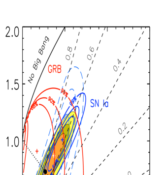
Figure 2: Constraints in the $\Omega_{\rm M}$–$\Omega_{\Lambda}$ plane derived from our GRB sample (15 objects, red contours), from the “Gold” SN Ia sample (156 objects; blue solid lines, derived assuming a fixed value of $H_{0}=65$ km s^-1 Mpc^-1, making these contours slightly different from Fig. 8 of (Riess et al. 2004), and from the subset of SNe Ia at $z>0.9$ (14 objects, blue long dashed lines). The three colored ellipses are the confidence regions (orange: 68%; light green: 90%; yellow: 99%) for the combined fit of type Ia SN+GRB samples. Dashed lines correspond to the changing sign of the cosmic acceleration [i.e. $q(z)=0$] at different redshifts, as labelled. Crosses are the centers of the corresponding contours (red: GRBs; blue: SNe Ia, white: GRB+SN Ia). The black dot marks the $\Lambda$CDM cosmology. The dotted line corresponds to the statefinder $r=1$, in this case it coincides with the flatness condition.

4 Results

For fitting the cosmological parameters we have selected the 15 GRBs reported on GGL (see §2). The GRB sample extends from $z=0.16$ to $z=3.2$. The SN Ia sample, that we combine with the GRB sample, includes the most recent discovered high redshift SNe Ia (up to 1.7) and is composed by 156 objects (the “Gold” sample, Riess et al. 2004).

For the $\Lambda$–model, we constrain $\Omega_{\rm M}$ and $\Omega_{\Lambda}$. Fig. 2 shows the confidence levels (CL) for (i) GRBs alone (adopting our Bayesian method), (ii) SNe Ia alone (for the entire “Gold” sample and for only the subset of 14 SNe Ia at $z>0.9$, using in both cases the standard approach), and (iii) the combination of all SNe Ia and GRBs. The dotted line shows the statefinder parameter $r=1$ (Sahni et al. 2003; see also the jerk parameter in Visser 2004, and Riess et al. 2004) that in $\Lambda$–model coincides with the flatness condition.

The difference between Fig. 2 and Fig. 1 of GGLF is remarkable. In Fig. 2 the most probable solution is shown by the red cross which corresponds to $\Omega_{\rm M}$=0.17 and $\Omega_{\Lambda}$=0.91, while in Fig. 1 of GGLF the best fit model corresponds to $\Omega_{\rm M}$$\simeq$0.1 and $\Omega_{\Lambda}$$\simeq$1.1.

For GRBs the CL is a little larger than for high–$z$ SNe Ia, but this CL is expected to be reduced by new experiments. Note that the orientations of the CL contours are related to the average redshift of the sample; the increase of this redshift from all SNe Ia to high–$z$ SNe Ia alone, and from high–$z$ SNe Ia to GRBs produces a counterclockwise rotation of the CL contour pattern.

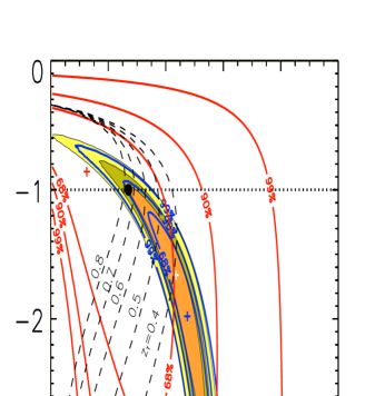
Figure 3: Constraints on $w_{0}$ and $\Omega_{\rm M}$ for a flat cosmology with dark energy whose equation of state is constant ($w_{0}=-1$ corresponds to a cosmological constant). To construct the GRB contours we have followed the same method as in Fig. 2. Colored regions: combined (GRB+SN Ia) constraints (color code as in Fig. 2). Dashed lines correspond to the changing sign of the cosmic acceleration [i.e. $q(z)=0$] at different redshifts, as labelled. Crosses are the centers of the SNe Ia contours (blue: SNe Ia alone, white: GRB+SN Ia). The black dot marks the $\Lambda$CDM cosmology. The dotted line corresponds to the statefinder $r=1$.

When we combine SNe Ia with GRBs the best–fit model moves from $\mbox{$\Omega_{\rm M}$}=0.48$, $\mbox{$\Omega_{\Lambda}$}=1.00$ for the SN Ia sample to $\mbox{$\Omega_{\rm M}$}=0.37$, $\mbox{$\Omega_{\Lambda}$}=0.87$ for the combined SN+GRB sample, favouring a closed universe. However, due to the high correlation of the CL contours in Fig. 2, the best–fit value does not mean much. Instead, it is worth to remark that the flat geometry solution $\mbox{$\Omega_{\rm M}$}+\mbox{$\Omega_{\Lambda}$}=1$ is compatible now with the 68$\%$ CL. Assuming a flat geometry prior we obtain $\mbox{$\Omega_{\rm M}$}=0.28\pm 0.03$, in excellent agreement with independent galaxy clustering measurements (Hawkins et al. 2003; Schuecker et al. 2003) and the $\Lambda$CDM cosmology. In Fig. 2 we also plot the curves of constant $z_{\rm T}$. For our best–fit model, $z_{\rm T}=0.67$, while for the flat geometry case our constraints give $z_{\rm T}=0.73\pm 0.09$.

For $W_{0}$–models Fig. 3 shows the constraints on $w_{0}$ vs $\Omega_{\rm M}$ (i.e. a constant equation of state). Best values for the SN+GRB sample are $\mbox{$\Omega_{\rm M}$}=0.44$ and $w_{0}=-1.68$ with $z_{\rm T}=0.40$, while the $\Lambda$CDM is compatible with the 68$\%$ CL (it was not for SN Ia alone). Inside the uncertainty, $w_{0}<-1$ ($r>1$) quiessence dark energy models appear favoured. However, while SN Ia best–fit model has $w_{0}<-1$, GRBs alone prefer $w_{0}>-1$, even if close to $-1$. A more complete sample of both objects is expected to support $\Lambda$CDM. For $W_{1}$–models Fig. 4 shows the constraints on the dark energy parameters $w_{0}$ vs $w^{\prime}$. For the SN+GBR sample the best–fit values are $w_{0}=-1.19$ and $w^{\prime}=0.98$ with $z_{\rm T}=0.55$. The $\Lambda$CDM again is now fully within the 68$\%$ CL of the combined SN+GRB fit. Similar to the previous case even now, inside the uncertainty, $r>1$ kinessence models (i.e. Chaplygin gas, type 1 braneworld models, see Alam et al. 2003) seem favoured. In both $W_{i}$, SN Ia alone marginally reject $\Lambda$CDM cosmology. This tendency is balanced by GRBs making hopeful a $\Lambda$CDM cosmology for the combined sample. We have here a clear example how GRBs complement the cosmological information derived by SN Ia.

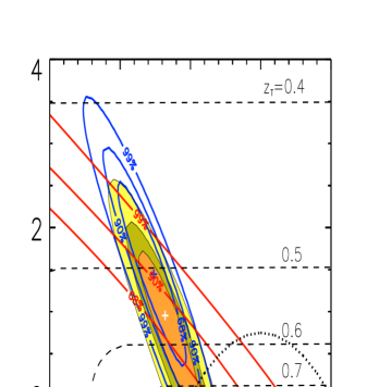
Figure 4: Constraints on the $w_{0}$ and $w^{\prime}$ parameters entering the dark energy equation of state (see §3; $w_{0}=-1$ and $w^{\prime}=0$ correspond to the cosmological constant $\Omega_{\Lambda}$). We assume a flat geometry and $\Omega_{\rm M}$=0.27. Blue contours: constraints from type Ia SNe; red contours: constraints from our GRBs. To construct the GRB contours we have followed the same method as in Fig. 2. Colored regions: combined (GRB+SN Ia) constraints (color code as in Fig. 2). Dashed lines correspond to the changing sign of the cosmic acceleration [i.e. $q(z)=0$] at different redshifts, as labelled. Crosses are the centers of the SNe Ia contours (blue: SNe Ia alone, white: GRB+SN Ia). The black dot marks the $\Lambda$CDM cosmology. Dotted line corresponds to the statefinder $r=1$.

5 Discussion

Several kinematical and dynamical parametrizations of cosmology, aimed to optimize the fittings to the available observations, have been proposed. However current Hubble diagrams of SNe Ia need to be extended to higher redshifts to constrain such parameters with better accuracy.

GRBs are the natural objects able to extend the measure of the universe to very high redshifts. This is now possible thanks to the $E_{\rm peak}$ vs. $E_{\gamma}$ empirical correlation, that allows to estimate $E_{\rm iso}$ of each GRB. At present this correlation is known on the ground of 15 GRBs distributed on redshifts up to 3.2; therefore its knowledge depends on the assumed cosmology. We presented here a new method based on a Bayesian approach that takes into account our lack of knowledge on the correlation, and optimizes the information to derive the best–fit model and the CL contours.

Despite the small number of useful GRB events and their somewhat large observational errors, a clear trend emerges when combining GRB and SNe Ia data. The inclusion of GRBs makes the $\Lambda$CDM cosmology compatible with the 68$\%$ CL. A similar trend, but less pronounced, is observed for the SN Ia sample alone when including and not the 16 HST high–$z$ SNe (see also Choudhury & Padmanabhan 2004; Alam et al. 2004).

Fig. 5 shows the Hubble diagram in the form of residuals with respect to the specific choice of $\Omega_{\rm M}$=0.27  and $\Omega_{\Lambda}$=0.73, for SNe Ia and GRBs, together with different lines corresponding to different $\Omega_{\rm M}$, $\Omega_{\Lambda}$ pairs. It is likely that the GRB event rate follows or increases with $z$ faster than the global star formation rate (e.g., Lloyd–Ronning, Fryer & Ramirez–Ruiz 2002; Yonetoku et al. 2003; Firmani et al. 2004), ensuring that GRBs exist up to $z\sim$10–20. Even at these redshifts, GRBs are easily detectable, but the ability of high–$z$ GRBs to accurately measure the Universe depends of course on the errors of the relevant observables. The fact that the bolometric fluences of GRBs with measured $z$ do not strongly correlate with $z$ (GGL) means that high–$z$ bursts can be observed with large signal-to-noise ratios. This ensures that $E_{\rm iso}$ and $E_{\rm peak}$ can be measured with good accuracy also at high $z$’s. To derive $E_{\gamma}$, we need also information related to the afterglow emission. This, for high–$z$ GRBs observed at a given time $t$ after trigger, is related to the intrinsic emission at an earlier $t/(1+z)$ time, when the emitted flux was stronger. It follows that the observed afterglow fluxes of high–$z$ GRBs are not much fainter than the afterglow fluxes of nearby GRBs observed at the same time (Lamb & Reichart 2000). Thus, high– and low–$z$ GRBs will have comparable error bars on the relevant quantities required to derive their luminosity distance. In addition, the detection of GRBs is not limited nor affected by dust extinction or by optical absorption by Ly–$\alpha$ clouds, which are instead important issues for high–$z$ SNe Ia.

Figure 5: Residuals of the distance moduli of SNe Ia and of our GRBs with respect to the $\Lambda$CDM case $\Omega_{\rm M}$=0.27, $\Omega_{\Lambda}$=0.73. Also shown are the differences of various other cosmological models with respect to the $\Omega_{\rm M}$=0.27, $\Omega_{\Lambda}$=0.73  case: red solid line: $\Omega_{\rm M}$=0.2, $\Omega_{\Lambda}$=0.8; orange solid line: $\Omega_{\rm M}$=0.37, $\Omega_{\Lambda}$=0.85; blue dot–dashed line: $\Omega_{\rm M}$=0.45, $\Omega_{\Lambda}$=0.95; black dashed line: $\Omega_{\rm M}$=1, $\Omega_{\Lambda}$=0; black dotted line: $\Omega_{\rm M}$=0.01, $\Omega_{\Lambda}$=0.99. The arrow marks the redshift of GRB 000131 ($z$=4.5) which is the most distant GRB of known $z$. Since for this GRB there is no measured jet–break time, it is not included in our sample.

References

- Alam, Sahni, & Starobinsky (2003) Alam U., Sahni V., Saini T.D. & Starobinsky A.A. 2003, preprint (astro-ph/0303009)
- Alam, Sahni, & Starobinsky (2004) Alam U., Sahni V. & Starobinsky A.A. 2004, preprint (astro-ph/0403687)
- Amati et al. (2002) Amati L. et al. 2002, A&A, 390, 81
- Bloom, Frail & Kulkarni (2003) Bloom J. S., Frail D. A. & Kulkarni S. R. 2003, ApJ, 594, 674
- Choudhury & Padmanabhan (2004) Choudhury T.R. & Padmanabhan T. 2004, preprint (astro-ph/0311622)
- Dai, Liang & Xu (2004) Dai Z.G., Liang E.W. & Xu D. 2004, ApJ, 612, L101
- (7) D’Avanzo P., et al., 2004, GCN 2788
- Dicus & Repko (2004) Dicus D.A & Repko W.W. 2004, preprint (astro-ph/0407094)
- Firmani et al. (2004) Firmani C., Avila–Reese V., Ghisellini G. & Tutukov A.V. 2004, ApJ, 611, 1033
- Frail et al. (2001) Frail D. A. et al. 2001, ApJ, 562, L55
- Galama et al. (1998) Galama T. et al. 1998, Nature 395, 670
- (12) Galassi M. et al., GCN 2770
- Ghirlanda et al. (2004a) Ghirlanda G., Ghisellini G. & Lazzati D. 2004a, ApJ, 616, 331 (GGL)
- Ghirlanda et al. (2004b) Ghirlanda G., Ghisellini G., Lazzati D. & Firmani, C. 2004b, ApJ, 613, L13 (GGLF)
- Gotz et al. (2003) Gotz D. et al. 2003, GCN 2459
- Hawkins et al. (2003) Hawkins E. et al. 2003, MNRAS, 346, 78
- Lamb & Reichart (2000) Lamb D.Q, & Reichart D.E. 2000, ApJ, 536, 1
- Linder & Huterer (2003) Linder E.V. & Huterer D. 2003, Phys. Rev. D, 67, 081303
- Lloyd-Ronning, Fryer & Ramirez-Ruiz (2002) Lloyd–Ronning N.M., Fryer C.L. & Ramirez–Ruiz E. 2002, ApJ, 574, 554
- Nesseris & Perivolaropoulos (2004) Nesseris S. & Perivolaropoulos L. 2004, preprint (astro-ph/0401556)
- Padmanabhan (2003) Padmanabhan T. 2003, Phys. Reports, 380, 235
- Peebles & Ratra (2003) Peebles P.J.E. & Ratra, B. 2003, Rev.Mod.Phys., 75, 559
- Perlmutter et al. (1999) Perlmutter S. et al. 1999, ApJ, 517, 565
- Press et al. (1999) Press W.H. et al. 1999, Numerical Recipes in C, Cambridge University Press, 661
- Riess et al. (1998) Riess A.G. et al. 1998, AJ, 116, 1009
- Riess et al. (2004) Riess A.G. et al. 2004, ApJ, 607, 665
- Rhoads (1997) Rhoads J.E. 1997, ApJL, 487, L1
- Sahni (2004) Sahni V. et al. 2004, JETP Letters 77, 201, (astro-ph/0201498)
- Sahni (2004) Sahni V. 2004, Second Aegean Summer School on the Early Universe, in press (astro-ph/0403324)
- Sari et al. (1999) Sari R., Piran T. & Halpern, J.P. 1999, ApJ, 519, L17
- Schuecker et al. (2003) Schuecker P. et al. 2003, A&A, 402, 53
- Schaefer (2003) Schaefer B.E. 2003, ApJ, 583, L67
- (33) Soderberg A. et al. 2004a, Nature, 430, 648
- (34) Soderberg A. et al. 2004b, ApJ, 606, 994
- Visser (2004) Visser M. 2004, preprint (gr-qc/0309109)
- Waxman (2004) Waxman E. 2004, ApJ, 605, L97
- Weller & Albrecht (2002) Weller J. & Albrecht A. 2002, Phys. Rev. D, 65, 103512
- Yamazaki et al. (2003) Yamazaki, R, Yonetoku D. & Nakamura T. 2003, ApJ, 594, L79
- Yonetoku et al. (2003) Yonetoku D. et al. 2003, ApJ, 609, 935