Islands in the $\Lambda$-sea: An alternative cosmological model

Abstract

We propose an alternate cosmological model in which our observable universe is an island in a cosmological constant sea. Initially the universe is filled with cosmological constant of the currently observed value but is otherwise empty. In this eternal or semi-eternal de Sitter spacetime, we show that local quantum fluctuations (upheavals) can violate the null energy condition and create islands of matter. The perturbation spectra of quantum fields other than that responsible for the upheaval, are shown to be scale invariant. With further cosmic evolution the island disappears and the local universe returns to its initial cosmological constant dominated state.

I Introduction

The last two decades have seen giant strides in observational cosmology. We now have accurate characterization of the cosmic large-scale structure, the cosmic microwave background radiation, and the energy budget of the universe. In addition we have strong support for non-baryonic dark matter, and tantalizing evidence for dark energy.

Theoretically the observations fit quite well into a cosmological framework in which a period of inflation in the earliest moments of cosmic history is postulated Guth:1980zm . The driver for inflation is a scalar field called the “inflaton” and the dynamics of the scalar field is governed by a potential function. Although there is considerable freedom to choose the scalar field content, the potential function, and initial conditions, a large number of inflationary models have been constructed that agree very well with the whole slew of observations. Most spectacular of these is the general agreement of the WMAP data with a scale invariant distribution of adiabatic density fluctuations Peiris:2003ff .

To understand the inflationary model and the generation of density fluctuations, we plot the evolution of the Hubble length scale ($H^{-1}$) in Fig. 1. The Hubble scale during inflation is a very small constant, typically of the order of $10^{3}l_{P}$ where $l_{P}\sim 10^{-33}$ cm is the Planck length. After inflation ends, cosmological reheating occurs in which the universe gets filled with radiation. From then on the universe evolves as in a Friedmann-Robertson-Walker (FRW) cosmology. Density fluctuations arise because there are quantum fluctuations in the inflationary period whose wavelengths grow during the inflationary period and eventually become larger than the Hubble scale. Once the quantum modes are superhorizon, their amplitudes are frozen. During the FRW epoch, these modes re-enter the horizon, and can give rise to the density fluctuations required for large-scale structure formation.

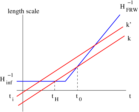
Figure 1: Sketch of the behavior of the Hubble length scale with cosmic time in inflationary cosmology, and the evolution of fluctuation modes. At early times, the vacuum energy is large and so the Hubble length scale is small and constant. Once the vacuum energy decays, inflation ends, the universe reheats and enters FRW expansion. Then the Hubble length scale grows linearly with time. The physical wavelength of a fluctuation mode starts out less than $H^{-1}_{\rm inf}$ at some early time $t_{i}$. The mode is stretched to scales larger than the horizon at some time $t_{H}(k)$. The mode later renters the horizon at some epoch $t_{0}(k)$. For illustrative purposes we have depicted that the wavelength grows linearly with cosmic time. In reality, the wavelength grows in proportion to the scale factor.

In this paper, we propose a modified cosmology which is based on a different hypothesis and investigate its viability. Instead of the evolution of the Hubble length scale shown in Fig. 1 we consider the evolution depicted in Fig. 2. We now give a short overview of the idea, explaining each stage of the model.

1. In the beginning the universe is inflating due to the observed dark energy Riess:1998cb ; Perlmutter:1998np that we assume is a cosmological constant ($\Lambda$). The de Sitter horizon size ($H^{-1}_{\Lambda}$) is comparable to our present horizon, ($H^{-1}_{0}$).

2. A quantum fluctuation of some field (e.g. scalar field, photon) in a horizon-size volume in the expanding phase of de Sitter spacetime drives the Hubble constant to a large value. Even as the Hubble length scale is decreasing the universe continues to expand. Such explosive events necessarily need to violate the null energy condition (NEC). We will show, following Refs. GutVacWin?? ; Winitzki:2001fc ; Vachaspati:2003de , that quantum field theoretic fluctuations allow for this possibility.

3. After the NEC violating fluctuation is over, the Hubble constant is large and classical radiation fills the volume. Rapid interactions thermalize the radiation. This part of the universe then evolves as a radiation dominated FRW universe and we call it an “island”.

4. With further evolution, the radiation in the FRW universe dilutes and eventually the volume is again dominated by the cosmological constant and the spacetime returns to its normal inflating state.

Our idea has elements of earlier work on eternal inflation Vilenkin:1983xq ; Linde:1986fd and especially Garriga and Vilenkin’s “recycling universe” Garriga:1997ef (see also the discussion in Carroll:2004pn ). In eternal inflation scenarios, quantum fluctuations in the inflaton field drive the Hubble length scale to smaller values. In our model we also consider a quantum fluctuation but it can occur in any quantum field and it has to be large. In both inflationary cosmology and our case, the quantum fluctuation needs to violate the NEC. Furthermore, in both cases the back-reaction of the fluctuation is assumed to lead to a faster rate of cosmological expansion. In the language of Dyson:2002pf , the evolution we are considering is one of the “miraculous” trajectories that go directly from a dead de Sitter region of spacetime to a region that is “macroscopically indistinguishable from our universe” (MIFOU). Eventually the trajectory leaves the MIFOU region and returns to the dead de Sitter region. Our idea also has elements of Steady State Cosmology BonGol48 ; Hoy48 in which matter is sporadically produced by explosive events in a hypothetical C-field but spacetime is eternal. In our case, the explosive events are quantum field theoretic and produce an entire cosmos worth of matter. The ekpyrotic cosmological model Khoury:2001wf , like our model, also utilizes a decreasing Hubble length scale. In the ekpyrotic model, the decrease in the Hubble length scale is due to extra-dimensional brane-world physics and results in a a period of contraction of our three dimensional universe. In the present model though, the Hubble length scale decreases due to an “ordinary” quantum field theoretic fluctuation, but the universe continues to expand during the contraction of the Hubble length scale.

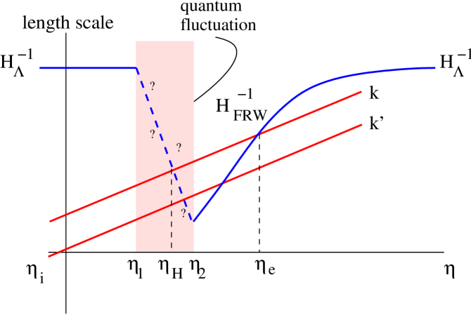
Figure 2: Sketch of the behavior of the Hubble length scale with conformal time, $\eta$, in our cosmological model, and the evolution of fluctuation modes. At early times, inflation is driven by the presently observed dark energy, assumed to be a cosmological constant. As the cosmological constant is very small, the Hubble length scale is very large – of order the present horizon size. Exponential inflation in some horizon volume ends not due to the decay of the vacuum energy as in inflationary scenarios but due to a quantum fluctuation in the time interval $(\eta_{1},\eta_{2})$ that violates the null energy condition (NEC). The NEC violating quantum fluctuation causes the Hubble length scale to decrease. After the fluctuation is over, the universe enters radiation dominated FRW expansion, and the Hubble length scale grows with time. The physical wavelength of a quantum fluctuation mode starts out less than $H^{-1}_{\Lambda}$ at some early time $\eta_{i}$. The mode exits the cosmological horizon during the NEC violating fluctuation ($\eta_{H}$) and then re-enters the horizon at some later epoch $\eta_{e}$ during the FRW epoch.

Having summarized the main idea, we now discuss each step of this model in greater detail. In Sec. VII we discuss a key test of the model – whether it predicts a scale invariant distribution of density fluctuations.

II NEC violations in de Sitter space

The first stage of the model only relies on the presence of a cosmological constant. Observations indicate some form of dark energy and they are consistent with a cosmological constant. One feature of the first stage of our model is that it does not necessarily begin in a singularity – there may be no big bang and spacetime need not be created out of nothing as in quantum cosmology. All that we need is an expanding de Sitter background and this can be part of a classical de Sitter spacetime with no beginning and no end, with early contraction and then expansion. We will only consider the expanding phase of the de Sitter spacetime in the following discussion. The scale factor of the universe at this stage is given by:

$$a(t)=a_{0}e^{H_{\Lambda}t}\equiv-\frac{1}{H_{\Lambda}\eta}$$ (1)

where $\eta\in(-\infty,0)$ is the conformal time.

In de Sitter spacetime, as well as any other spacetime, there are fluctuations of the energy-momentum tensor, $T_{\mu\nu}$, of quantum fields. This follows simply due to the fact that the vacuum, $|0\rangle$, is an eigenstate of the Hamiltonian but not of the energy-momentum density operator, ${\hat{T}}_{\mu\nu}$. In short-hand notation:

$${\hat{T}}_{\mu\nu}|0\rangle = \sum[(\dots)a_{l}a^{\dagger}_{k}+(\dots)a^{\dagger}_{l}a^{\dagger}_{k}]~{}|0\rangle$$ (2)

$$= \sum[(\dots)|0\rangle+(\dots)|2;k,l\rangle]$$

where, the ellipses within parenthesis denote various combinations of mode functions and their derivatives; $a^{\dagger}_{k}$, $a_{l}$ are creation and annihilation operators and $|2;k,l\rangle$ is a two particle state. Since the final expression is not proportional to $|0\rangle$, the vacuum is not an eigenstate of ${\hat{T}}_{\mu\nu}$ and there will be fluctuations of the energy-momentum tensor in de Sitter space.

It has been shown GutVacWin?? ; Winitzki:2001fc ; Vachaspati:2003de that quantum field theory of a light scalar field in the Bunch-Davies vacuum Bunch:1978yq in de Sitter space leads to violations of the NEC. For the present application, we only need the general arguments of Refs. GutVacWin?? ; Winitzki:2001fc ; Vachaspati:2003de and not the detailed calculations. First, one constructs the “smeared NEC operator”

$$\hat{O}^{\rm ren}_{W}\equiv\int d^{4}x\sqrt{-g}\,W\left(x;R,T\right)N^{\mu}N^{\nu}{\hat{T}}^{\rm ren}_{\mu\nu}$$ (3)

where $W\left(x;R,T\right)$ is a smearing function on a length scale $R$ and time scale $T$. The vector $N^{\mu}$ is chosen to be null, and the superscript $ren$ denotes that the operator has been suitably renormalized. By the argument given below Eq. (2) we find that ${\hat{O}}^{\rm ren}_{W}$ will fluctuate. On dimensional grounds:

$$O_{\rm rms}^{2}\equiv\langle 0|({\hat{O}}^{\rm ren}_{W})^{2}|0\rangle\sim H_{\Lambda}^{8}$$ (4)

in the special case when $R=T=H_{\Lambda}^{-1}$. Since, in de Sittter space, $\langle 0|{\hat{T}}_{\mu\nu}|0\rangle\propto g_{\mu\nu}$, we also have:

$$\langle 0|{\hat{O}}^{\rm ren}_{W}|0\rangle=0$$ (5)

Therefore the fluctuations of ${\hat{O}}^{\rm ren}_{W}$ are both positive and negative. Assuming a symmetric distribution, we come to the conclusion that quantum fluctuations of a scalar field violate the NEC with 50% probability. Exactly the same arguments can be applied to quantum fluctuations of a massless gauge field such as the photon.

The calculation described above shows that the NEC will be violated by quantum fluctuations with 50% frequency but does not give us the probability distribution of the violation amplitude. For that we would need to calculate the actual probability distribution for the operator ${\hat{O}}^{\rm ren}_{W}$. However, by continuity we can expect that large amplitude NEC violations will also occur with some diminished but non-zero probability.

III Extent and duration of NEC violation

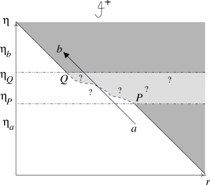
Figure 3: We show a classical de Sitter spacetime for conformal time $\eta<\eta_{P}$, that transitions to a faster expanding classical de Sitter spacetime for $\eta>\eta_{Q}$. The inverse Hubble size is shown by the white region. A bundle of ingoing null rays originating at point $a$ is convergent initially but becomes divergent in the superhorizon region at point $b$. This can only occur if the NEC is violated in the region $\eta\in(\eta_{P},\eta_{Q})$. In the quantum domain, a classical picture of spacetime may not be valid and this is made explicit by the question marks.

There are NEC violating quantum fluctuations on all spatial and temporal scales. However, most of these fluctuations are irrelevant for cosmology – the spacetime might respond very locally, and then return to its orginal state. As we now argue, only fluctuations that occur on large spatial scales can have a lasting effect on the spacetime i.e. the faster expansion can continue in a predictable way even after the NEC violating fluctuation is over.

Consider the spacetime diagram of Fig. 3. In that diagram we show an initial de Sitter space that later has a patch in which the space is again de Sitter though with a larger expansion rate. Hence the initial Hubble length scale $H_{i}^{-1}$ is larger than the final Hubble length scale $H_{f}^{-1}$. Therefore there are ingoing null rays that are within the horizon initially that propagate and are eventually outside the horizon. An example of such a null ray is the line from $a$ to $b$. At point $a$ a bundle of such rays will be converging whereas at point $b$ the bundle will be diverging. The transition from convergence to divergence of a bundle of null rays can only occur if there is NEC violation somewhere along the null ray provided some mild conditions are satisfied. This follows from the Raychaudhuri equation. In the spherically symmetric case, the mild conditions are satisfied and hence the transition to faster expansion requires NEC violation.

Now we argue that the NEC violation has to extend over a region that is at least as large as $H_{i}^{-1}$, if the faster expansion is to last longer than the duration of the NEC violation. If NEC violation only occurred on a scale smaller than $H_{i}^{-1}$, one could imagine a null ray that would never enter the NEC violating region and yet go from being converging to diverging (see Fig. 4). This would be inconsistent with the Raychaudhuri equation.

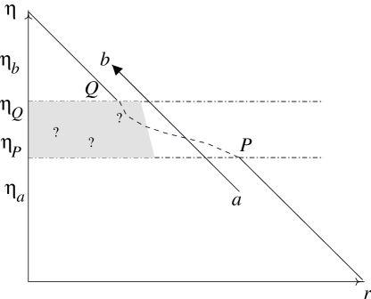
Figure 4: A spacetime diagram similar to that in Fig. 3 but one in which the NEC violation occurs over a sub-horizon region (shaded region in the diagram). Now the null ray bundle from $a$ to $b$ goes from being converging (within the horizon) to diverging (outside the horizon). However, it does not encounter any NEC violation along its path, and this is not possible as can be seen from the Raychaudhuri equation. Since the ingoing null rays are convergent as far out as the point $P$, the size of the quantum domain has to extend out to at least the inverse Hubble size of the initial de Sitter space. Therefore the NEC violating patch has to extend beyond the initial horizon.

If an NEC violation does occur in a sub-horizon region, it could cause a temporary change in the expansion rate of the region. When the NEC violating fluctuation in the small region of space ceases, the faster expanding local region would have to revert to the ambient expansion, or else some spacetime feature, such as a singularity, will have to occur that could prevent the traversal of a null ray from the slower expanding exterior region to the faster expanding interior region. Additional boundary conditions would need to be imposed at the singularity for the spacetime evolution to be predictable. An example of such a process can be found in Ref. Borde:1998wa in connection with topological inflation Vilenkin:1994pv ; Linde:1994hy .

An additional intuitive argument can be given that might help understand the need for a large spatial region where NEC is violated. Whenever a faster expanding universe is created, it must be connected by a wormhole to the ambient slower expanding region. The wormhole can be kept open if the energy conditions are violated Morris:1988cz . But, if the wormhole neck is small, as soon as the energy condition violations are over, it must collapse and pinch off into a singularity. Signals from the singularity can propagate into the faster expanding universe and predictability will be lost. However, if the neck of the wormhole is larger than the horizon size of the ambient universe, the ambient expansion can hold up the wormhole and the neck does not collapse even after the NEC violation is over.

Our argument that NEC violations on scales larger than the horizon are needed to produce a faster expanding universe is consistent with earlier work Farhi:1986ty showing that it is not possible to produce a universe in a laboratory without an initial singularity (also see Linde:1991sk ). Subsequent discussion of this problem in the quantum context Fischler:1989se ; Farhi:1989yr ; Fischler:1990pk , however, showed that a universe may tunnel from nothing without an initial singularity, just as in quantum cosmology Vilenkin:1982de ; Hartle:1983ai . In this case, the created universe is disconnected from the ambient $\Lambda$-sea. Without an inflaton, the process would therefore produce a second $\Lambda$-sea which would be empty until matter-producing fluctuations of the kind we have been discussing can create islands.

Guided by these arguments, we conjecture that small regions with finite duration NEC violation cannot lead to predictable, faster expanding islands. The conjecture is clearly not proven but we believe there is substantial evidence in favor of it. Hence we conclude that, to get a faster expanding region that lasts beyond the duration of the quantum fluctuation and remains predictable, the spatial extent of the NEC violating fluctuation must be larger than $H_{i}^{-1}$:

$$R>H_{i}^{-1}$$ (6)

where $R$ is the spatial extent of the fluctuation and shows up as the spatial smearing scale in the calculation of ${\hat{O}}_{\rm rms}$.

An explicit evaluation shows that ${\hat{O}}_{\rm rms}$ is proportional to inverse powers of the temporal smearing scale and diverges as the smearing time scale $T\rightarrow 0$. Hence the briefer the fluctuation, the stronger it can be, as we might also expect from an application of the Heisenberg time-energy uncertainty relation. Therefore we will take the time scale of the NEC violation to be vanishingly small:

$$T\rightarrow 0$$ (7)

In our analysis of the spectrum of density fluctuations in Sec. VII we will refer to this as the “sudden” approximation.

IV Backreaction on spacetime: a working hypothesis

The situation at hand has quantum fields but a classical spacetime. Generally this situation is handled using semiclassical relativity:

$$G_{\mu\nu}=8\pi G\langle{\hat{T}}_{\mu\nu}^{\rm ren}\rangle$$ (8)

where $\langle\rangle$ denotes the expectation value in some specified quantum state. Hence the spacetime in this formalism only responds to the expectation value of the energy-momentum tensor and fluctuations about the mean do not play any role. However we are interested in precisely the effects of fluctuations of ${\hat{T}}_{\mu\nu}^{\rm ren}$ and so it is essential that we go beyond semiclassical relativity to be able to treat the backreaction of the NEC violating fluctuations on the spacetime. For small fluctuations, one could envisage expanding the metric around a fixed background and quantizing the metric fluctuations. Such an attempt has been made in Refs. Tsamis:1996qm though not in the context of NEC violations. The perturbative scheme can not however hope to capture the physics of large fluctuations of the kind we are interested in.

Since a rigorous treatment of the backreaction is not possible, we shall adopt a “working hypothesis” in which the NEC violating fluctuation behaves like “phantom energy” i.e. a classical perfect fluid with equation of state $w\equiv p/\rho<-1$ where $\rho>0$. Furthermore, in the sudden approximation discussed in the previous section, the phantom energy exists only for a vanishingly small time period. Hence the energy content of the universe has the following time dependence:

$$\rho=\Lambda\ ,\ \ w=-1\ ,\ \ \eta<\eta_{f}$$

$$\rho=\rho_{\rm FRW}\ ,\ \ w=+\frac{1}{3}\ ,\ \ \eta>\eta_{f}$$ (9)

where $\eta_{f}$ denotes the instant at which the NEC violating fluctuation occurs and $\rho_{\rm FRW}$ denotes the energy density after the NEC violating fluctuation is over and this is assumed to be dominantly in the form of radiation. The initial condition for the FRW phase is: $\rho_{\rm FRW}(\eta_{f})=\rho_{\rm mg}$, the radiation density required for matter-genesis.

With this working hypothesis for the energy content of the local universe, the backreaction on the spacetime is given by:

$$H^{2}=\frac{8\pi G}{3}\rho$$ (10)

where, as usual, $H={\dot{a}}/a$ and $a(t)$ is the local scale factor. For $\eta<\eta_{f}$, $\rho$ is a constant and $H=H_{\Lambda}$ which is constant. In a vanishingly small interval around $\eta_{f}$, $\rho$ increases rapidly due to the NEC violating fluctuation and this means that $H$ also increases correspondingly. This implies that the scale factor grows faster than exponentially during the NEC violating fluctuation, yielding a vanishingly short period of “super-inflation”. After the NEC violating fluctuation is over, the region is filled with radiation energy density and the FRW epoch starts. We summarize the behavior of the Hubble scale, $H$, as follows:

$$H=H_{\Lambda}\ ,\ \ \eta<\eta_{f}$$

$$H=H_{\rm FRW}\ ,\ \ \eta>\eta_{f}$$ (11)

with the initial condition $H_{\rm FRW}(\eta_{f})=H_{mg}$ where $H_{mg}$ is the Hubble constant at the epoch of matter-genesis.

In writing Eq. (10), we are assuming that spacelike surfaces of constant $\rho$ are flat. That is why we have not included the spatial curvature term, $k/a^{2}$. This is consistent with our working hypothesis since the initial state ($\eta<\eta_{f}$) is flat and the universe expands even faster during the phantom energy stage which is entirely classical. In the oft studied example where a scalar field tunnels through to a different value, it is known that the surfaces of constant field have negative spatial curvature. The energy density in the field is purely due to potential energy and so the surfaces of constant field are also surfaces of constant energy density. Hence the tunneling event produces an open universe with negative spatial curvature Bucher:1994gb . The scenario in this paper is different from the tunneling scenario because there is no instanton that describes the NEC violating fluctuation. It can be shown explicitly that the tunneling process preserves de Sitter invariance Vachaspati:1991tq (though see the caveat mentioned in Footnote 33 in Vilenkin:1994rn ) and this symmetry implies hyperbolic spatial slicings (i.e. open universe slicings) of the spacetime. In our case we know that NEC violations only occur if de Sitter invariance is broken. This can be seen by considering

$$\langle{\hat{T}}_{\mu\nu}^{\rm ren}{\hat{T}}_{\lambda\sigma}^{\rm ren}\rangle$$ (12)

If we demand that this be a tensor respecting the de Sitter symmetry, then it must be expressible in terms of the metric tensor since this is the only tensor available to us. However, then, when we contract with null vectors to get $\langle(N^{\mu}N^{\nu}{\hat{T}}_{\mu\nu}^{\rm ren})^{2}\rangle$, the result will be zero since $g_{\alpha\beta}N^{\alpha}N^{\beta}=0$, and there will be no NEC violating fluctuations.

The smearing process that is used in the calculation of $O_{\rm rms}$ is essential in quantum field theory since quantum operators are distributions that are defined solely by their actions on test functions, much like the Dirac delta function (see Chapter 3 of StrWig64 ). Therefore only the smeared operator ${\hat{O}}_{W}^{\rm ren}$ has physical meaning and it explicitly breaks de Sitter invariance. The fluctuations of ${\hat{O}}_{W}^{\rm ren}$ depend on the spacetime volume under consideration.

In the preceding sections we have described the nature of the fluctuation and a working hypothesis for determining the backreaction of the fluctuation on the spacetime. We now discuss the likelihood of getting the described NEC violating fluctuation.

V Likelihood – the role of the observer

In Sec. III we have seen that a cosmologically relevant NEC violation must occur on superhorizon scales and will most likely be on very short time scales. Even among such fluctuations, most of the NEC violating fluctuations will be small in magnitude. The energy density produced as a result of small fluctuations will also be small and will not impact observational cosmology. However, there is a tiny probability of having a large fluctuation in which there is sufficient energy density to heat a horizon-size volume to a very high temperature. If the temperature produced is high enough, matter-genesis will occur in this region eventually leading to large-scale structure and to the cosmology we observe. If the temperature is not high enough for matter-genesis, the island of energy will not lead to a matter dominated cosmology of the kind we know. We are assuming that matter-genesis is essential for observers to exist.

A large NEC violating fluctuation in which an island of matter is produced is very improbable. However, since spacetime is eternal in this model we can wait indefinitely for the island of matter to be produced. The island of matter can then proceed to thermalize, cool and form our present day cosmic environment. We also assume that the temperature required for magnetic monopoles production is higher than that required for matter-genesis. If the temperature at the beginning of the FRW phase is below that needed for monopole formation but above the matter-genesis temperature then there will be no cosmological magnetic monopole problem. This solution to the monopole over-abundance problem is similar in spirit to that proposed in Ref. Dvali:1995cj where the Grand Unified phase transition never occurs.

The probability of fluctuations in the $\Lambda$-sea that can lead to an inflating cosmology versus those that produce an FRW universe have been considered by several researchers Dyson:2002pf ; Albrecht:2004ke . In particular, Dyson et al. Dyson:2002pf estimate probabilities based on a “causal patch” picture, with the conclusion that it is much more probable to directly create a universe like ours than to arrive at our present state via inflation. Albrecht and Sorbo Albrecht:2004ke have argued that the conclusion rests crucially on the causal patch picture, and provide a different calculation leading to the conclusion that inflationary cosmology is favored. Both calculations assume the existence of fields that are suitable for inflation. In this case, one should also include the additional possibility of “creating a universe from nothing” in the evaluation of relative probabilities.

Our hypothesis is that there exists no field that is suitable to be an inflaton. So the comparison of the likelihood of inflation versus no inflation is moot. What is still relevant is the relative probability of obtaining an island which is different from ours but those in which observers could live. We do not know the various necessary conditions for life. However, once we have assumed that the end point of the NEC violating fluctuation is a thermal state with all the different forms of matter in thermal equilibrium, further evolution of the island simply follows that of standard big bang cosmology.

In island cosmology, we need also ask where we are located on the island. Are we close to the edge of the island (“beach”)? In that case we would observe anisotropies in the cosmic microwave background since in some directions we would see the $\Lambda$-sea while in others we would see inland. However, the island is very large (by a factor $a_{0}/a_{f}$) compared to our present horizon, $H_{\Lambda}^{-1}$. If we assume a uniform probability for our location on the island, our distance from the $\Lambda$-sea will be an $O(1)$ fraction of $H_{\Lambda}^{-1}a_{0}/a_{f}$. Since $a_{0}/a_{f}$ is of order $T_{mg}/T_{0}$ – the ratio of the matter-genesis temperature to the present temperature – we are most likely to be sufficiently inland so as not to observe any anisotropy in the cosmic microwave background.

Whereas inflationary models crucially rely on the existence of a suitable scalar field (inflaton), we have so far not specified the quantum field that causes the NEC violating fluctuation. We now turn to this issue.

VI The NEC violating field

The phantom energy that is assumed to describe the effects of the NEC violating quantum fluctuation, by definition, satisfies $\rho+p<0$. In addition, the assumption that the backreaction is given by Eq. (10), requires $\rho>0$. Hence we need a quantum field that can give NEC violating fluctuations while still having positive energy density. In other words, the energy density should be positive but the pressure should be sufficiently negative so that the NEC is violated.

First consider a scalar field, $\phi$, with potential $V(\phi)$. The energy density and pressure are:

$${\hat{\rho}} = \frac{1}{2}{\dot{\phi}}^{2}+\frac{1}{2}({\bm{\nabla}}\phi)^{2}+V(\phi)$$

$${\hat{p}} = \frac{1}{2}{\dot{\phi}}^{2}-\frac{1}{6}({\bm{\nabla}}\phi)^{2}-V(\phi)$$ (13)

where the hats on $\rho$ and $p$ emphasize that these are quantum operators Therefore:

$${\hat{\rho}}+{\hat{p}}={\dot{\phi}}^{2}+\frac{({\bm{\nabla}}\phi)^{2}}{3}$$ (14)

The operators ${\hat{\rho}}$ and ${\hat{\rho}}+{\hat{p}}$ are not proportional to each other and fluctuations in one do not have to be correlated with fluctuations of the other. The energy density in a region can be positive while the NEC is violated. Therefore a scalar field, even if $V(\phi)=0$, can provide suitable NEC violating fluctuations.

The particle physics in the very early stages of the model is described by low energy particle physics that we know so well. At present we do not have any experimental evidence for a scalar field. One field that we know of today is the electromagnetic field. Could the electromagnetic field give rise to a suitable NEC violating fluctuation?

For the electromagnetic field we have:

$${\hat{\rho}}=\frac{1}{2}({\bf E}^{2}+{\bf B}^{2})$$

$${\hat{p}}=\frac{1}{6}({\bf E}^{2}+{\bf B}^{2})=\frac{1}{3}{\hat{\rho}}$$ (15)

So now ${\hat{\rho}}$ and ${\hat{p}}$ are not independent operators and

$${\hat{\rho}}+{\hat{p}}=\frac{4}{3}{\hat{\rho}}$$ (16)

From this relationship between the operators, it is clear that the only electromagnetic fluctuation that can violate the NEC also has negative energy density. This means that even though the electromagnetic field can violate the NEC, it does not satisfy the positive energy density condition needed in the working hypothesis to find the backreaction. It may be possible that the electromagnetic field will still be found to be suitable once we know better how to handle the backreaction problem. Then perhaps we will not need to rely on the working hypothesis that requires positive energy density.

There is a possible loophole in our discussion of the electromagnetic field. The equation of state ${\hat{p}}={\hat{\rho}}/3$ follows from the conformal invariance of the electromagnetic field ${\hat{T}}^{\mu}_{\mu}=0$. However, we know that quantum effects in curved spacetime give rise to a conformal anomaly and the trace $\langle{\hat{T}}^{\mu}_{\mu}\rangle$ is not precisely zero. So we can expect that the equation of state ${\hat{p}}={\hat{\rho}}/3$ is also anomalous. Whether this anomaly can allow for NEC violations with positive energy density is not clear to us.

Note that it is not necessary for the NEC violation to originate from a fluctuation of a massless or light field. The arguments of Sec. II are very general and apply to massive fields as well. Though, for a massive field, ${\hat{O}}_{\rm rms}$ will be further suppressed by exponential factors whose exponent depends on powers of $H_{\Lambda}/m$. While the likelihood of a suitable NEC violating flucutation from a very massive field is much smaller compared to that of a light or massless field, the massive field fluctuations are clearly more important if the light field doesn’t even exist! The discussion in the previous section of the likelihood still applies.

VII Spectrum of perturbations

In contrast to inflationary models, we do not have a classical field that is slowly rolling on some potential. Instead a mode of a field (call it $\phi$) is undergoing an NEC violating quantum fluctuation. In general there will also be quantum fluctuations of the other modes of the field and these will give rise to density fluctuations. In addition to fluctuations of $\phi$, there will be other fields that will undergo quantum fluctuations in the rapidly changing spacetime and these will also give rise to density fluctuations. Some of these will be massless or light compared to $H_{\Lambda}$ and for others the mass will be important. However, we might expect that the mass will be important only if it is larger than the final value of the Hubble parameter after the fluctuation is over, denoted by

$$H_{f}\equiv H(\eta_{f}+)$$ (17)

We will not pursue massive fields further but restrict our attention to massless fields for the present.

First we will consider a light field other than $\phi$, and not interacting directly with $\phi$, and find its power spectrum. Let us denote such a field generically by $\chi$, its eigenmodes by $\chi_{k}(\eta)\exp(i{\bf k}\cdot{\bf x})$ and, as is commonly done in the theory of cosmological perturbations Mukhanov:1990me , define the variable

$$v_{k}(\eta)\equiv a(\eta)\chi_{k}(\eta)$$ (18)

with $k=|{\bf k}|$. If $\chi$ is a massless, minimally coupled scalar field then $v_{k}$ satisfies:

$$v_{k}^{\prime\prime}+\biggl{(}k^{2}-\frac{a^{\prime\prime}}{a}\biggr{)}v_{k}=0$$ (19)

where primes denote differentiation with respect to the conformal time $\eta$ ($dt=ad\eta$). The solution of Eq. (19) with suitable initial conditions (described below) directly leads to the power spectrum of $\chi$ perturbations at any time via:

$${\cal P}_{\chi}(k,\eta)=\frac{k^{3}}{2\pi^{2}}\left|\frac{v_{k}}{a}\right|^{2}$$ (20)

In the de Sitter phase of the cosmology, i.e. for $\eta<\eta_{f}$,

$$\frac{a^{\prime\prime}}{a}=\frac{2}{\eta^{2}}$$ (21)

The exact solution of Eq. (19) with the boundary condition that small wavelength modes go over into Minkowski space modes is:

$$v_{k}=\frac{e^{-ik\eta}}{\sqrt{2k}}\left(1-\frac{i}{k\eta}\right)\ ,\ \ \eta<\eta_{f}$$ (22)

The other independent mode is $v_{k}^{*}$. These are the mode functions for the Bunch-Davies vacuum Bunch:1978yq . A derivation of these mode functions using inverse scattering technology can be found in the Appendix.

In the radiation dominated FRW epoch, i.e. for $\eta>\eta_{f}$, we have

$$a(t)=a_{f}\sqrt{\frac{t}{t_{f}}}$$ (23)

where $t_{f}$ is the cosmic time at which the NEC violating fluctuation occurs, and $a_{f}\equiv a(t_{f})$. (Note that the Hubble parameter is discontinuous at $\eta_{f}$ in the sudden approximation but the scale factor is continuous.) In terms of the conformal time one finds:

$$a(\eta)=a_{f}+a_{f}^{2}H_{f}(\eta-\eta_{f})$$ (24)

Clearly $a^{\prime\prime}=0$. Therefore:

$$v_{k}=\alpha_{k}e^{-ik\tau}+\beta_{k}e^{+ik\tau}\ ,\ \ \tau\equiv\eta-\eta_{f}>0$$ (25)

Next we need to solve Eq. (19) at $\eta=\eta_{f}$. This step is non-trivial since $a$ is continuous at $\eta_{f}$ but $a^{\prime}$ is discontinuous. Hence $a^{\prime\prime}$ has a delta function contribution. Using Eqs. (1) and (24) we find:

$$\frac{a^{\prime\prime}}{a}=\frac{2}{\eta^{2}}\Theta(\eta_{f}-\eta)+a_{f}\Delta H\delta(\eta-\eta_{f})$$ (26)

where $\Theta(\cdot)$ is the Heaviside function and

$$\Delta H\equiv H_{f}-H_{\Lambda}\approx H_{f}$$ (27)

Integrating Eq. (19) in an infinitesimal interval around $\eta_{f}$, we find the junction conditions:

$$v_{k}(\eta_{f}+) = v_{k}(\eta_{f}-)$$

$$v_{k}^{\prime}(\eta_{f}+) = v_{k}^{\prime}(\eta_{f}-)+a_{f}\Delta Hv_{k}(\eta_{f})$$ (28)

where the last term is due to the $\delta-$function piece in $a^{\prime\prime}/a$. We can now find the coefficients $\alpha_{k}$ and $\beta_{k}$ by inserting the de Sitter and FRW mode functions and their derivatives at $\eta=\eta_{f}$ in the junction conditions. This gives:

$$\alpha_{k}=\frac{1}{2}\left[v_{kf-}+\frac{i}{k}\biggl{(}v_{kf-}^{\prime}+a_{f}H_{f}v_{kf-}\biggr{)}\right]$$

$$\beta_{k}=\frac{1}{2}\left[v_{kf-}-\frac{i}{k}\biggl{(}v_{kf-}^{\prime}+a_{f}H_{f}v_{kf-}\biggr{)}\right]$$ (29)

where $v_{kf-}\equiv v_{k}(\eta_{f}-)$ and similarly for the (conformal) time derivative $v_{k}^{\prime}$.

We are interested in the long wavelength fluctuations for which $k\eta_{f}\rightarrow 0$. Then the dominant contributions come from the $v_{kf-}^{\prime}$ and $a_{f}H_{f}v_{kf-}$ terms in Eq. (29) and are of order $1/(k\eta_{f})^{2}$. However, the $a_{f}H_{f}v_{kf-}$ term is much larger than the $v_{kf-}$ term because $H_{f}>>H_{\Lambda}$. (Recall from Eq. (1) that $a_{f}\eta_{f}=-1/H_{\Lambda}$.) Therefore

$$\alpha_{k} \approx +\frac{1}{2\sqrt{2k}}\frac{1}{(k\eta_{f})^{2}}\frac{H_{f}}{H_{\Lambda}}$$

$$\beta_{k} \approx -\frac{1}{2\sqrt{2k}}\frac{1}{(k\eta_{f})^{2}}\frac{H_{f}}{H_{\Lambda}}$$ (30)

Therefore

$$v_{k}(\eta)\approx\frac{-i}{\sqrt{2k}}\frac{1}{(k\eta_{f})^{2}}\frac{H_{f}}{H_{\Lambda}}\sin(k\eta)$$ (31)

Using Eqs. (24) and (31) in (20), together with $\eta_{k}>>\eta_{f}$ gives:

$${\cal P}_{\chi}(k,\eta_{k})\approx\frac{1}{4\pi^{2}}\frac{1}{a_{f}^{4}H_{\Lambda}^{2}\eta_{f}^{4}}\biggl{(}\frac{\sin(k\eta)}{k\eta}\biggr{)}^{2}$$ (32)

Making use of Eq. (1), $a_{f}\eta_{f}=-1/H_{\Lambda}$, and taking the limit $k\eta\rightarrow 0$, we finally get:

$${\cal P}_{\chi}(k,\eta_{k})\approx\frac{H_{\Lambda}^{2}}{4\pi^{2}}$$ (33)

Since the result does not depend on $k$, the spectrum of $\chi$ fluctuations is scale invariant, as in the inflationary case MukChi81 , with amplitude set by the cosmological constant.

As discussed earlier in this section, the result in Eq. (33) applies to all very light or massless fields other than, and not interacting directly with, the NEC violating field. In particular, in the context of the gravitational wave power spectrum, the perturbation of the metric is equivalent to $\chi/m_{P}$ where $m_{P}$ is the Planck mass. Hence the power in gravitational waves is proportional to $(H_{\Lambda}/m_{P})^{2}$ and is very tiny.

We now turn to the problem of estimating fluctuations of the NEC violating field itself. The NEC violating field (called $\phi$) is decomposed in a part that is responsible for the fluctuation ($\phi_{0}$) and another ($\delta\phi$) that takes into account additional small fluctuations. Hence we write:

$$\phi=\phi_{0}+\delta\phi$$ (34)

where, in contrast to the inflationary case, both $\phi_{0}$ and $\delta\phi$ are quantum operators.

To calculate density fluctuations due to $\delta\phi$, one needs a suitable model for the evolution of $\phi_{0}$ during the NEC violating fluctuation. This evolution is quantum and not described as a solution to some classical equation of motion. The closest related problems that have been addressed in the literature are the production of particles during the quantum creation of the universe and the fluctuations of a vacuum bubble that has itself been produced in a tunneling event Rubakov:1984pa ; Vachaspati:1991tq ; Garriga:1991tb . These analyses rely on the existence of an instanton describing the tunneling event. In our case, the NEC violation is not described by an instanton; instead it is described by the most probable fluctuation leading to matter-genesis. Hence the existing techniques do not apply directly and new techniques are needed. We leave this as an open problem for future work.

VIII Assumptions

Island cosmology involves several assumptions that we have pointed out above but now summarize and discuss.

Our first assumption is that the dark energy is a cosmological constant. This is consistent with observations and moreover is the simplest explanation of the Hubble acceleration. We assume that the cosmological constant provides us with a background de Sitter spacetime that is eternal. As de Sitter spacetime also has a contracting phase, the singularity theorems of Ref. Borde:2001nh are evaded.

The second assumption is that there is a scalar field in the model responsible for the NEC violation. It would have been more satisfactory if the electromagnetic field could have played this role but we have shown (up to the loophole of the conformal anomaly) that the conformal invariance of the electromagnetic field prevents NEC violations with positive energy density. It is possible that with a better understanding of the backreaction of quantum energy-momentum fluctuations on the spacetime, the electromagnetic field might still provide suitable NEC violations (see Sec. IV).

The basic formalism of quantum field theory in curved spacetime clearly leads to NEC violations and this is not an assumption. (Though one could reasonably question the applicability of quantum field theory on systems with horizons.) Then there seems little doubt that there should exist large amplitude NEC violations, though occurring much more infrequently than the small amplitude violations. The idea that NEC violating fluctuations could have played an important cosmological role is also to be found in the “eternal inflation” scenario Borde:1997pp . Indeed, the current scenario may also be viewed as an eternal inflation scenario – since the universe is eternally inflating due to a cosmological constant! While we may not be able to test the idea of cosmological NEC violating fluctuations, we can certainly test quantum fluctuations with and without horizons in laboratory experiments Unruh:1980cg ; Fischer:2004bf ; Jacobson:1998he ; Vachaspati:2004wn .

The third assumption we have made has to do with NEC violations in regions of small spatial extent. Based on work done on the possibility of creating a universe in a laboratory, topological inflation, and wormholes, we have argued for the conjecture that small scale violations of NEC can only give rise to universes that are affected by signals originating at a singularity. Hence predictability is lost in such universes. Our assumption is that even if we did know how to handle the spacetime singularities affecting these universes, they would turn out to be unsuitable for matter genesis. Without this assumption, we should also be considering such universes as possible homes.

The fourth assumption is that the final state of the fluctuation is a thermal state. All the different energy components are also assumed to be in thermal equilibrium. We have then assumed that the critical temperature needed for observers to exist is the temperature at which matter-genesis occurs. One could relax this assumption but one would need an adequate characterization of the most likely state to be able to calculate cosmological observables (e.g. spectrum of density fluctuations).

Our fifth assumption is our “working hypothesis” for the backreaction of the NEC violating fluctuation. This seems to be the weakest assumption in our analysis. However, we cannot do any better at the moment because the backreaction of quantum fluctuations on the spacetime requires that we consider a quantum theory of gravity as well. The backreaction problem also occurs in eternal inflationary cosmology where a similar working hypothesis is used. It would be worthwhile to address the issue of backreaction using quantum cosmology, string theory, or loop gravity, but that project is beyond the scope of this paper.

This brings us to the part of the model where we argue that even if the large amplitude fluctuations are infrequent, they are the only ones that are relevant for observational cosmology. This is quite similar to the arguments given in the context of eternal inflationary cosmology where thermalized regions are relatively rare but these are the only habitable ones. It also occurs in chaotic inflation Linde:1983gd , where closed universes of all sizes and shapes are produced but only a few are large and homogeneous enough to develop into the present universe. So this part of our model is no weaker (and harder to quantify) than other cosmological models.

IX Conclusions

To conclude, we have investigated a new cosmological model, which we call “island cosmology”, where large NEC violating quantum fluctuations (“upheavals”) in a cosmological constant de Sitter universe create islands of matter. In island cosmology, spacetime may be non-singular and eternal. We have shown that fields other than the NEC violating field yield a scale invariant spectrum of perturbations.

The spectrum of density perturbations due to the NEC violating field itself is left as an open problem. Determining this spectrum will be crucial to determining if the model agrees with observations. For example, if the scale of fluctuations in this field is still set by $(H_{\Lambda}/m_{P})^{2}$ then the fluctuations are too small to seed the structure that we know and the island will be a desert. On the other hand, if the scale is set by $(H_{f}/m_{P})^{2}$ then there is a chance that island cosmology can be a viable model. In that case, quantum NEC violations provide a definite mechanism by which regions that are “macroscopically indistinguishable from our universe” can be produced from the dead de Sitter sea.

Suppose the spectrum of density fluctuations in island cosmology turns out to agree with observations. Then the question would arise if we can somehow distinguish island cosmology from an inflationary scenario that is also consistent with observations. Unfortunately the answer seems to be that no cosmological observation can distinguish between the scenarios because of the immense adaptability of inflationary models. The only distinguishing feature would have to come from the field theory side since island cosmology does not rely on constructing a suitable potential for a scalar field whereas this seems to be a crucial feature in inflationary models. If the electromagnetic field is subsequently determined to be capable of providing suitable NEC violations, scalar fields might be dispensed off entirely in island cosmology.

The flip side of island cosmology is that if the density fluctuations turn out not to agree with observations, we can dismiss the scenario of our universe being an island in the $\Lambda$-sea, even though quantum field theory predicts the existence of such islands. This in itself would be an interesting conclusion.

Appendix A Solution for the de Sitter mode functions

Here we will solve the mode function equation based on a technique encountered in the inverse scattering literature (for example, see Ref. Kwong:1985ti ).

The differential equation we wish to solve, Eq. (19), can be written as:

$$-v_{k}^{\prime\prime}+\frac{a^{\prime\prime}}{a}v_{k}=k^{2}v_{k}$$ (35)

which is a Schrodinger equation with potential $a^{\prime\prime}/a$ and eigenvalue $k^{2}$. Now

$$\frac{a^{\prime\prime}}{a}=f^{\prime}+f^{2}$$ (36)

where $f\equiv a^{\prime}/a$. Therefore the Hamiltonian is:

$$H=-\partial^{2}+f^{\prime}+f^{2}=(\partial+f)(-\partial+f)$$ (37)

Denoting

$$Q=-\partial+f\ ,\ \ Q^{+}=\partial+f$$ (38)

we can write:

$$H=Q^{+}Q$$ (39)

Therefore the original differential equation is:

$$Q^{+}Qv_{k}=k^{2}v_{k}$$ (40)

Now consider the “partner” Hamiltonian:

$$H_{-}=QQ^{+}=-\partial^{2}-f^{\prime}+f^{2}$$ (41)

and consider the partner Schrodinger equation:

$$QQ^{+}u_{E}=Eu_{E}$$ (42)

Claim: if $u_{E}$ is a solution to Eq. (42) then $v_{k}=Q^{+}u_{E}$ is a solution to Eq. (40) with $k^{2}=E$. This claim is easy to check since:

$$Hv_{k}=Q^{+}Q(Q^{+}u_{E})=Q^{+}H_{-}u_{E}=Ev_{k}$$ (43)

This result is useful because if we know the eigenstates of the partner Schrodinger equation, we can find the eigenstates of the original Hamiltonian by applying $Q^{+}=\partial+f$ to the partner eigenstate.

In the case of mode functions in de Sitter space ($a=-1/H\eta$),

$$f=\frac{a^{\prime}}{a}=-\frac{1}{\eta}$$ (44)

and hence

$$H_{-}=-\partial^{2}-f^{\prime}+f^{2}=-\partial^{2}$$ (45)

Since this is the Hamiltonian for modes in Minkowski space, we observe that the de Sitter and Minkowski Hamiltonians are partners.

The eigenstates of $H_{-}$ are:

$$u_{k}=\frac{C_{k}}{\sqrt{2k}}e^{-ik\eta}$$ (46)

where $C_{k}$ is a normalization factor, with $k$ being any real number. Therefore

$$v_{k}=Q^{+}u_{k}=(-ikC_{k})\frac{e^{-ik\eta}}{\sqrt{2k}}\left(1-\frac{i}{k\eta}\right)$$ (47)

The correctly normalized mode function is obtained with $-ikC_{k}=1$.

This technique can be applied to the case of a massive scalar field too where the solutions are known in terms of Hankel functions. While the solution is not as simple, the technique enables us to find a relation between mode functions for two different parameters.

References

- (1) A. H. Guth, Phys. Rev. D 23, 347 (1981).
- (2) H. V. Peiris et al., Astrophys. J. Suppl. 148, 213 (2003) [arXiv:astro-ph/0302225].
- (3) A. G. Riess et al. [Supernova Search Team Collaboration], Astron. J. 116, 1009 (1998) [arXiv:astro-ph/9805201].
- (4) S. Perlmutter et al. [Supernova Cosmology Project Collaboration], Astrophys. J. 517, 565 (1999) [arXiv:astro-ph/9812133].
- (5) A. Guth, T. Vachaspati and S. Winitzki, unpublished.
- (6) S. Winitzki, arXiv:gr-qc/0111109.
- (7) T. Vachaspati, arXiv:astro-ph/0305439.
- (8) A. Vilenkin, Phys. Rev. D 27, 2848 (1983).
- (9) A. D. Linde, Phys. Lett. B 175, 395 (1986).
- (10) J. Garriga and A. Vilenkin, Phys. Rev. D 57, 2230 (1998) [arXiv:astro-ph/9707292].
- (11) S. M. Carroll and J. Chen, arXiv:hep-th/0410270.
- (12) L. Dyson, M. Kleban and L. Susskind, JHEP 0210, 011 (2002) [arXiv:hep-th/0208013].
- (13) H. Bondi and T. Gold, Mon. Not. Roy. Astron. Soc., 108, 252 (1948)
- (14) F. Hoyle, Mon. Not. Roy. Astron. Soc., 108, 372 (1948); ibid., 109, 365 (1949).
- (15) J. Khoury, B. A. Ovrut, P. J. Steinhardt and N. Turok, Phys. Rev. D 64, 123522 (2001) [arXiv:hep-th/0103239].
- (16) T. S. Bunch and P. C. W. Davies, Proc. Roy. Soc. Lond. A 360, 117 (1978).
- (17) T. Vachaspati and M. Trodden, Phys. Rev. D 61, 023502 (2000) [arXiv:gr-qc/9811037].
- (18) A. Borde, M. Trodden and T. Vachaspati, Phys. Rev. D 59, 043513 (1999) [arXiv:gr-qc/9808069].
- (19) A. Vilenkin, Phys. Rev. Lett. 72, 3137 (1994) [arXiv:hep-th/9402085].
- (20) A. D. Linde, Phys. Lett. B 327, 208 (1994) [arXiv:astro-ph/9402031].
- (21) E. Farhi and A. H. Guth, Phys. Lett. B 183, 149 (1987).
- (22) A. D. Linde, Nucl. Phys. B 372, 421 (1992) [arXiv:hep-th/9110037].
- (23) W. Fischler, D. Morgan and J. Polchinski, Phys. Rev. D 41, 2638 (1990).
- (24) E. Farhi, A. H. Guth and J. Guven, Nucl. Phys. B 339, 417 (1990).
- (25) W. Fischler, D. Morgan and J. Polchinski, Phys. Rev. D 42, 4042 (1990).
- (26) A. Vilenkin, Phys. Lett. B 117, 25 (1982).
- (27) J. B. Hartle and S. W. Hawking, Phys. Rev. D 28, 2960 (1983).
- (28) M. S. Morris and K. S. Thorne, Am. J. Phys. 56, 395 (1988).
- (29) N. C. Tsamis and R. P. Woodard, Annals Phys. 253, 1 (1997) [arXiv:hep-ph/9602316].
- (30) M. Bucher, A. S. Goldhaber and N. Turok, Phys. Rev. D 52, 3314 (1995) [arXiv:hep-ph/9411206].
- (31) T. Vachaspati and A. Vilenkin, Phys. Rev. D 43, 3846 (1991).
- (32) A. Vilenkin, Phys. Rev. D 50, 2581 (1994) [arXiv:gr-qc/9403010].
- (33) R.F. Streater and A.S. Wightman, “PCT, Spin and Statistics, and All That”, W.A. Benjamin, New York (1964).
- (34) G. R. Dvali, A. Melfo and G. Senjanovic, Phys. Rev. Lett. 75, 4559 (1995) [arXiv:hep-ph/9507230].
- (35) A. Albrecht and L. Sorbo, Phys. Rev. D 70, 063528 (2004) [arXiv:hep-th/0405270].
- (36) V. F. Mukhanov, H. A. Feldman and R. H. Brandenberger, Phys. Rept. 215, 203 (1992).
- (37) V.F. Mukhanov and G.V. Chibisov, JETP Lett. 33, No. 10, 532 (1981); reprinted in astro-ph/0303077.
- (38) V. A. Rubakov, Nucl. Phys. B 245, 481 (1984).
- (39) J. Garriga and A. Vilenkin, Phys. Rev. D 45, 3469 (1992).
- (40) N. Goheer, M. Kleban and L. Susskind, JHEP 0307, 056 (2003) [arXiv:hep-th/0212209].
- (41) A. Borde, A. H. Guth and A. Vilenkin, Phys. Rev. Lett. 90, 151301 (2003) [arXiv:gr-qc/0110012].
- (42) A. Borde and A. Vilenkin, Phys. Rev. D 56, 717 (1997) [arXiv:gr-qc/9702019].
- (43) W. G. Unruh, Phys. Rev. Lett. 46, 1351 (1981).
- (44) U. R. Fischer and R. Schutzhold, Phys. Rev. A 70, 063615 (2004) [arXiv:cond-mat/0406470].
- (45) T. A. Jacobson and G. E. Volovik, Pisma Zh. Eksp. Teor. Fiz. 68, 833 (1998) [JETP Lett. 68, 874 (1998)] [arXiv:gr-qc/9811014].
- (46) T. Vachaspati, J. Low Temp. Phys. 136, Nos. 5/6 (2004) [arXiv:cond-mat/0404480].
- (47) A. D. Linde, Phys. Lett. B 129, 177 (1983).
- (48) W. Kwong and J. L. Rosner, Prog. Theor. Phys. Suppl. 86, 366 (1986).