The structure of the Galactic bar

Abstract

We present a deep near-infrared wide-angle photometric analysis of the structure of the inner Galactic bar and central disk. The presence of a triaxial structure at the centre of the Galaxy is confirmed, consistent with a bar inclined at 22$\pm$5.5° from the Sun-Galactic centre line, extending to about 2.5 kpc from the Galactic centre and with a rather small axis ratio. A feature at $\ell$=$-9.8$° not aligned with this triaxiality suggests the existence of a second structure in the inner Galaxy, a double triaxiality or an inner ring. We argue that this is likely to be the signature of the end of the Galactic bar, at about 2.5-3 kpc, which is circumscribed by an inner pseudo-ring. No thick dust lane preceding the bar is detected, and a hole in the disc’s dust distribution inside the bar radius is inferred.

1 Introduction

The central region of the Galaxy is our closest opportunity to quantify the structure and formation of a dense and massive complex stellar-dynamical system. A detailed star-by-star analysis is possible in the Milky Way bulge, in contrast to distant galaxies where only the integrated light is observed. But our point of view from within the Galactic disc has its drawbacks. The high interstellar extinction, the crowding and the confusion between foreground disc stars and bulge sources, make studies of the inner Galactic regions difficult.

There is substantial evidence for the presence of a triaxial structure in the inner Galaxy. The presence of a bar was first suggested from the observations of non-circular motions in the gas kinematics by de Vaucouleurs (1964). The first direct evidence came from detection of an asymmetry in the infrared luminosity distribution (Blitz & Spergel 1991), confirmed by the COBE map (Dwek et al. 1995). Star counts confirmed the presence of an asymmetry in their luminosity distribution, from IRAS sources (Nakada et al. 1991, Weinberg 1992), near-infrared star surveys (Hammersley et al. 1994, Lopez-Corredoira et al. 1997, Unavane & Gilmore 1998), and optical (OGLE) surveys of red clump stars (Stanek et al. 1994). The new near-infrared surveys DENIS and 2MASS, with arcsecond spatial resolution and sufficient sensitivity to detect typical red giant bulge sources, complemented by the mid-infrared ISO survey ISOGAL, are beginning to provide new constraints (López-Corredoira et al. 2001, Cole & Weinberg 2002, van Loon et al. 2003). The high optical depth measured by the microlensing surveys also points towards a non-axisymmetric model, but the exact constraints remain controversial (e.g. Binney et al. 2000).

Only a few dynamical constraints are available so far, essentially from stellar kinematics from SiO masers (Deguchi et al. 2000), OH/IR stars (Sevenster 1999), and from observations through a few low-extinction windows (Häfner et al. 2000). Early dynamical models of gas HI, CO and CS emissions (Binney et al. 1991) and infrared luminosity distribution models (Dwek et al. 1995, Freudenreich 1998) were derived independently, while more recently new models are being developed to incorporate both gas and luminosity constraints, using in particular N-body simulations (Fux 1999).

All those studies agree that the inner Galaxy at low latitudes is asymmetric, with the bulge/bar major axis at positive galactic longitudes. The exact orientation, length and axis ratio of the inner asymmetric structure are still poorly constrained (Gerhard 2001). The relative importances of the bulge and the inner disk in the central regions, the stellar population content, and the formation and evolutionary history remain unknown (Wyse et al. 1997). Discussion continues on the need for a distinction between a central bulge and a long thin bar (Kuijken 1996). Indeed, along the line of sight towards the central regions of the Galaxy one crosses the galactic disc, spiral arms, the molecular ring, the bar and/or bulge, and maybe other complex structures such as a hole in the disc distribution, or a possible stellar ring or double bar, as observed in external galaxies. To improve our understanding of this crucial region new high sensitivity and high spatial resolution multi-wavelength studies are needed.

In this paper we present new deep near-infrared photometry of the inner Galaxy close to the Galactic plane, taken with the Cambridge InfraRed Survey Instrument (CIRSI). Those observations provide large samples of bulge/bar red clump stars, allowing extinction mapping and reliable 3-D spatial analyses in fields at both positive and negative galactic longitudes in the Galactic plane.

2 CIRSI photometry of the inner Galaxy

The requirements for an observational study of inner Galactic structure are well-established, following earlier studies (e.g. Unavane & Gilmore 1998, Ibata & Gilmore 1995a, Ibata & Gilmore 1995b). Near infrared observations are optimal, to identify the dominant intrinsically-bright red giant stellar population, while minimising the effects of interstellar extinction (longer wavelength mid-infrared studies, such as those for ISOGAL, are optimised for study of the latest M giants). Observations of the inner Galaxy preferably in the Galactic plane, and certainly at low Galactic latitudes, are desirable to minimise model-dependent corrections for the as-yet poorly known scale heights of the inner-galactic stellar populations. To study the expected asymmetry caused by the Galactic bar, observations at both positive and negative longitudes are essential, with, in so far as is possible given the extinction distribution, symmetric longitude fields preferred. Unavane & Gilmore (1998) have shown that structural studies at absolute galactic longitudes greater than 4 degrees are needed to constrain bar models to a useful extent.

Given these requirements, we selected for further detailed study fields observed by DENIS and ISOGAL at galactic latitudes $-0.3\degr<b<0.3\degr$ and galactic longitudes $\ell=\pm 5-6\degr$, where the effect of any bar-like feature should be strong, and at $\ell$=$\pm 9-10\degr$ where the bar may or may not be present. The field C32 ($\ell=0\degr$,$b=1\degr$), which was used as an ISOGAL calibration field because of its low and uniform extinction (Omont et al. 1999), was also selected for calibration purposes here, and in addition to provide the minor-axis reference to set the zero-point of the expected asymmetry.

Near-infrared observations in the J(1.25$\mu$m), H(1.65$\mu$m) and K_s(2.15$\mu$m) bands were obtained with the Cambridge Infrared Survey Instrument (Beckett et al. 1997, Mackay et al. 2000) on the du Pont 2.5m telescope at Las Campanas Observatory. CIRSI is a mosaic imager consisting of four Rockwell 1K x 1K detectors. The pixel scale is 0.2 arcsec pixel^-1. The gaps between the detectors being comparable to the detector size, four dither sets are used to create a fully-observed mosaic image, leading to a basic field of view of about 13 x 13 arcmin².

The observations carried out for this survey are summarised in table 1.

Table 1: Log of the CIRSI observations. Positions of the centre of the mosaic are given both in galactic and equatorial J2000 coordinates. The exposure mode is given by the number of dither frames x the number of sub-integrations(loops) with their individual exposure time. (¹) after the exposure time indicates that chip 3 has been discarded, see footnote¹. The seeing conditions are indicated by the PSF FWHM with its variation range during the mosaic observation. The last column indicates the effective useful magnitude limit.

Field ($\ell$,$b$)	RA (J2000)	Filter	Date	Exposure	seeing	mag limit
	DE (J2000)				(″)	(mag)
5NN ($-$5.73,$-$0.22)	17:32:08.0	J	2000-08-17	9 x 5*20s	0.6-0.64	21.0
	$-$33:54:00.0	H	2001-09-06	9 x 5*20s (1)	0.72-0.84	18.3
		Ks	2001-04-10	9 x 3*20s	0.68-0.7	18.3
5NP ($-$5.74,+0.19)	17:30:30.0	J	2000-08-17	9 x 5*20s	0.66-0.72	20.9
	$-$33:41:00.0	H	2000-08-16	9 x 5*20s	0.66-0.82	19.5
		Ks	2001-04-14	9 x 2*30s	0.6-0.68	19
5PN (+5.67,$-$0.28)	17:59:35.0	J	2000-08-17	9 x 5*20s	0.8-0.96	20.2
	$-$24:12:00.0	H	2000-08-16	9 x 5*20s	0.6-0.76	20.2
		Ks	2001-04-10	9 x 3*20s	0.66-0.9	18.2
5PP (+5.76,+0.23)	17:57:53.0	J	2001-09-04	9 x 5*20s	1.04-1.24	19.6
	$-$23:52:00.0	H	2000-08-16	9 x 5*20s	0.76-0.8	19.3
		Ks	2001-04-15	9 x 2*30s	0.68-0.84	18.4
9N ($-$9.80,+0.05)	17:19:51.6	J	2001-09-07	9 x 5*20s (1)	1.04-1.2	19.7
	$-$37:07:21.9	H	2001-09-08	9 x 5*20s (1)	0.8-0.84	18.9
		Ks	2001-09-03	9 x 5*20s	0.8-0.86	18.6
9P (+9.55,$-$0.09)	18:07:09.6	J	2001-09-04	9 x 5*20s	1.4-1.7	19.4
	$-$20:43:28.5	H	2001-09-06	9 x 5*20s (1)	0.86-0.96	18
		Ks	2001-09-03	9 x 5*20s	1.06-1.4	17.9
C32 (+0.00,+1.00)	17:41:45.0	J	2001-09-07	9 x 5*20s (1)	0.94-1.1	18.1
	$-$28:25:00.0	H	2001-09-08 (3/4)	9 x 5*20s (1)	1.06-1.3	17.7
		H	2001-10-02 (1/4)	9 x 5*20s (1)	0.86
		Ks	2001-09-05	9 x 5*20s (1)	0.9-1.1	16.6

2.1 Data reduction

The data reduction was carried out using an extensively updated version of the InfraRed Data Reduction (IRDR) software package, first developed by Sabbey et al. (2001). A summary of the full process is given here. The updated version of IRDR with its documentation was developed by one of us (CB) and is available at http://www.ast.cam.ac.uk/~optics/cirsi/software.

First each image is corrected for non-linearity, as the array detectors used are non-linear in their response to flux. To calibrate the non-linearity, domeflats were taken with different exposure times, with a short exposure observation between each as reference. The expected flux for an exposure time is computed from the reference exposure flux level. The ratio of this flux to the measured flux is observed to increase quadratically with the flux level. A linear quadratic regression is computed up to the saturation level (about 40,000 ADU), setting the first coefficient to unity to constrain no correction for a zero signal level. This relation is then used to correct the non-linearity on all images.

The detectors generate an internal (thermal noise) signal even when there is no external signal. This ‘dark’ signal must then be subtracted. This is a straightforward process, using exposures of the same length as the science exposures, but with the shutter closed.

The data are then flatfield corrected. This process uses the difference image derived by subtracting domeflats obtained with the illumination lamp turned on from subsequent domeflats obtained with the illumination lamps turned off. This difference image is normalized to the sensitivity of the first detector. These flatfields are also used to detect bad pixels and to create weight maps, which are used to create a signal-to-noise value for each pixel observation for use during the coaddition of all the individual ‘dither’ exposures into a final single combined image.

The sky is subtracted in two passes. The basic observational ‘unit’ is a set of typically five 20-second repeated exposures (‘loops’) on a single field. Nine of these sets of exposures are obtained, with small telescope pointing offsets (‘dither’) between each set. The five loops are combined, using sigma clipping, into a single frame called ‘dither frame’. A first-pass sky image is derived by median-combining the nearest dither frames. This process of course leaves the real sources in the frame. The nine dither frames are then offset and a preliminary combination is made. After this first dither frame coaddition, object masks are produced using SExtractor source extraction (Bertin & Arnouts 1996) and used to calculate a mask which can exclude all detected sources from the raw data frames. Object-masked frames are used to make a second pass sky subtraction on each basic loop image.

The spatial offsets generated by the dithering between the dither frames are computed by cross-correlating object pixels detected by SExtractor. The nine individual dither frames are then coadded using a weighted bi-linear interpolation, excluding bad pixels.

Finally, the astrometry is calibrated by correlating the SExtractor’s object catalogue with the 2MASS catalogue.

In practice, the image PSF is seen to vary significantly during the typically 15 minutes which are required to create a full set of dithered observations. Consequently, to maximise the photometric quality of the data, no attempt was made to create single full mosaic images.

2.2 Point source extraction and photometry

The borders of the images, which do not have all the dither observations and so have highly variable signal-to-noise ratios, are removed before beginning the source extraction procedure.

PSF-fitting photometry was carried out with the IRAF DAOPHOT package. A first list of detections was created by the DAOFIND procedure with a 5$-\sigma$ threshold. An initial estimate of the photometry is then provided by the PHOT procedure, adopting as aperture the Full Width at Half Maximum (FWHM) value calculated from the image Point Spread Function (PSF) (see Table 1). A list of bright and ‘almost’ isolated stars, preselected by the PSTSELECT routine, was interactively confirmed. Those stars are used by the PSF task to compute a PSF model, using a Gaussian profile and a lookup table quadratically varying with the position in the image. The PSF model is then refined by iteratively subtracting the neighbours of the stars used to define the PSF, before computing the final iterated PSF model. A single PSF FWHM value is computed for each ‘dither set’, composed of the 4 detectors images, but a separate spatially-varying PSF model is calculated for each detector image. Finally the ALLSTAR procedure fits the model to all the stars detected. A second-pass detection is performed on the residual image created by subtracting all sources detected in the first-pass. This second-pass uses a higher threshold of 8$-\sigma$, to avoid detecting subtraction residuals.

DAOPHOT provides two measures of the reliability of a detection and of its photometric accuracy: the goodness of fit, $\chi^{2}$, and a measure of the image sharpness, $sharp$, indicating image blemishes and resolved objects. Detections with $\chi^{2}>3$ and $|sharp|>2$ have been eliminated. A more severe selection of stars with reliable photometry is described below. Detections around highly saturated stars are manually deleted.

Standard stars from Persson et al. (1998) were observed to derive the magnitude zero-point for each night. They were reduced as above, and analysed to derive zero-point photometry using an aperture photometry radius of 20 pixels, equivalent to a diameter of 8 arcsec. Those observations show that a large number of the fields of this survey where observed during non-photometric nights. We thus require an external calibration in these fields, which we derive from 2MASS. The H and K_s filters of CIRSI and 2MASS are identical, ensuring a straightforward relative calibration. However the J band filter of 2MASS is more extended into the atmospheric water absorption features at around 1.1 and 1.4 $\mu$m (Carpenter 2001), leading to a photometric zero-point shift of typically J${}_{(CIRSI)}-$J${}_{(2MASS)}\sim-0.04$ mag. To ensure that all our photometry is on a homogeneous photometric system, we then calibrated all our fields to the 2MASS catalogue zeropoints. The calibration was done on each dither set, the atmospheric conditions changing on this time scale during non-photometric nights. By comparing this 2MASS calibration to the standard star calibrations for good nights, the zero-point calibration accuracy is better than 5%.

To further test the accuracy of our data reduction and source extraction, we obtained a fifth full data set for field 5PN in the K_s band. This field was pointed at the centre of the standard data sets for this field, and so provides an independent data set which overlaps all the other dither sets. This independent set of photometry was then analysed to determine the difference in the photometry for this field as a function of magnitude. The resulting dispersion, presented in figure 1, should be conservative as the overlapping areas are at the corner of the images where the PSF fitting is the least robust. On the other hand those dispersions could be larger during non-photometric nights.

Figure 1: Estimation of the photometric errors in the K_s band from repeat observations with a different central pointing in field 5PN.

Combining the imaging data for the different filter passbands is straightforward. Each single-colour image is divided into several small areas. In each area for each colour, stars with very reliable photometry and astrometry ($\chi^{2}<1.5$ and $|sharp|<0.5$) are cross-correlated between different passband images, and matched with an allowed matching radius of 1.3 arcseconds. The mean shifts between the astrometric systems of the two passbands are then computed and applied to all stars. A final cross-identification is then defined, using these adjusted astrometric solutions, with a smaller matching radius of 0.5 arcseconds. The JHK_s catalogue is then derived from the JH and JK_s catalogues, using the HK_s cross-match to reject false and multiple cross-identifications.

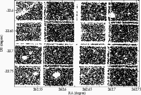
Figure 2: Position of all stars detected in field 5NP in J H and K_s with $\chi^{2}<1.5$ and $|sharp|<0.5$.

Given the complexity of the source distributions in our fields, a completeness estimation for number counts analyses would be unreliable. Indeed figure 2 illustrates the various instrumental, atmospheric and astrophysical effects on the number of stars detected. The gaps between the detectors are apparent due to our removal of the dithered image borders. The photometric conditions influence the overall completeness. Variations of the number counts between dither sets are due to changes in the atmospheric conditions and in particular in the seeing. Large holes are due to the presence of saturated stars. Variations of the number counts within chip images are also visible due to variations of the extinction. For example a dark cloud is clearly present in the top-left corner of figure 2.

3 Red Clump Giants as Distance Indicators: Deriving the distances

The main stellar populations observed in this survey are illustrated in figure 3, which is the colour-magnitude diagram (CMD) of the minor axis low-extinction standard field C32. In the blue part of the diagram lie foreground main-sequence disc stars. In field C32, since the extinction is low and because the central inner Galactic bulge clearly is spatially highly-concentrated with a small scale length, the bulge red giant branch (RGB) stars form a well-defined, almost single-distance RGB feature with a distinct red clump. The foreground disc red clump giants form a third sequence on the CMDs, roughly parallel to the disk main sequence stars, becoming fainter and redder as their distance and total extinction increase. The narrow intrinsic luminosity distribution of the red clump stars, apparent in this figure, illustrates their utility as good distance indicators.

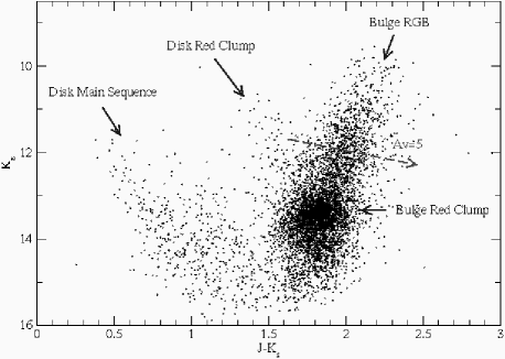
Figure 3: Colour-magnitude diagram of the bulge field C32 ($\ell=0\degr$, $b=1\degr$), using all stars detected in J,H and K_s with $\chi^{2}<1.5$ and $|sharp|<0.5$. The dotted arrow represents the movement of a star on this diagram due to an absorption of $A_{V}$=5 mag.

Given the high and variable extinction apparent in our fields, reddening independent magnitudes are a critical requirement. Such parameters can be derived using any two colours, given an extinction law, for example:

$${K_{s}}_{J-K_{s}}=K_{s}-{A_{K_{s}}\over A_{J}-A_{K_{s}}}(J-K_{s})$$ (1)

In the near-infrared, the extinction curve is well defined by a single power law function (e.g. Cardelli et al. 1989, Mathis 1990, He et al. 1995): $A_{\lambda}/A_{J}=(\lambda/\lambda_{J})^{-\alpha}$. As a consequence, and unlike optical studies such as Stanek et al. (1994), where extinction law variations remain a source of possible systematic uncertainty, our reddening independent magnitudes should not be significantly affected by variations of ISM properties along the different lines of sight, although estimates of $A_{V}$ would. In the following we adopt the coefficient $\alpha=1.73$ of He et al. (1995), leading to $A_{K_{s}}/E_{J-K_{s}}$ = 0.64, which agrees with the values reviewed by Mathis (1990).

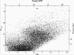
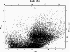
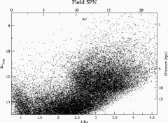
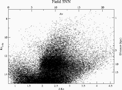
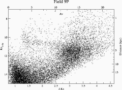
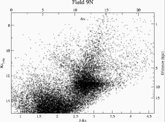
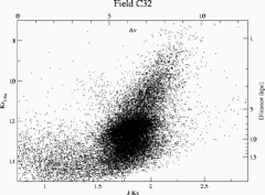
Figure 4: Colour magnitude diagrams using reddening independent magnitudes of all stars observed in J and K_s. In these figures, increasing extinction moves a star horizontally to the right, while increasing distance moves it vertically downwards. Locations of red clump stars on this diagram as a function of absorption and distance are given by the top and right hand axes.

In a colour magnitude diagram made with a reddening-independent magnitude, the effect of distance and extinction are disentangled: a star of a given spectral type moves vertically with distance, horizontally with extinction. Figure 4 illustrates, for each of our seven observed fields, how the location of a red clump star in the ($J-K_{s}$, ${K_{s}}_{J-K_{s}}$) diagram can be translated into an ($A_{V}$, distance) estimate. These diagrams therefore allow us to quantify the distribution of both stellar density and of the extinction along each line of sight. For example, in field 9P a clear flattening of the disc red clump distribution at ${K_{s}}_{J-K_{s}}\approx 10.5$ indicates the presence of a specific source of extinction located at about 3.5 kpc from the Sun, which increases $A_{V}$ by about 7.5 mag in only 1.5 kpc. This feature is consistent with the steep increase in absorption at 3.4-4 kpc seen at $\ell$=12.9° by Bertelli et al. (1995), that they associated with the molecular ring. In all our galactic plane fields, the bulk of bulge red clump stars become visible at $A_{V}\sim 10$ mag, and apparently suffer a range of internal extinction of more than $\Delta A_{V}\sim 5$ mag.

A clear difference between the red clump distance distributions is present between the different lines of sight, indicating that we have resolved the spatial structure of the inner Galaxy.

To quantify this, we determine the reddening-independent magnitude of the red clump, $m_{RC}$, by a non-linear least-squares fit of function 2 to the histogram of red giant stars (e.g. Stanek & Garnavich 1998, Salaris & Girardi 2002):

$$N(m)=a+bm+cm^{2}+{N_{RC}\over\sigma_{RC}\sqrt{2\pi}}\exp[-{(m_{RC}-m)^{2}\over 2\sigma_{RC}^{2}}]$$ (2)

The Gaussian term represents a fit to the bulge/bar red clump. The first three terms describe a fit to the background distribution of non-bulge-clump red giant stars, which in our case contains not only the other bulge giants, but also the disc red clump stars that fall into the bulge red clump. The foreground dwarf star sequence is eliminated on the CMDs by the criterion $K_{s}>4(J-K_{s})+b$, with b determined for each CMD to account for the different extinction. As distance and extinction grows, the mixing between faint dwarfs and giants increases. Only stars with ${K_{s}}_{J-K_{s}}<14$ mag will then be used, which corresponds to a limit in red clump star distance of about 15 kpc. These selection criteria ensure that all red clump stars at a distance of 9 kpc with photometric error smaller than 3 $\sigma$ and extinction smaller than $A_{V}$=15 are included in the analysis.

For given values of the red clump absolute magnitude and colour, a reddening independent magnitude provides a direct estimate of the distance modulus $\mu$ of red clump stars (equation 3), and so a direct measure of the line-of-sight variation in Galactic structure.

To check our calibration of the red clump colours, described below, and any effects of photometric incompleteness, we have estimated the distance modulus of the red clump from all three available reddening-independent magnitudes: ${K_{s}}_{J-K_{s}}$, $H_{H-K_{s}}$ and $J_{J-H}$:

$$\mu_{RC} = {K_{s}}_{J-K_{s}}+A_{K}/E_{J-K}(J-K_{s})_{0}-{M_{0}}_{K_{s}}$$ (3)

$$= H_{H-K_{s}}+A_{H}/E_{H-K}(H-K_{s})_{0}-{M_{0}}_{H}$$

$$= J_{J-H}+A_{J}/E_{J-H}(J-H)_{0}-{M_{0}}_{J}$$

These results are shown in figure 5.

We now require an upper limit to the reddening-independent magnitudes that can be analysed reliably in the fit to equation 2. For this, we derive a rough estimate of the relative completeness of each catalogue for each field ($J_{C}$,$H_{C}$,$K_{C}$) by determining when the number counts as a function of magnitude stop increasing. The different atmospheric, instrumental and astrophysical effects influencing this relative completeness have been described in section 2. The relative completeness of each reddening independent magnitude is then derived by combining these completeness estimates for each magnitude and field, using the mean colour of the giants ($(J-K)_{M}$) and adding a margin of 0.5 mag to take into account the spread in the mean colour:

$$max(K_{J-K}) = min(J_{C}-(J-K)_{M},K_{C})$$

$$-A_{K}/E_{J-K}*(J-K)_{M}+margin$$

The corresponding completeness-induced limits to our distance determinations down each line of sight are indicated for each passband and field in figure 5 by vertical lines. A maximum value of 16.1 is also apply due to the limit ${K_{s}}_{J-K_{s}}<14$ mag set before for the selection of giant stars.

The model fits to the spatial distribution of bulge/bar red clump stars down each line of sight are presented in figure 5. In general, the fits using the three different reddening independent magnitudes are all consistent within about 0.1 mag, expect for field 5NP where the dispersion is 0.2 mag. However no fit was possible using $J_{J-H}$ for fields 9P and 9N.

The exception is the two fields at positive longitude $\ell=5\degr$: no fit converged for any of the distance modulus estimators for fields 5PP and 5PN. The large spread in the red clump colour and magnitudes observed in those fields (figure 4) cannot be explained as an artefact of completeness nor by large photometric errors. The interpretation of these results is discussed further in the next section.

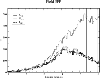
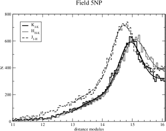
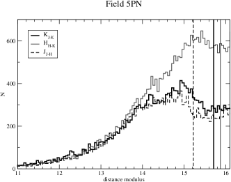
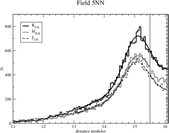
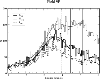
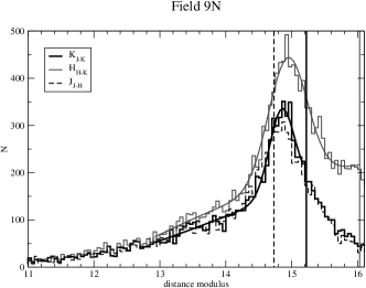
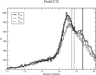
Figure 5: The distance modulus distributions down each line of sight, computed for red clump stars using reddening-independent magnitudes. The vertical lines show estimates of the photometric completeness limits. Fits to equation 2 are overlaid, where available.

In order to convert our reddening-independent magnitudes into true distance moduli, and hence into true spatial density distributions, we need to calibrate the near-IR intrinsic luminosity of the red clump stars. We used the true intrinsic colours of red clump stars predicted by the Padova isochrones in the 2MASS system (Bonatto et al. 2004) for a 10 Gyr old population of solar metallicity: ($J-K_{s}$)₀=0.68 and ($H-K_{s}$)₀=0.07. We then calibrate the absolute magnitude of the red clump ${M_{0}}_{K_{s}}$ using our data for field C32. The colour-magnitude diagram for field C32, shown in figure 3, is dominated by the bulge and located at 0° in longitude, its red clump stars should therefore be at the distance of the Galactic centre. If we assume the absolute red clump distance of $M_{K}=-1.61\pm 0.03$ mag, derived by Alves (2000) for the Hipparcos red clump, we obtain a distance for the Galactic center of $D_{GC}=7.6\pm 0.15$ kpc. Comparing the Padova isochrones provided in the Johnson-Cousins-Glass system by Girardi et al. (2002) and the 2MASS ones, we find that no correction need to be applied between the Alves (2000) K photometry and our K_s one for red clump stars. According to Salaris & Girardi (2002), a small population correction should be applied to the Alves (2000) calibration for bulge stars. Using their population correction for Baade’s window with solar metallicity we derive $M_{K}=-1.68$ mag and $D_{GC}=7.8$ kpc, while with enhanced $\alpha$-elements it leads to $M_{K}=-1.72$ mag and $D_{GC}=8.0$ kpc. However if we assume $\alpha$-enhancement, as we will see later on, we also have to change the assumed ($J-K_{s}$)₀, which leads us back to $D_{GC}=7.7\pm 0.15$ kpc. Those values are consistent with the latest Galactic centre distance estimates (e.g. Reid 1993, McNamara et al. 2000, Eisenhauer et al. 2003) which give $D_{GC}=8\pm 0.5$ kpc. Considering the different uncertainties in the absolute magnitude of the red clump, we decided to calibrate this latter to $M_{K_{s}}^{RC}=-1.72$ mag, assuming a distance for the Galactic centre of 8 kpc.

The results of our different fits to equation 2 have been averaged and are presented in table 2. The dispersion of the Gaussian fitted to equation 2, $\sigma_{RC}$, is the convolution of the true line of sight dispersion in distance of the red clump stars ($\sigma_{D}$), the intrinsic dispersion of the red clump luminosity ($\sigma_{0}$) and photometric errors ($\sigma_{e}$). Alves (2000) estimates $\sigma_{0}$ to be around 0.15-0.2 mag. The photometric errors are between 0.05 and 0.1 mag. An estimate of the dispersion due to the variation in distance modulus is then indicated in table 2, derived from the simple deconvolution $\sigma_{D}=\sqrt{\sigma_{RC}^{2}-\sigma_{0}^{2}-\sigma_{e}^{2}}$.

Table 2: This table presents both the mean and the line-of-sight dispersion in distances of bulge red clump stars for four different galactic longitudes. $\sigma_{m}$ is the Gaussian dispersion of the fits of equation 2 to the photometric data of figure 4, which are shown in figure 5. $\sigma_{D}$ is our estimate of the equivalent spread in distance, after deconvolution with the intrinsic red clump luminosity dispersion and photometric errors.

l	$\mu_{RC}$ (mag)	D (kpc)	$\sigma_{RC}$ (mag)	$\sigma_{D}$ (kpc)
-9.8°	14.90$\pm$0.04	9.5$\pm$0.2	0.25$\pm$0.03	0.6
-5.7°	14.97$\pm$0.04	9.9$\pm$0.2	0.40$\pm$0.01	1.5
0.0°	14.51$\pm$0.03	8	0.30$\pm$0.05	0.8
+9.6°	13.63$\pm$0.04	5.3$\pm$0.1	0.65$\pm$0.1	1.5

We studied the robustness of our results against different choices of isochrones. A different age changes the absolute magnitude of the red clump but not its colour, so as we fix $M_{K_{s}}^{RC}$ from our data the choice of age does not affect our results. However metallicity and enrichment in $\alpha$-elements does affect the colours. A change in [Fe/H] of 0.4 dex changes $J-K_{s}$ by about 0.08 mag, the higher the metallicity the redder the colour. Isochrones for $\alpha$-enhanced stars lead to $J-K_{s}$ bluer by about 0.1 mag. However as all is calibrated on field C32, the resulting distance estimates do not change by more than 0.3 kpc. However we note that the three different distance modulus estimates for field C32 (bottom of figure 5) agree much better with $\alpha$-enhanced isochrones (within 0.01 mag) than with the basic set (where the dispersion is 0.1 mag). On the other hand, for all the other fields the $\alpha$-enhanced isochrones lead to a larger dispersion. If we assume that we are not probing one but two different stellar populations, which would correspond to the bulge for field C32 and to a distinct Galactic bar for the other fields, such a difference would be expected. Chosing the $\alpha$-enhanced colors for the bulge field (McWilliam & Rich 1994, Matteucci et al. 1999) and the basic set for all the others would lead to an increase in distance modulus in all the ‘bar’ fields of about 0.1 mag. If we also consider an age difference, using an age of 6 Gyr (Cole & Weinberg 2002) for the bar fields would also add about 0.1 mag to the distance modulus. Figure 7 illustrates the effect of systematics in the assumed stellar populations: if we assume that the inner bulge is formed of an old population with enhanced $\alpha$ abundances, while the bar is formed of a younger population with solar abundances, the deduced distances show a much smaller dispersion from a galactic bar simple linear regression model. If confirmed by spectral observations, this implies a bar population which is formed from the inner disc, and not from the old bulge.

4 The structure of the inner Galaxy

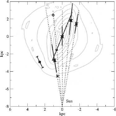
Figure 6: The Galactic plane seen from the north Galactic pole. Solid circles indicate the mean positions of the red clump giants determined in this analysis at Galactic longitudes of $\ell=\pm 9.7\degr$, $\ell=-5.7\degr$, and $\ell=0\degr$. Thick grey lines along the lines of sight through each mean distance represent the one$-\sigma$ range in distances deduced from a Gaussian fit to the red clump apparent distance modulus distribution, corrected for intrinsic red clump luminosity dispersion and photometric errors. The black line through the mean distances illustrates a Galactic bar of 3 kpc radius inclined at 22.5° to the Sun-Galactic Centre line. The background contour map is a plane projection of the Bissantz & Gerhard (2002) galactic bulge bar model, from their figure 11. The empty circles at $\ell=+5.7\degr$ are only indicative, as the more distant point may be confused by background disk stars, as discussed in the text. The small cross at 3.5kpc from the Sun along the direction $\ell=+9.7\degr$ indicates the position of a local high-extinction region detected in our photometry. The square to the left of the dotted lines through our data indicates the mean position of the red clump detected by Hammersley et al. (2000) at $\ell$=+27°.

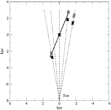
Figure 7: Same as figure 6, with the empty circles indicating the mean positions of the red clump giants determined with different isochrones for the bulge field at $\ell=0\degr$ and the other fields. The solid circles distances assume that the stellar population of all the fields are 10 Gyr old and of solar metallicity. The empty circles positions are computed assuming for the bulge field at $\ell=0\degr$ a 10 Gyr old population with enhanced $\alpha$-element abundances, while assuming for all the other fields a 6 Gyr old population of solar abundances.

Figure 6 summarises our derived spatial map of the inner Galaxy. As well as the mean distances down each line of sight, the range of distances corresponding to the deconvolved one-$\sigma$ dispersion in distance modulus is also illustrated. In spite of this representation, we emphasise that the true distribution in distance has no reason to be Gaussian, as it is linked to the geometry of the bar/bulge and to our viewing angle. Our observation angle biases both our distance and dispersion estimates, because of the larger volume, and hence probable larger number of stars present in the far side of our observation cone than in the near side. One should then keep in mind that our distance estimates will be slightly biased towards larger distances, especially for structures with a large true dispersion in distances, and as close to us as is observed at $\ell$=+9°.

Our mean red clump distances measured at $\ell=+9\degr$ and $\ell=-5\degr$ are consistent with the more recent bar models, particularly those derived considering both gas dynamics and available surface brightness luminosity distributions. Those models deduce a bar orientation with respect to the Sun -galactic centre direction of 15°$\la\phi_{bar}\la$ 35°(e.g. Gerhard 2001, Merrifield 2003). The model of Bissantz & Gerhard (2002) (their figure 11) is overlaid on figure 6. This model assumes a bar with an angle $\phi_{bar}=20$°, a length of 3.5 kpc and an axis ratio 10:3-4. The overall agreement with our direct distance determinations is rather good.

Our mean red clump distance derived at $\ell=-9\degr$ is however not simply consistent with the bar model described above. A single linear fit to all the four mean distances measured at $\ell=+9,0,-5,+9\degr$ has all four points more than 3$\sigma$ from the ‘best fit’. However the feature observed at $\ell=-9\degr$ does seem real: inspection of figure 4 shows a clear overdensity of the whole red giant branch at the same distance as the mean clump distance, determined to be $\sim$ 9 kpc, in this field. Moreover, in this line of sight, the most likely source of distance bias, the presence of disc red clump stars, would bias the distance estimate towards larger distances, not shorter. The red clump distance estimate at $\ell=-9\degr$ is consistent with that at $\ell=-5\degr$. A possible physical interpretation is that we have detected the signature of the end of the bar. Star count peaks have also been detected in this region in studies of old OH/IR stars by Sevenster (1999) and in the DENIS star counts by López-Corredoira et al. (2001). López-Corredoira et al. (2001) suggest that this local density maximum may be related to the red clump overdensity detected by Hammersley et al. (2000) at $\ell=27\degr$. The Hammersley et al. (2000) density maximum is indicated in figure 6 by a square.

The presence of these two local features at $\ell=27\degr$ and $\ell=-9\degr$ and their mean red clump distance estimates could imply the presence of a double triaxiality in the inner Galaxy, a double bar, or a triaxial bulge oriented at $\sim 22\degr$ with a longer, thiner bar oriented at $\sim 44\degr$. However, if such a second structure did exist, we should have detected its signature in our other survey fields. No such complex signature is evident (cf. figure 4). If two complex spatial distributions were projected down our lines of sight without being resolved, this would imply that our distance determinations are biased so that the angle of the first structure is in fact smaller than the 22° we measured, and that the spread of the red clump distances observed down each line of sight would encompass both structures. The latter does not seem to correspond to the rather small distance dispersions we derived, which are summarised in table 2. Furthermore, Picaud et al. (2003) do not detect a density excess at l=+21°, confirming that the structure seen at l=+27$\degr$ is probably local, and unrelated to the larger bulge or bar.

An alternative, and perhaps more consistent, interpretation of the $\ell=-9\degr$ structure we observe is the presence of a stellar ring or pseudo-ring at the end of the Galactic bar. If so, the bar and the stellar ring would have a radius of 2.3$\pm$0.25 kpc. Our observations at $\ell=+9\degr$ indicate that the radius of the bar is at least 2.7$\pm$0.2 kpc long. Those two determinations are consistent within one$-\sigma$. We note that assuming the bulge/bar stellar population differences used for figure 7 leads to a larger bar radius of about 3 kpc. A bar radius of about 2.5 kpc would agree with the model of Lépine & Leroy (2000) and Sevenster (1999), but is smaller than the value indicated by Gerhard (2001) in his review. The presence of a ring has been suspected by several authors. A molecular ring at about 4-5 kpc is a well known feature deduced from CO maps. Our detection of a step increase in the extinction distribution in field 9P (indicated by a cross in figure 6) could be associated with this molecular ring. Comeron & Torra (1996) link their derived distribution of ultracompact HII regions to the molecular ring, but also detect a star forming ring at about 2 kpc from the galactic centre. A stellar ring was suspected to lie at 3.5 kpc from the galactic centre by Bertelli et al. (1995). From an OH/IR star study Sevenster (1999) suggests that an inner ring lies between between 2.2 and 3.5 kpc. From star counts in the DENIS survey López-Corredoira et al. (2001) also argue for the presence of a stellar ring, mainly from the detection of a density peak at $\ell=-22\degr$ that, following Sevenster (1999), they associate with the tangential point to the 3-kpc arm, which is likely to be a (pseudo-)ring. The presence of a Galactic ring would also help to reproduce the observed microlensing optical depth (Sevenster & Kalnajs 2001).

Inner ring structures are indeed frequently observed in barred spirals. Most inner rings are in fact pseudo-rings, formed from the complex merging of inner bars and spiral structure (e.g. Buta & Combes 1996). Such a pseudo-ring structure is consistent with all the various detections of sub-structures between 2 and 4 kpc from the Galactic centre.

López-Corredoira et al. (2001) detect an asymmetry in the Galactic plane extinction distribution, with more extinction at negative than at positive longitudes. We do not confirm this result. The fact that we do not find any asymmetry in red clump giant extinction between positive and negative longitudes (figure 4), while there is an asymmetry in distance, is certainly consistent with a minimum in the dust distribution in this region. Interior of the bar outer radius a lower global density of stars and gas is often seen in observations of other galaxies. Several authors have suggested that such a stellar density decrease may be present in the Galactic disc (Binney et al. 1991, Bertelli et al. 1995, Freudenreich 1998, Lépine & Leroy 2000, López-Corredoira et al. 2004). Our observations are consistent with such a decrease in the dust distribution of the inner disc.

Another interesting feature often observed in barred galaxies is the presence of dust lanes associated with the bar. From DIRBE surface brightness maps, Calbet et al. (1996) suggested the presence of such a dust lane, preceding the Galactic bar. They estimate the extra absorption present at negative longitudes to be between 1 and 2.6 mag in K. The presence of such a feature is clearly ruled out by our observations.

4.1 The line of sight towards $\ell=+5\degr$

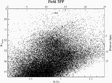
Figure 8: Colour - reddening independent magnitude diagram for field 5PP ($\ell=+5\degr$). This figure is derived from H&K_s photometry, which have the faintest completeness limits for this field.

The reddening-independent colour-magnitude diagram for the lines of sight towards $\ell=+5\degr$ (figure 8) differ significantly from those in other directions, in that the red clump stars indicate a very considerable range of distances, with no clear local maximum density. This is also very apparent in the relevant panels of figure 5, which show the corresponding distribution in distance modulus. The broad apparent distance distribution observed for the red clump stars at $\ell=+5\degr$ could be explained by the presence of two features, one at $\sim$ 6 kpc and a second at $\sim$ 11 kpc. Indeed, careful inspection of figure 8 suggests that the clump at ${K_{s}}_{H-K_{s}}\sim 12.5$ does not extend redder than H-K_s$>$1.2, while the fainter part, corresponding to distances greater than $\sim 10$kpc, extends beyond the photometric completeness limit. The first distance range is consistent with the bar structure confirmed above. It is also consistent with the fact that the OGLE data of Stanek et al. (1994), observed at a lower latitude of b=$-3.5\degr$, show similar photometric behaviour at $\ell=+5\degr$ compared to $\ell=-5\degr$, except for the expected shift in distance modulus.

The fainter feature in our low-latitude data could then be due to another structure, further away. This feature could be due to disc red clump stars. Indeed with increasing distance both the volume observed and the extinction increase, and considering the logarithmic relation between distance and magnitude, any distant red clump stars visible would concentrate in the high-extinction high distance-modulus bottom-right part of the CMD. Deeper data than we have available are then needed to determine if we are indeed seeing the distant disk beyond the bulge or a local structure which could be associated with the ring. This region is also interesting for further study as a broad velocity-width molecular clump has been detected at $5.2\degr<\ell<6.0\degr$ (e.g. Boyce & Cohen 1994, Bitran et al. 1997, Dame et al. 2001), which may be a manifestation of gas shocks (Kumar & Riffert 1997, Fux 1999). An estimate of the distance of those two structures, if the fainter one is real and indeed a local maximum, is presented in figure 6 as the open circles.

5 Conclusion

We have obtained, reduced and analysed deep wide-field near-infrared photometry of five lines of sight towards the Galactic bulge within 0.25° of the Galactic plane, using the CIRSI camera. This has provided a substantial improvement in our quantitative knowledge of inner Galactic structure, and in particular of the structure of the Galactic bar. Our use of near-infrared data allows us to determine reddening-independent magnitudes and to observe bulge red clump stars within the galactic plane, where the extinction is too high for optical studies. This allows the detection of tracer stellar populations independently of their scale height. Colour - reddening-independent magnitude diagrams have been shown to disentangle the effects of distance and extinction, allowing a direct conversion of red-clump star photometry ($J-K$,$K_{J-K}$) into an ($A_{V}$,distance) estimate. Those determinations have led to the following main results:

1. The presence of a triaxial structure at the centre of our Galaxy is confirmed. Its angle relative to the Sun-Galactic centre line is $\phi_{bar}=22\pm 5.5$°. It extends to at least 2.5 kpc from the Galactic Centre. A large axis ratio is excluded, but our data are consistent with a 10:3-4 ratio. In particular the distance dispersion of the bulge along the ($\ell=$0°,b=1°) line of sight is less than 1 kpc.

2. A structure present at $\ell=-9.8\degr$ is not aligned with this triaxiality. We suggest that the structure present at $\ell=-9.8\degr$ is likely to be the signature of the end of the Galactic bar, which is therefore circumscribed by an inner pseudo-ring.

3. A decrease in the dust distribution inside the bar radius is inferred from the extinction distribution in our fields.

4. Our observations are not consistent with the existence of the dust lane preceding the Galactic bar at negative longitudes suggested by Calbet et al. (1996).

References

- Alves (2000) Alves D. R., 2000, ApJ, 539, 732
- Beckett et al. (1997) Beckett M. G., Mackay C. D., McMahon R. G., Parry I. R., Piche F., Ellis R. S., 1997, in Proc. SPIE Vol. 2871, p. 1152-1159, Optical Telescopes of Today and Tomorrow, Arne L. Ardeberg; Ed. CIRSI: the Cambridge Infrared Survey Instrument. pp 1152–1159
- Bertelli et al. (1995) Bertelli G., Bressan A., Chiosi C., Ng Y. K., Ortolani S., 1995, A&A, 301, 381
- Bertin & Arnouts (1996) Bertin E., Arnouts S., 1996, A&A Suppl. Ser., 117, 393+
- Binney et al. (2000) Binney J., Bissantz N., Gerhard O., 2000, ApJ, 537, L99
- Binney et al. (1991) Binney J., Gerhard O. E., Stark A. A., Bally J., Uchida K. I., 1991, MNRAS, 252, 210
- Bissantz & Gerhard (2002) Bissantz N., Gerhard O., 2002, MNRAS, 330, 591
- Bitran et al. (1997) Bitran M., Alvarez H., Bronfman L., May J., Thaddeus P., 1997, A&AS, 125, 99
- Blitz & Spergel (1991) Blitz L., Spergel D. N., 1991, ApJ, 379, 631
- Bonatto et al. (2004) Bonatto C., Bica E., Girardi L., 2004, A&A, 415, 571
- Boyce & Cohen (1994) Boyce P. J., Cohen R. J., 1994, A&AS, 107, 563
- Buta & Combes (1996) Buta R., Combes F., 1996, Fundamentals of Cosmic Physics, 17, 95
- Calbet et al. (1996) Calbet X., Mahoney T., Hammersley P. L., Garzon F., Lopez-Corredoira M., 1996, ApJ, 457, L27+
- Cardelli et al. (1989) Cardelli J. A., Clayton G. C., Mathis J. S., 1989, ApJ, 345, 245
- Carpenter (2001) Carpenter J., 2001, AJ, 121, 2851+
- Cole & Weinberg (2002) Cole A. A., Weinberg M. D., 2002, ApJ, 574, L43
- Comeron & Torra (1996) Comeron F., Torra J., 1996, A&A, 314, 776
- Dame et al. (2001) Dame T. M., Hartmann D., Thaddeus P., 2001, ApJ, 547, 792
- de Vaucouleurs (1964) de Vaucouleurs G., 1964, in IAU Symp. 20: The Galaxy and the Magellanic Clouds Interpretation of velocity distribution of the inner regions of the Galaxy. pp 195–+
- Deguchi et al. (2000) Deguchi S., Fujii T., Izumiura H., Kameya O., Nakada Y., Nakashima J., 2000, ApJS, 130, 351
- Dwek et al. (1995) Dwek E., Arendt R. G., Hauser M. G., Kelsall T., Lisse C. M., Moseley S. H., Silverberg R. F., Sodroski T. J., Weiland J. L., 1995, ApJ, 445, 716
- Eisenhauer et al. (2003) Eisenhauer F., Schödel R., Genzel R., Ott T., Tecza M., Abuter R., Eckart A., Alexander T., 2003, ApJ, 597, L121
- Freudenreich (1998) Freudenreich H. T., 1998, ApJ, 492, 495
- Fux (1999) Fux R., 1999, A&A, 345, 787
- Gerhard (2001) Gerhard O. E., 2001, in ASP Conf. Ser. 230: Galaxy Disks and Disk Galaxies Structure and Mass Distribution of the Milky Way Bulge and Disk. pp 21–30
- Girardi et al. (2002) Girardi L., Bertelli G., Bressan A., Chiosi C. ., Groenewegen M. A. T., Marigo P., Salasnich B., Weiss A., 2002, A&A, 391, 195
- Häfner et al. (2000) Häfner R., Evans N. W., Dehnen W., Binney J., 2000, MNRAS, 314, 433
- Hammersley et al. (2000) Hammersley P. L., Garzón F., Mahoney T. J., López-Corredoira M., Torres M. A. P., 2000, MNRAS, 317, L45
- Hammersley et al. (1994) Hammersley P. L., Garzon F., Mahoney T., Calbet X., 1994, MNRAS, 269, 753
- He et al. (1995) He L., Whittet D. C. B., Kilkenny D., Spencer J ones J. H., 1995, ApJS, 101, 335
- Ibata & Gilmore (1995a) Ibata R. A., Gilmore G. F., 1995a, MNRAS, 275, 591
- Ibata & Gilmore (1995b) Ibata R. A., Gilmore G. F., 1995b, MNRAS, 275, 605
- Kuijken (1996) Kuijken K., 1996, in IAU Symp. 169: Unsolved Problems of the Milky Way Is There a Bulge Distinct from the Bar?. pp 71–+
- Kumar & Riffert (1997) Kumar P., Riffert H., 1997, MNRAS, 292, 871
- Lépine & Leroy (2000) Lépine J. R. D., Leroy P., 2000, MNRAS, 313, 263