VLT narrow-band photometry in the Lyman continuum of two galaxies at $z\sim 3$

We have performed narrow-band imaging observations with the Very Large Telescope, aimed at detecting the Lyman continuum (LC) flux escaping from galaxies at $z\sim 3$. We do not find any significant LC flux from our sample of two galaxies in the Hubble Deep Field South, at $z=3.170$ and $3.275$. The corresponding lower limits on the $F_{1400}/F_{900}$ flux density (per Hz) ratio are 15.6 and 10.2 (3-$\sigma$ confidence level). After correction for the intergalactic hydrogen absorption, the resulting limits on the relative escape fraction of the LC are compared with those obtained by different approaches, at similar or lower redshifts. One of our two objects has a relative escape fraction lower than the detection reported by Steidel et al. in a composite spectrum of $z\sim 3$ galaxies. A larger number of objects is required to reach a significant conclusion. Our comparison shows the potential of narrow-band imaging for obtaining the best limit on the relative escape fraction at $z\sim 3$. Stacking a significant number of galaxies observed through a narrow-band filter would provide constraint on the galactic contribution to the cosmic reionization.

1 Introduction

The observations of the finishing and the beginning reionization of intergalactic hydrogen at $z\sim 6$ and 20 (Becker et al., 2001; Kogut et al., 2003) combined with the later reionization of intergalactic He ii (Kriss et al., 2001; Zheng et al., 2004) at $z\sim 3$ are now placing constraints on the nature and the evolution of the ultra-violet (UV) background radiation. A dominant contribution of star-forming galaxies is suggested at $z>3$ before the density of luminous quasars become significant. This picture would gain additional support from direct measurements of the amount of Lyman continuum (LC) radiation released by galaxies into the intergalactic medium (IGM).

Direct measurements of the LC radiation from galaxies are, however, very challenging. In the local universe, they require space instruments sensitive at short UV wavelengths as well as galaxies slightly redshifted to avoid the neutral hydrogen opacity (continuum and line absorption) in the Galaxy. Observations of nearby star-forming galaxies with the Hopkins Ultraviolet Telescope (HUT) and the Far Ultraviolet Spectroscopic Explorer (FUSE) have led so far only to upper limits on the fraction of LC (or emitted 900 Å) photons that escape; the so-called escape fraction ($f_{\rm esc}$) is typically less than about 10% (Leitherer et al., 1995; Hurwitz et al., 1997; Deharveng et al., 2001). This is consistent with the values derived from the near-blackness of interstellar lines tracing the H i gas as observed with FUSE in five other starburst galaxies (Heckman et al., 2001).

At high redshifts, the increasing IGM opacity (absorption of the ionizing radiation by the neutral hydrogen), not to speak of galaxies becoming fainter, makes the observations difficult. Nevertheless, large ground-based telescopes can enter the competition at $z\ga 3$. Steidel et al. (2001) (hereafter S01) derived a 1500Å/900Å observed flux density ratio, $(F_{1500}/F_{900})_{\rm obs}=17.7\pm 3.8$ from a composite spectrum of 29 Lyman break galaxies (LBGs) at a mean redshift of 3.4 with Keck/LRIS. By comparison with models of the UV spectral energy distribution of star-forming galaxies, the flux density ratio, corrected for the IGM opacity, leads to the fraction of escaping LC (900Å) photons relative to the fraction of escaping non-ionizing UV (1500Å) photons. This is called the relative escape fraction ($f_{\rm esc,rel}$) and is different from the first definition of the escape fraction ($f_{\rm esc}$) used above for nearby galaxies. S01 interpreted their results as implying $f_{\rm esc,rel}\ga 50\%$.

However, not all $z\sim 3$ galaxies emit a significant LC radiation. Using the FORS2 spectrograph on the VLT, Giallongo et al. (2002) (hereafter G02) obtained 1-$\sigma$ lower limits on $(F_{1500}/F_{900})_{\rm obs}$ four times larger than the value of S01 for two bright LBGs. Heckman et al. (2001) also deduced a very low escape fraction for a gravitational lensed galaxies, MS 1512-cB58 at $z=2.7$ from the detailed analysis of interstellar absorption lines.

Observations have not been only spectroscopic. Imaging of galaxies at $z\sim 1$ with the FUV solar-blind detector of Space Telescope Imaging Spectrograph (STIS) have also provided constraints on the flux below the Lyman limit (Ferguson, 2001; Malkan et al., 2003). In particular, Malkan et al. (2003) (hereafter M03) have obtained lower limits of $(F_{1500}/F_{700})_{\rm obs}\ga 150$–1000 (1-$\sigma$), implying much lower LC escape fraction than in the galaxies of S01. Fernández-Soto et al. (2003) (hereafter FS03) have used the deep $U_{300}$ images of the Hubble Deep Field North (HDFN) and reported an average LC escape fraction of no more than 4% for 27 galaxies at redshifts $1.9<z<3.5$. As a number of galaxies in their sample have their $U_{300}$ fluxes contaminated by nonionizing UV photons, their analysis is based on models and indirect.

These conflicting results, as well as the difficulties of observations at high redshift, have led us to search for possibilities of improvement. We have first examined how the detection advantage of imaging over spectroscopy is actually working in the specific context of measuring faint LC radiation. On one hand, spectroscopy allows us to measure the LC flux close to the redshifted Lyman limit, where the average IGM opacity is not yet as large as it would be at shorter wavelength because of the Lyman valley (e.g., Møller & Jakobsen, 1990). On the other hand, broad-band measurements require a very large correction for the IGM opacity as we show in the current paper, because the effective wavelength becomes very short for objects selected at a redshift appropriate for avoiding contamination by nonionizing UV photons. The narrow-band imaging appears, therefore, as a natural compromise between the lower opacity offered by spectroscopy and the depth of detection offered by broad-band imaging.

We have, for the first time, attempted imaging observations from the ground, using the VLT, aimed at measuring the LC radiation from galaxies at high redshifts through a narrow-band filter. The goal of this paper is twofold: (i) reporting the data and their interpretation in terms of the relative escape fraction, and (ii) validating the narrow-band photometric approach by quantitative comparisons.

In Sect. 2, we describe the details of our strategy, the choice of the filter, the target selection based on photometric redshifts, the spectroscopic observations for confirming redshifts and the imaging observations. Data reduction and results are described in Sect. 3. Their interpretation in terms of relative escape fraction are presented in Sect. 4. A comparison of the constraints reached with those from other observations is given in Sect. 5, where we also discuss the absolute escape fraction. The final section is devoted to our conclusions.

We adopt a flat $\Lambda$-dominated cosmology with $\Omega_{\Lambda}=0.7$ and $\Omega_{\rm m}=0.3$, and the current Hubble constant $H_{0}=70$ km s^-1 Mpc^-1 to estimate luminosities.

2 Observations

2.1 Filter selection

A direct and unambiguous detection (or upper limit) of the LC escaping from galaxies requires a lower redshift limit of the target galaxies to push out all emission red-ward of the Lyman limit beyond the long wavelength cut-off of the filter transmission. The cut-off wavelength is defined practically at 1% transmission relative to the peak. Since the IGM opacity rapidly increases with the source redshift (e.g., see Fig. A.2), the limiting redshift should be set as low as possible. The $OII+44$ narrow-band filter, whose long wavelength cut-off is the smallest among all filters of FORS on VLT, was selected for our observation. Accordingly, galaxies with $z\geq 3.18$ must be selected. We note here that the long wavelength cut-off of this filter is smaller than that of the $U_{300}$ of WFPC2 on the HST as shown in Fig. 1. Indeed, the redshift limit for the $U_{300}$ would be $z\geq 3.33$.

Figure 1: Transmission curves of the FORS $OII+44$ filter (solid) and the HST $U_{300}$ (dashed).

2.2 Observed field and target galaxies

As the redshift surveys in the southern celestial sphere had not produced a large number of galaxies with spectroscopic redshift ($z_{\rm sp}$) larger than 2, we had to select galaxies based on photometric redshift ($z_{\rm ph}$) in the first phase of our observations. Labbé et al. (2003) made a catalog of photometric redshift of galaxies in the Hubble Deep Field South (HDFS; Williams et al. 2000) by using their ultra-deep near-infrared images obtained with VLT/ISAAC and HST/WFPC2 optical images. Thus, we selected the HDFS/WFPC2 field as our target field.

There are 24 galaxies with $I_{814}\leq 25.0$ mag(AB) and $z_{\rm ph}\geq 2.5$ in the field. We set this lower limit of $z_{\rm ph}$, taking into account the 2-$\sigma$ uncertainty of $z_{\rm ph}$ for $z\sim 3$ ($\sigma\approx 0.08(1+z)$ noted in Labbé et al. 2003). Eight of them have $z_{\rm ph}$ larger than 3.18. On the other hand, six out of 24 have $z_{\rm sp}$, but all of them are less than 3.18. We note that all the known $z_{\rm sp}$ are smaller than the corresponding $z_{\rm ph}$.

An accurate redshift is essential to avoid contamination from nonionizing photons. We need a redshift accuracy of the order of 0.01. Since the accuracy of $z_{\rm ph}$ is not sufficient, we performed spectroscopic observations with FORS2 on VLT using the MXU mode. A full description of the observation will be published elsewhere (Iwata et al. in preparation). Here, we summarize the results briefly.

Because of the limitation of the slit-let configuration, we were able to take spectra of only 15 galaxies out of the above 24 galaxies. Five out of the 15 galaxies have known $z_{\rm sp}$ and 7 of them have $z_{\rm ph}>3.18$. The choice of galaxies was made with a priority given to more luminous galaxies and galaxies with $z_{\rm ph}>3.18$. Additionally, we took spectra of galaxies with $z_{\rm ph}\geq 2.5$ but $I_{814}>25.0$ mag(AB), for which we could configure the slit-let. Among these galaxies, one has $z_{\rm sp}$ previously measured. We ended up with obtaining 13 $z_{\rm sp}$: seven of them are new measurements and the remaining six are confirmations of the previous results.

Among the new redshifts, we got only one galaxy with a high enough redshift, $z_{\rm sp}=3.275$ (HDFS 1825), in contrast to the expectation from photometric redshifts. Indeed, for the 13 galaxies with $z_{\rm sp}$, we always find $z_{\rm sp}<z_{\rm ph}$, again. There is another galaxy with $z_{\rm sp}=3.170$ (HDFS 85) which was confirmed by our spectroscopy. This redshift is slightly smaller than the limiting redshift, however, the transmission efficiency of the $OII+44$ filter at the Lyman limit of the galaxy is as small as a few percent of the peak efficiency (see Fig. 1). The contamination of nonionizing photons is small enough, especially in the context of upper limit measurements. Therefore, our final sample consists of the two galaxies. We have no other explanations for this small number of target galaxies than a systematic error in the estimation of $z_{\rm ph}$.

2.3 Imaging observations

The HDFS field was observed through the $OII+44$ narrow-band filter with FORS1 and the TK2048EB4-1 detector chip in service mode from 29 June 2003 to 28 August 2003. The standard resolution collimator was adopted, giving a pixel scale of $0.^{\prime\prime}2$ per pixel. The field of view is $6.^{\prime}8\times 6.^{\prime}8$ and covers the whole area of the HDFS/WFPC2 field. Each image was taken with a small dithering (typically $10^{\prime\prime}$) and a typical exposure time of 1,080 sec. The seeing size of each image was $0.^{\prime\prime}39$–$1.^{\prime\prime}23$, typically $\sim 0.^{\prime\prime}8$. We secured 38 images of the field. The effective exposure time is 40,636 sec (i.e. about 11h). Table 1 shows a summary of the observations.

Table 1: Details of the imaging observations.

Dates (year 2003)	June 29, 30; July 5, 28; August 1, 28
Instrument	FORS1 on VLT
Collimator	standard resolution
CCD	$2048\times 2046$ pixels
Pixel scale	$0.^{\prime\prime}2$/pixel
Field of view	$6.^{\prime}8\times 6.^{\prime}8$
Filter	$OII+44$
Central wavelength	371.7 nm
Transmission FWHM	7.3 nm
Seeing	$\sim 0.^{\prime\prime}8$
Effective exposure time	40,636 sec

3 Data reduction and results

3.1 Final image

Figure 2: Close-up of sample galaxies through the $OII+44$ filter (VLT/FORS, this work), and the $I_{814}$ filter (HST/WFPC2, Williams et al., 2000). The FOVs are $20^{\prime\prime}\times 20^{\prime\prime}$. For the object 85, the image center is $6^{\prime\prime}$ shifted from the object position, because it is close to an edge of $I_{814}$ image.

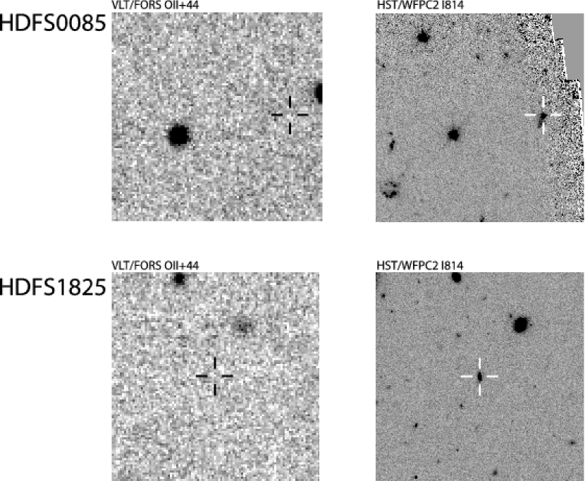
The image data reduction was carried out in a standard manner, using IRAF. The bias subtraction was made using over-scanned regions. Normalized twilight sky frames in each observing night were used for flat fielding. We selected 25 stars in the field and used them to register the 38 frames. After registration, the rms of residual shifts was 0.03 pixel. These stars were also used for an airmass correction. We found a slope of magnitude dependence on airmass of $-0.45$, and we corrected observed counts as it would have been observed at the zenith. The stability of the observing conditions is confirmed by measuring the corrected counts of these stars; the rms errors in counts are less than 0.05 mag for 19 stars brighter than 22 mag(AB) through the $OII+44$ filter among the above 25 stars. Then, the IRAF task IMCOMBINE was used to sum the frames. We took averages of each pixel adopting a 3-$\sigma$ clipping. FWHM of stellar objects in the final image is $\sim 1^{\prime\prime}$. Fig. 2 shows the close-up images of the two sample galaxies through the $OII+44$ filter and through the $I_{814}$ filter of HST/WFPC2. Neither galaxy seems to be seen through the $OII+44$ filter.

3.2 Photometry

Three standard stars, Feige 110, G 93-48, and LTT 9491, were also observed through the same filter. These frames were processed in the same way as the HDFS frames. The absolute AB magnitude of these stars were calculated from the spectral table provided on ESO web page. We found that the airmass dependence for the standard stars was $-0.58$ which is somewhat larger than that from stars in the HDFS frames. We derived the photometric zero point for the $OII+44$ filter at the zenith as 22.98 from the airmass slope of the standard stars. The zero point changes less than 0.02 mag if we adopt the airmass slope $-0.45$ which we used for correction of the HDFS frames.

To reduce background fluctuations, we apply a Gaussian smoothing to the final image adapted to the expected size of the sample galaxies through the $OII+44$ filter. The size through the HST/WFPC2 $B_{450}$ filter is a reasonable approximation because the central wavelength is close to that of the $OII+44$ filter and we are seeing the light from massive stars in both filters. Diameters of $0.^{\prime\prime}72$ (HDFS 85) and $0.^{\prime\prime}41$ (HDFS 1825) are estimated from the half-light radii of the galaxies through the $B_{450}$ filter reported in the HDFS WFPC2 catalog version 2 (Casertano et al., 2000). We adopt $2.5\times 2.5$ pix as the smoothing scale. The FWHM of the PSF in the smoothed image is 8.33 pixel ($=1.^{\prime\prime}7$).

None of the sample galaxies was detected at a 3-$\sigma$ level in the smoothed $OII+44$ image. The upper limit on their flux density has been based on the smoothed PSF size because they are smaller than the PSF. The measured rms fluctuations within a square box of $1.^{\prime\prime}7\times 1.^{\prime\prime}7$ in the smoothed image around the sample galaxies translate into 3-$\sigma$ limiting magnitudes of 27.37 mag(AB) and 27.40 mag(AB) for HDFS 85 and 1825, respectively.

In Table 2, we summarize the photometric measurements of the two sample galaxies. Photometric data with HST are taken from the HDFS WFPC2 catalog version 2 (Casertano et al., 2000). In this table, all upper limits are 3-$\sigma$ level. Our limiting magnitude is comparable with that of the HDFS in the $U_{300}$ for the size of our sample galaxies, although the HDFS limiting magnitude for point source is deeper than ours (Casertano et al., 2000).

Table 2: Photometric properties of sample galaxies.

ID	85	1825
$\alpha$ (J2000)	22 32 46.91	22 32 52.03
$\delta$ (J2000)	$-$60 31 46.9	$-$60 33 42.6
redshift	3.170	3.275
$OII+44$ (nJy)	$<44.88$	$<39.81$
${U_{300}}^{b}$ (nJy)	$<101.8$	$<42.09$
$B_{450}$ (nJy)	$392.08\pm 12.02$	$181.98\pm 6.51$
${V_{606}}^{c}$ (nJy)	$698.68\pm 8.86$	$404.91\pm 4.26$
${I_{814}}^{c}$ (nJy)	$859.63\pm 17.82$	$504.49\pm 7.58$

4 Lyman continuum escape fraction

From the upper limits obtained above on the LC flux of the two galaxies at $z=3.170$ and $z=3.275$, we try here to estimate the escape fraction of LC photons. As mentioned in the introduction, the term of escape fraction has been used in at least two ways. We first clarify the definition of the escape fractions.

4.1 Definition of escape fractions

We define two escape fractions. One is

$$f_{\rm esc}\equiv\frac{L_{\rm LC}^{\rm out}}{L_{\rm LC}^{\rm int}}=\exp(-\tau_{\rm LC}^{\rm ISM})\,,$$ (1)

where $L_{\rm LC}^{\rm int}$ is the intrinsic LC luminosity density (per Hz) of a galaxy, $L_{\rm LC}^{\rm out}$ is the LC luminosity density just outside of the galaxy (not the observed one, see below), and $\tau_{\rm LC}^{\rm ISM}$ is the opacity of the interstellar medium (ISM) for LC photons in the galaxy. The other is

$$f_{\rm esc,rel}\equiv f_{\rm esc}\left(\frac{L_{\rm UV}^{\rm out}}{L_{\rm UV}^{\rm int}}\right)^{-1}=f_{\rm esc}\exp(\tau_{\rm UV}^{\rm ISM})\,,$$ (2)

where $L_{\rm UV}^{\rm int}$, $L_{\rm UV}^{\rm out}$, and $\tau_{\rm UV}^{\rm ISM}$ are the intrinsic luminosity density, outside luminosity density, and the ISM opacity of the nonionizing UV photons, respectively. Hereafter, the former is called the absolute escape fraction, and the latter is called the relative escape fraction.

The IGM opacity should be taken into account for photons with a wavelength shorter than the Ly$\alpha$ line at the source rest-frame. Namely, the observed luminosity density becomes $L_{\lambda}^{\rm obs}=L_{\lambda}^{\rm out}\exp(-\tau_{\lambda}^{\rm IGM})$ for the rest-frame wavelength $\lambda<1216$ Å, and $L_{\lambda}^{\rm obs}=L_{\lambda}^{\rm out}$ otherwise if the IGM dust extinction is negligible. Indeed, based on observations of distant supernovae and on the thermal history of the IGM, Inoue & Kamaya (2004) have recently shown that the IGM dust extinction against $z\sim 3$ sources should be less than 1 mag in the observer’s $B$-band. Taking a wavelength longer than the Ly$\alpha$ line for the UV wavelength (e.g., $\sim 1500$ Å), we have

$$f_{\rm esc,rel}=\frac{(L_{\rm UV}/L_{\rm LC})_{\rm int}}{(F_{\rm UV}/F_{\rm LC})_{\rm obs}}\exp(\tau_{\rm LC}^{\rm IGM})\,,$$ (3)

where we have replaced the observed luminosity density ratio into the observed flux density ratio. Hence, the relative escape fraction can be estimated from the observed UV-to-LC flux density ratio if we know the intrinsic UV-to-LC luminosity density ratio and the IGM opacity. Moreover, the absolute escape fraction can be estimated from the relative escape fraction via equation (2) if we know the ISM opacity for nonionizing UV photons.

4.2 Intrinsic luminosity density ratios

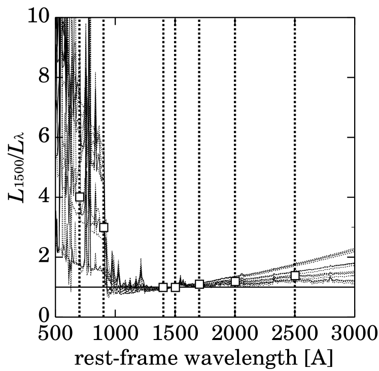
The intrinsic UV-to-LC luminosity density ratio is still very uncertain observationally. As noted by S01, we must rely exclusively on models. Here we adopt the Starburst 99 model (Leitherer et al., 1999). From this model, we obtain $(L_{1500}/L_{900})_{\rm int}=1.5$–5.5 as shown in Fig. 3, assuming a constant star formation rate, the Salpeter initial mass function with the mass range of 0.1–100 $M_{\odot}$, and the metallicity of 0.001–0.02 (the solar value is 0.02). The luminosity density ratios mainly depend on the duration since the onset of star formation; the ratio starts from a small value, monotonically increases with time, and saturates at a larger value after several $10^{8}$ yrs. In this paper, we adopt $(L_{1500}/L_{900})_{\rm int}=3.0$ according to the value adopted by S01.

Since the UV and LC wavelengths actually depend on the filter adopted and the source redshift, we have to adjust the intrinsic UV-to-LC luminosity density ratios to the correct wavelengths. Some of the ratios, relative to 1500 Å, are displayed in Fig. 3 as open squares and summarized in Table 3. This table will be used to calculate the UV-to-LC luminosity density ratio appropriate for each individual galaxy in Sects. 4.4 and 5.1. As illustrated in Fig. 3, the uncertainties on the luminosity density ratios are 20–50%.

Table 3: Adopted intrinsic ratios of luminosity densities relative to 1500 Å.

$x$	$(L_{1500}/L_{x})_{\rm int}$
(Å)
700	4.0
900	3.0
1400	1.0
1700	1.1
2000	1.2
2500	1.4

Figure 3: Intrinsic ratio of luminosity density at 1500 Å to that at the wavelength along horizontal axis. Thin dotted curves show 16 cases of the combination of 4 metallicities (0.001, 0.004, 0.008, and 0.02) and 4 ages (0 yr, 10 Myr, 100 Myr, and 1 Gyr), assuming a constant star formation and the Salpeter initial mass function with 0.1–100 $M_{\odot}$. Open squares are fiducial ratios adopted in the text at 7 wavelengths marked by thick dotted vertical lines. Unit of luminosity densities is erg s^-1 Hz^-1.

4.3 IGM opacity

An average opacity of the IGM can be estimated from the number distribution functions of the Lyman $\alpha$ forest and denser H i absorbing clouds (e.g., Madau, 1995). The number of H i clouds per unit interval of neutral hydrogen column density $N_{\rm HI}$ and per unit redshift $z$ interval can be expressed as $\partial^{2}{\cal N}/\partial z\partial N_{\rm HI}\propto(1+z)^{\gamma}N_{\rm HI}^{-\beta}$. Kim et al. (2002) have shown that the observed Lyman $\alpha$ forest data can be fitted with $\beta=1.5$, and $\gamma=2.5$ for $z\geq 1.1$ and $\gamma=0.2$ for $z<1.1$, by combining their high-$z$ data with the low-$z$ data of Weymann et al. (1998).

In contrast to previous approaches (e.g., Madau, 1995), we have shown in Appendix that not only the column density distribution but also the number evolution of the denser clouds (essentially, Lyman limit systems) can be reasonably described by the same function as that obtained for the Lyman $\alpha$ forest by Kim et al. (2002). Based on this distribution function, we calculate an average IGM opacity, $\langle\tau^{\rm IGM}_{\lambda_{\rm obs}}(z_{\rm S})\rangle$, for a source with a redshift, $z_{\rm S}$, at an observed wavelength, $\lambda_{\rm obs}$ by an analytic approximation formula presented in Appendix as equations (A.4–6). As seen in Appendix, our opacity is quantitatively very consistent with the value measured and adopted by S01, and shows a reasonable agreement with the opacity model of Bershady et al. (1999). Finally, we integrate the IGM opacity over the filter transmission when we make a correction for the IGM absorption in order to derive the escape fraction from the photometric data. In the integration, we always assume a flat spectrum because we do not know the spectral shape of LC exactly.

4.4 Estimation of relative escape fraction

By combining the upper limit of the flux density through the $OII+44$ filter with the measurement of the flux density through the HST’s $V_{606}$, whose wavelength corresponds to the rest-frame $\sim 1400$ Å for our sample, we obtain a lower limit on the observed ratio $(F_{1400}/F_{900})_{\rm obs}$. This ratio has to be corrected for the Galactic extinction before estimating the relative escape fraction. For HDFS field, $E(B-V)=0.028$ mag (Schlegel, et al., 1998), which corresponds to the Galactic extinction of $A_{V_{606}}-A_{OII}=-0.050$ mag if we adopt the standard extinction law of our Galaxy (e.g., Whittet, 2003). Therefore, we obtain the 3-$\sigma$ lower limits of the corrected flux density ratio $F_{1400}/F_{900}$ of 15.57 and 10.17 for HDFS 85 ($z=3.16$) and HDFS 1825 ($z=3.27$), respectively.

Assuming $(L_{1400}/L_{900})_{\rm int}=3.0$ as found from Table 3 and mean IGM opacities integrated over the filter transmission, we obtain 3-$\sigma$ upper limits on the relative escape fraction as 72% and 216% for HDFS 85 and 1825, respectively. As found in equation (2), the relative escape fraction is not restricted to less than 100%, because it is the escape fraction relative to that of nonionizing UV photons. The obtained values are summarized in the top 2 lines of Table 4.

Since uncertain assumptions on the ISM dust extinction are inevitable for the calculation, the estimation of the absolute escape fraction is left for the following section (§5.2), where we will discuss these issues in detail.

Table 4: Summary of related observations and escape fractions.

Redshift range/method/	redshift	$(F_{\rm UV}/F_{\rm LC})_{\rm obs}$	$\tau_{\rm LC}^{\rm IGM}$	${f_{\rm esc,rel}}^{a}$	$\lambda_{\rm UV},\lambda_{\rm LC}$	$L_{\rm UV}$	$A_{\rm UV}$	ref.	${f_{\rm esc}}^{a}$
galaxy name				(%)		($10^{29}$ erg s-1 Hz-1)	(mag)		(%)
(1)	(2)	(3)	(4)	(5)	(6)	(7)	(8)	(9)	(10)
$z\sim 3$
Narrow-band photometry (this work)
HDFS 85	3.170	$>15.57$	1.32	$<72$	1	1.59	1.6	1	$<17$
HDFS 1825	3.275	$>10.17$	1.99	$<216$	1	0.970	1.9	1	$<38$
Spectroscopy
composite (29 galaxies)	3.40	$17.7\pm 3.8$	1.50	$76\pm 16$	2	1.60	0.26	…	$60\pm 13$
DSF 2237+116 C2	3.319	$>24$	1.41	$<51$	2	3.15	3.8	2	$<1.5$
Q0000-263 D6	2.961	$>23$	1.04	$<37$	2	4.85	2.3	2	$<4.5$
Broadband photometry
FLY99: 957	3.367	$>2.34$	4.63	…	3	0.116	…	…	…
FLY99: 825	3.369	$>11.9$	4.64	…	3	0.617	…	…	…
FLY99: 824	3.430	$>7.89$	4.94	…	3	0.638	…	…	…
$z\sim 1$
Broadband photometry
Cl J0023+0423:[LPO98a]022	1.1074	$>187$	0.53	$<3.0$	5	0.967	1.3	3	$<0.91$
CFRS 03.1140	1.1818	$>308$	0.59	$<1.7$	6	2.56	…	…	$<1.7$
CFRS 10.1887	1.2370	$>119$	0.63	$<4.5$	6	0.969	…	…	$<4.5$
CFRS 10.0239	1.2919	$>228$	0.68	$<2.5$	6	2.28	…	…	$<2.5$
CFRS 10.1168	1.1592	$>163$	0.57	$<3.1$	6	0.802	…	…	$<3.1$
LDSS2 10.288	1.108	$>102$	0.53	$<5.5$	5	0.859	…	…	$<5.5$
HDF:iw4 1002 1353	1.221	$>67.8$	0.62	$<10.0$	4	0.513	2.6	4	$<0.91$
CFRS 14.0547	1.160	$>348$	0.57	$<1.8$	4	1.55	2.2	4	$<0.24$
CFRS 14.0154	1.1583	$>192$	0.57	$<3.4$	4	0.610	2.9	4	$<0.24$
SSA 22-16	1.36	$>165$	0.74	$<4.6$	4	1.05	0.20	4	$<3.8$
CFRS 22.1153	1.3118	$>125$	0.54	$<5.0$	4	1.00	1.6	4	$<1.1$
Nearby galaxies
Spectroscopy
Mrk 54	0.0448	$>111$	…	$<2.7$	2	0.83	0.92	5	$<1.2$
Mrk 496	0.0293	$>7.5$	…	$<40$	2	0.13	2.4	6	$<4.4$
Mrk 66	0.0218	$>7.6$	…	$<39$	2	0.064	1.2	6	$<13$
Mrk 1267	0.0193	$>7.8$	…	$<38$	2	0.068	3.5	6	$<1.5$
IRAS 08339+6517	0.0187	$>12$	…	$<25$	2	0.34	1.6	6	$<5.7$

5 Discussions

5.1 Comparison with other observations of Lyman continuum

In the following section, we compare the limits obtained in Sect. 4.4 for our two galaxies with those already presented in the literature (see Sect. 1). To do this, we have compiled all the UV-to-LC flux density ratios published in refereed journals. The data are summarized in Table 4, where they are divided into several categories depending on the source redshift and the observational technique. For the broad-band $U_{300}$ data, we restrict ourselves to the galaxies with $z_{\rm sp}>3.33$ in order to avoid any contamination of nonionizing UV photons. Thus, we took three galaxies from the list of FS03.

We first compare the observed UV-to-LC flux density ratio ($F_{\rm UV}/F_{\rm LC}$, column 3 in Table 4) and the estimated relative escape fraction ($f_{\rm esc,rel}$, column 5), using the intrinsic luminosity density ratios (Sect. 4.2) and the IGM opacity model (Sect. 4.3, column 5), which are tailored to the specific wavelength and the filter bandpass (column 6) for each individual galaxy.

5.1.1 $z\sim 3$ galaxies

The column 3 in the top of Table 4 shows that our two observed lower limits of $F_{\rm UV}/F_{\rm LC}$ are comparable to those already obtained for galaxies at $z\sim 3$. G02 have reached constraints about two times better than ours, because their two objects are more than two times intrinsically brighter. Our objects, as those of S01, are comparable in luminosity to the $L_{*}$ of $z\sim 3$ LBGs (see column 7; $L_{*}(z=3)\sim 1\times 10^{29}$ erg s^-1 Hz^-1; Steidel et al., 1999; Adelberger & Steidel, 2000).

In terms of relative escape fraction (column 5), we add one more object (HDFS 85) to the two galaxies of G02 that have been reported with a relative escape fraction lower than the detection of S01. Because of the small sample size, these lower limits remain consistent with the relative escape fraction of S01. Although we have applied a mean IGM opacity for simplicity, a line of sight with larger than average opacity cannot be ruled out for an individual galaxy (not to speak of an unusual object as the escape is probably a random phenomenon).

The broad-band $U_{300}$ photometry in the HDFN reaches similar lower limits on $F_{\rm UV}/F_{\rm LC}$ (it would have reached slightly better values at the same luminosity level as ours). This, however, does not result in interesting constraints on the relative escape fraction because of the IGM opacity. The IGM opacity through the $U_{300}$ filter, with an effective wavelength of 700 Å in the source rest-frame, is much larger than those at wavelengths closer to the rest 900 Å (column 4). Since meaningful constraints on the relative escape fraction are not reached, this sample will be removed from discussions in terms of the absolute escape fraction presented below.

The top of Table 4 is also interesting for a comparison of methods of observations and a validation of future approaches. As expected, the narrow-band photometry can provide better constraints than spectroscopy. The better constraints of G02 are actually due to the high luminosity of the objects. If our sample had a similar luminosity to the galaxies of G02, say, $L=4\times 10^{29}$ erg s^-1 Hz^-1, we would have obtained $F_{\rm UV}/F_{\rm LC}\ga 40$ (3-$\sigma$ level). The broad-band photometry is disqualified by the IGM opacity contribution (or requires the help of models that lead to less direct constraints). The narrow-band photometry can provide, even for a single $L_{*}$ LBG, a lower limit on $F_{\rm UV}/F_{\rm LC}$ comparable with that measured in the composite spectrum of 29 galaxies by S01. Stacking a significant number of galaxies observed through a narrow-band filter will be able to go much deeper. We can also average the IGM opacity against any unusual line of sight in the stacking process. Such an approach would allow a significant comparison with the result of S01 and reveal which fraction of high-$z$ galaxies have high relative LC escape fraction.

5.1.2 $z\sim 1$ galaxies

Thanks to the high sensitivity of the HST/STIS, M03 have obtained very good lower limits on the flux density ratio of 11 galaxies at $z\sim 1$, $F_{\rm UV}/F_{\rm LC}>70$–350 at 3-$\sigma$ confidence level (column 3 in the middle of Table 4). With the correction for the average IGM opacity described in section 4.3, these ratios are converted to upper limits on the relative escape fraction of 2–10% (column 5). The luminosities of this sample are similar to $L_{*}$ of $z\sim 3$ LBGs (column 7).

The average IGM opacity (column 4) is much smaller than those at high redshift, but not completely negligible as assumed by M03, if we consider the Lyman limit systems (LLSs) which dominate the IGM opacity for $z\sim 1$ galaxies. The rarity of LLSs favors a statistical treatment rather than the average opacity adopted above. Based on the number distribution function of the IGM clouds assumed here (see Appendix), the expected number of LLSs within the wavelength range observed by M03 (1300 Å $\la\lambda_{\rm obs}\la$ 1900 Å) is about 0.3. Roughly speaking, for one-third of the objects of M03, the LLSs would loosen the constraints obtained under the assumption of no IGM opacity. In this sense, the number of galaxies in M03 is large enough to conclude a very small relative escape fraction for their objects.

5.1.3 Nearby galaxies

Although the upper limits on the LC from nearby galaxies have been estimated from their H$\alpha$ fluxes directly in terms of absolute escape fraction (Leitherer et al., 1995; Hurwitz et al., 1997; Deharveng et al., 2001), it is possible to evaluate the observed lower limits of $F_{\rm UV}/F_{\rm LC}$ for comparison with higher $z$ objects (the bottom part of Table 4; Table 1 in Deharveng et al., 2001). Except for Mrk 54, these limits, corrected for the foreground absorption by the Galactic HI and H₂ gas, are not better than those obtained at high-$z$ (column 3). The low luminosity of the sample galaxies is one of the causes (column 7). Nevertheless, moderate upper limits are obtained for the relative escape fraction, $<25$–40% (3-$\sigma$ confidence level; column 5), because no correction for the IGM opacity is necessary. For Mrk 54, whose luminosity is similar to those of our sample (column 7), the observed lower limit of Deharveng et al. (2001) translates into an upper limit on the relative escape fraction of 3% comparable to those for $z\sim 1$ galaxies of M03 (column 5).

5.2 Absolute escape fraction

As discussed above and shown by equation (2), estimating the absolute escape fraction from the relative escape fraction requires an evaluation of the dust attenuation within each galaxy which is often difficult and uncertain (e.g., Buat et al., 2002; Pettini et al., 1998; Meurer et al., 1999). Although the infrared to UV flux ratio is a good estimator of the UV attenuation (Buat et al., 1999; Gordon et al., 2000), the infrared fluxes for high-$z$ galaxies are not available yet. Here, we adopt a calibration between the nonionizing UV slope and the UV attenuation proposed by Meurer et al. (1999) for simplicity. However, we should keep in mind that the calibration depends on the type of galaxies, starburst or not (Bell, 2002; Kong et al., 2004).

The UV slope of the galaxies listed in Table 4 have been searched in the literature, or, if not available, estimated from broad-band measurements with the assumption of a power-low spectrum ($f_{\lambda}\propto\lambda^{\beta}$) (references in column 9 of Table 4). This was not possible for some galaxies of M03 because their colors in the rest-frame $\lambda<3000$ Å are not available. For the composite spectrum of S01, we estimated the UV attenuation from the reported mean $E(B-V)$ via the Calzetti’s attenuation law (Calzetti et al., 2000). The UV slope of the composite spectrum shown in Fig.1 of S01 is consistent with the slope corresponding to the estimated attenuation. We estimated UV slopes of our two galaxies from their broad-band colors although we have UV spectra of our two galaxies because the data quality is not good.

Since the calibration gives the attenuation at the rest-frame 1600 Å, we convert it into the attenuation at the appropriate UV wavelength by the Calzetti’s attenuation law (Calzetti et al., 2000) if the UV wavelength is different from 1600 Å (column 8). We note here that the uncertainty resulting from those on the UV slope and colors is very large; for example, the uncertainty of about 0.05 mag in $V_{606}-I_{814}$ for our two galaxies translates into $\Delta A_{\rm UV}\sim 2\Delta\beta\sim 6\Delta(V_{606}-I_{814})\sim 0.3$ mag (see Meurer et al., 1999).

For galaxies at $z\sim 3$, we find that (1) the absolute escape fraction from the detection by S01 is $60\pm 13$% (1-$\sigma$ observational uncertainty), (2) the absolute escape fraction of the two brightest LBGs observed by G02 is less than 5% (3-$\sigma$), (3) the absolute escape fraction of $L_{*}$ LBGs observed by us is less than 20–40% (3-$\sigma$).

For $z\sim 1$ galaxies, we find very small upper limits on the absolute escape fraction, typically, less than a few percent (3-$\sigma$). Since small upper limits were obtained even for the relative escape fraction, the conclusion of very small absolute escape fractions for the observed galaxies seems robust against the uncertainty of estimating the dust attenuation.

For nearby galaxies, we find small upper limits on the absolute escape fraction, less than 10% (3-$\sigma$). These values are a factor of 0.1–1 smaller than those estimated from the comparison between the LC fluxes and the H$\alpha$ fluxes (Leitherer et al., 1995; Hurwitz et al., 1997; Deharveng et al., 2001). A cause for this discrepancy may be the LC extinction by dust in H ii regions; LC photons are absorbed by dust before they ionize neutral hydrogen atoms (e.g., Inoue, Hirashita, & Kamaya, 2001; Inoue, 2001). This effect leads us to underestimate the intrinsic LC flux from the flux of the recombination line and to overestimate the escape fraction. However, uncertainties of UV and H$\alpha$ attenuations are also likely to play a role.

6 Conclusions

We made the first attempt to constrain the amount of Lyman continuum (LC) escaping from galaxies, using narrow-band photometric observations with the VLT/FORS, and then, reached the following conclusions:

1. Because of an unexpected systematic effect on photometric redshifts, only two objects with a redshift appropriate for measuring the LC radiation are left in our sample. None of these two galaxies, HDFS 85 ($z_{\rm sp}=3.170$) and HDFS 1825 ($z_{\rm sp}=3.275$), which are $\sim L_{*}$ Lyman break galaxies (LBGs), are detected at a 3-$\sigma$ level. The resulting 3-$\sigma$ lower limits of the observed UV-to-LC flux density (per Hz) ratio are 15.6 and 10.2 for HDFS 85 and 1825, respectively. These limits are compatible with the detection in the composite spectrum of 29 LBGs by Steidel et al. (2001). Giallongo et al. (2002) obtained slightly better limits than ours because of the high luminosity of their two galaxies.

2. After a comparison with population synthesis models and a correction for average IGM opacity, the observed lower limits translate into relative escape fractions less than 0.7 and 2.2 (3-$\sigma$ confidence level) for HDFS 85 and 1825, respectively.

3. In addition to the two objects observed by Giallongo et al. (2002), HDFS 85 makes the third case of a relative escape fraction smaller than that reported by Steidel et al. (2001). Fluctuations of the IGM opacity from line of sight to line of sight and randomness of LC escape from object to object may play a role in this discrepancy.

4. Very small values of the absolute escape fraction are estimated from the relative escape fraction, namely less than 10%, except for a few cases. The dust attenuation which is difficult to evaluate from the UV data only is a source of uncertainty.

5. When the high luminosity of the galaxies observed by Giallongo et al. (2002) is accounted for, our observations show that narrow-band photometry can reach stronger limit than spectroscopy in terms of the relative escape fraction. This advantage is not obtained with broad-band imaging at high-$z$ because of the IGM opacity. Stacking a significant number of deep narrow-band images of drop-out galaxies has, therefore, the potential to confirm or not the high relative escape fraction reported by Steidel et al. (2001). In addition to increasing sensitivity, such a method would average the IGM opacity and the randomness of the LC escape.

Appendix A A mean IGM opacity model

In this appendix, we first show that the number density distribution function of the Lyman limit systems (LLSs) reasonably agrees with an extension of the distribution function of the Lyman $\alpha$ forest, in contrast to previous works. That is, the intergalactic clouds may be described by a continuous distribution from low- to high-density through any redshift. Second, we present an analytic approximation of a mean opacity of the intergalactic medium (IGM) based on the distribution function.

A mean IGM opacity at an observed wavelength $\lambda_{\rm obs}$ against a source with $z=z_{\rm S}$ can be expressed as (e.g., Møller & Jakobsen, 1990; Madau, 1995)

$$\langle\tau^{\rm IGM}_{\lambda_{\rm obs}}(z_{\rm S})\rangle=\int_{0}^{z_{\rm S}}dz\int_{N_{\rm HI,low}}^{N_{\rm HI,up}}dN_{\rm HI}\frac{\partial^{2}{\cal N}}{\partial z\partial N_{\rm HI}}[1-\exp\{-\sigma_{\rm H}(\lambda_{\rm obs}/1+z)N_{\rm HI}\}]\,,$$ (4)

where $N_{\rm HI}$ is the HI column density of a cloud in the IGM, $N_{\rm HI,low}$ and $N_{\rm HI,up}$ are the lower and upper limit of the cloud distribution, and $\sigma_{\rm H}(\lambda)$ is the hydrogen cross section at the wavelength $\lambda$. Here, we assume a differential number distribution function of the IGM clouds expressed as

$$\frac{\partial^{2}{\cal N}}{\partial z\partial N_{\rm HI}}=f(N_{\rm HI})g(z)\,,$$ (5)

where $f(N_{\rm HI})\propto N_{\rm HI}^{-\beta}$ with the normalization as $\int_{N_{\rm HI,low}}^{N_{\rm HI,up}}f(N_{\rm HI})dN_{\rm HI}=1$ and $g(z)={\cal A}(1+z)^{\gamma}$. We note here that the normalization $\cal A$ means the total number of the IGM cloud per unit redshift interval and is a function of $N_{\rm HI,low}$ and $N_{\rm HI,up}$.

Observationally, the power-law index $\beta$ may be regarded as a constant equal to about 1.5 for a wide range of column densities from $\log N_{\rm HI}/{\rm cm^{-2}}=12.5$ to 21.5, although it seems to depend on redshift and column density in detail (Sargent et al., 1989; Petitjean et al., 1993; Kim et al., 2002; Péroux et al., 2003). For simplicity, we assume a single power-law index $\beta=1.5$ for all redshifts and column densities.

For the cloud number evolution with redshift, Madau (1995) adopted two different evolutionary indices ($\gamma$) for the Lyman $\alpha$ forest ($N_{\rm HI}\la 10^{17}$ cm^-2) and for the LLSs ($N_{\rm HI}\ga 10^{17}$ cm^-2), based on observations by Murdoch et al. (1986) and Sargent et al. (1989). However, the same index $\gamma$ for these populations is compatible with recent observations as shown in Fig. A.1. The LLS number evolution is reproduced from Péroux et al. (2003) in this figure as the filled square points with error bars. The solid line is the number evolution of the Lyman $\alpha$ forest reported by Kim et al. (2002) and Weymann et al. (1998) multiplied by the reduction factor due to the lowest column density considered; Kim et al. (2002) deal with Lyman $\alpha$ forest with $\log N_{\rm HI}/{\rm cm^{-2}}=13.644$–17, whereas Péroux et al. (2003) deal with the clouds with a column density larger than $1.6\times 10^{17}$ cm^-2, so that the multiplicative factor is $(4.4\times 10^{13}/1.6\times 10^{17})^{\beta-1}\approx 0.017$ when $\beta=1.5$. There is a systematic disagreement along the vertical axis for high-$z$ points between the solid line and the data, but the evolutionary slopes are consistent as noted by Péroux et al. (2003). The high-$z$ data are reproduced by the dashed line whose reduction factor is 0.01. On the other hand, the LLS number evolution reported by Sargent et al. (1989) and adopted by Madau (1995) is shown as the dotted line in Fig. A1 and cannot reproduce the data points of Péroux et al. (2003). Although the number evolution suggested by Stengler-Larrea et al. (1995) shows a better fit (dash-dotted line), in this paper, we assume the case of the solid line. This means that we assume the same redshift evolution of the cloud number density over the entire column density range with $\beta=1.5$.

Figure 4: Number density evolution of the Lyman limit systems (LLSs; $\log N_{\rm HI}/{\rm cm^{-2}}=17.2$–20) in a unit redshift interval along a line of sight. Data points with error-bars are taken from Péroux et al. (2003). The solid line is the number evolution expected from that of the Lyman $\alpha$ forest ($\log N_{\rm HI}/{\rm cm^{-2}}=13.64$–17) reported by Kim et al. (2002) and Weymann et al. (1998) with a single power-law distribution of the column density; the number of LLSs is that of Lyman $\alpha$ forest multiplied by $(4.4\times 10^{13}/1.6\times 10^{17})^{\beta-1}\approx 0.017$ when $\beta=1.5$. The dashed line is the same as the solid line but the multiple factor is 0.01. The dotted line is the number evolution of LLSs reported by Sargent et al. (1989), and the dash-dotted line is that reported by Stengler-Larrea et al. (1995).

Under a cloud distribution function with a single power-law index $\beta$ ($1<\beta<2$) and the same evolutionary index $\gamma$ for all range of the column density, we take a set of limiting column densities as $\sigma_{\rm H}N_{\rm HI,low}\ll 1$ and $\sigma_{\rm H}N_{\rm HI,up}\gg 1$, for example, $N_{\rm HI,low}=10^{12}$ cm^-2 and $N_{\rm HI,up}=10^{22}$ cm^-2. In this case, equation (A.1) can be approximated as

$$\langle\tau^{\rm IGM}_{\lambda_{\rm obs}}(z_{\rm S})\rangle\approx\int_{0}^{z_{\rm S}}\Gamma(2-\beta){\cal A}N_{\rm HI,low}^{\beta-1}(1+z)^{\gamma}\sigma_{\rm H}(\lambda_{\rm obs}/1+z)^{\beta-1}dz\,,$$ (6)

where $\Gamma(2-\beta)$ is the usual Gamma function (Zuo & Phinney, 1993). The factor, ${\cal A}N_{\rm HI,low}^{\beta-1}$ can be estimated from the observed number of clouds for a limited range of the column density with the power-law distribution. If the number of clouds with a column density between $N_{\rm l}$ and $N_{\rm u}$ ($N_{\rm HI,low}\leq N_{\rm l}<N_{\rm u}\leq N_{\rm HI,up}$) is denoted as $\cal A^{\prime}$, we have ${\cal A}N_{\rm HI,low}^{\beta-1}\approx{\cal A}^{\prime}N_{\rm l}^{\beta-1}$ when $N_{\rm HI,up}/N_{\rm HI,low}\gg 1$, $N_{\rm u}/N_{\rm HI,low}\gg 1$, and $\beta>1$. According to Kim et al. (2002) and Weymann et al. (1998), we adopt $({\cal A}^{\prime},\gamma)=(6,2.5)$ for $z>1.1$ and (34,0.2) for $z\leq 1.1$ against $\log N_{\rm HI}/{\rm cm^{-2}}=13.64$–17 (i.e. $N_{\rm l}=4.4\times 10^{13}$ cm^-2).

We will present an analytic approximation of equation (A.3), although we can integrate it numerically with a detailed function of the hydrogen cross section, $\sigma_{\rm H}$. We adopt an approximated form of the cross section for the analytical formula. The point is that the cross section of the $i$-th line, $\sigma_{i}(\lambda)$, can be neglected for a wavelength $\lambda$ out of a small range of $|\lambda-\lambda_{i}|\la b/c$, where $\lambda_{i}$ is the central wavelength of the line, $b$ is the Doppler parameter, and $c$ is the speed of light. Besides, the cross section for LC, $\sigma_{\rm LC}(\lambda)$, is zero when $\lambda>\lambda_{\rm L}=912$Å. Thus, we can approximate $\sigma_{\rm H}(\lambda)^{\beta-1}$ ($=[\sigma_{\rm LC}(\lambda)+\sum_{i}\sigma_{i}(\lambda)]^{\beta-1}$) to $\sigma_{\rm LC}(\lambda)^{\beta-1}+\sum_{i}\sigma_{i}(\lambda)^{\beta-1}$, because only one term has meaningful value for a specific wavelength $\lambda$.

Adopting this approximation, we can reduce equation (A.3) to

$$\langle\tau^{\rm IGM}_{\lambda_{\rm obs}}(z_{\rm S})\rangle\approx\tau_{\lambda_{\rm obs}}^{\rm LC}+\sum_{i}\tau_{\lambda_{\rm obs}}^{i}\,,$$ (7)

where

$$\tau_{\lambda_{\rm obs}}^{\rm LC}=\cases{\Gamma(2-\beta)(\sigma_{\rm L}N_{\rm HI,low})^{\beta-1}\left(\frac{\lambda_{\rm obs}}{\lambda_{\rm L}}\right)^{3(\beta-1)}\int_{z_{\rm min}}^{z_{\rm S}}{\cal A}(1+z)^{\gamma-3\beta+3}dz&(for $\lambda_{\rm obs}<\lambda_{\rm L}(1+z_{\rm S})$ )\cr 0&(otherwise)\cr}\,,$$ (8)

and

$$\tau_{\lambda_{\rm obs}}^{i}=\cases{\Gamma(2-\beta)(\sigma_{0,i}N_{\rm HI,low})^{\beta-1}{\cal A}\left(\frac{\delta b}{c}\right)\left(\frac{\lambda_{\rm obs}}{\lambda_{i}}\right)^{\gamma+1}&(for $\lambda_{i}<\lambda_{\rm obs}<\lambda_{i}(1+z_{\rm S})$)\cr 0&(otherwise)\cr}\,.$$ (9)

For the Lyman continuum, $\sigma_{\rm H}(\lambda)=\sigma_{\rm L}(\lambda/\lambda_{\rm L})^{3}$ with $\sigma_{\rm L}=6.30\times 10^{-18}$ cm² (Osterbrock, 1989) being the cross section at the Lyman limit. The integral in the last term of equation (A.5) can be done analytically if $z$ dependences of $\gamma$ and $\cal A$ are simple. The lower edge of the integration is $z_{\rm min}=\max[0,(\lambda_{\rm obs}/\lambda_{\rm L})-1]$. For Lyman series lines, whose central wavelength and cross section are denoted as $\lambda_{i}$ and $\sigma_{0,i}$, we have integrated the integral in equation (A.3) over a narrow range characterized by the Doppler parameter, $b$, around the line center, assuming a rectangle line profile. Actually, the integration has been made over the range of the Doppler width multiplied by a numerical factor $\delta$ which is order of unity. From the comparison between a numerical integration of equation (A.3) with a detailed function of hydrogen cross section and the analytic approximation of equation (A.4–6), we find that the approximation becomes excellent if $\delta=2.6$ for $b=30$ km s^-1, which is a typical Doppler parameter for Lyman $\alpha$ forest (Kim et al., 2002). All calculations include up to 40-th line of Lyman series whose central cross sections are calculated by the data taken from Wiese et al. (1966).

Fig. A.2 shows the mean IGM opacities for several source redshifts calculated by equations (A.4–6) with the distribution function based on Kim et al. (2002) and $(\delta,b)=(2.6,30\,{\rm km\,s}^{-1})$. Since Kim’s observations are made against Lyman $\alpha$ forest below $z\sim 4$, we have shown cases up to $z_{\rm S}=4$. As a comparison with a previous opacity model, we also plot the result by Bershady et al. (1999) (the case of “MC-Kim”) as the dotted curve in the figure. Since they adopted the LLS number evolution of Sargent et al. (1989) as done by Madau (1995), there are some discrepancies between ours and theirs; our larger (smaller) optical depth at around the observed 3000 (1500) Å than Bershady et al. (1999) is caused by our larger (smaller) number of LLSs at $z\ga 2$ ($\la 2$) than Sargent et al. (1989) as shown in Fig. A.1. However, the quantitative agreement is reasonably good.

As another test, we compare our optical depth with that measured by Steidel et al. (2001). From a comparison between two composite spectra of galaxies and QSOs at $\langle z\rangle\simeq 3.4$ and 3.3, respectively, Steidel et al. (2001) have found a mean IGM optical depth of 1.35 for the rest-frame 900 Å, whereas our model gives 1.36 for the wavelength and $z=3.4$ source. We have found an excellent agreement with each other.

Figure 5: Examples of the IGM optical depth calculated by an analytic approximation presented as equations (A.4–6). The dotted curve is the model “MC-Kim” by Bershady et al. (1999).