Scalar Field Oscillations Contributing
to Dark Energy

Abstract

We use action-angle variables to describe the basic physics of coherent scalar field oscillations in the expanding universe. These analytical mechanics methods have some advantages, like the identification of adiabatic invariants. As an application, we show some instances of potentials leading to equations of state with $p<-\rho/3$, thus contributing to the dark energy that causes the observed acceleration of the universe.

I Introduction

The standard model of cosmology assumes the Friedmann-Robertson-Walker metric

$$ds^{2}=-dt^{2}+R^{2}(t)\left[\frac{dr^{2}}{1-kr^{2}}+r^{2}d\Omega^{2}\right]$$ (1)

corresponding to an homogeneous and isotropic universe. Here $k$ is the curvature signature and $R$ is the expansion factor, whose time change is given by the Friedmann equation

$$H^{2}\equiv\left(\frac{\dot{R}}{R}\right)^{2}=\frac{8\pi G}{3}\rho_{T}-\frac{k}{R^{2}}.$$ (2)

We have written the equation in such a way that the cosmological constant is included in the total energy density $\rho_{T}$.

There are different contributions to $\rho_{T}$. Matter and radiation are among them. They can be introduced as a fluid with pressure proportional to the energy density, $p=w\rho$; $w=0$ corresponds to matter and $w=1/3$ to radiation. Recent results coming from high-redshift supernovae supernova , cosmic background radiation cmb , and galaxy survey galaxy suggest contributions with $w\approx-1$. This is the so-called dark energy that leads to the present acceleration of the universe. This acceleration may be produced by a cosmological constant, since it has an equation of state with $w=-1$. However, there might be other causes, like quintessence quintessence , cardassian expansion cardassian , etc. Of course, there might be several components building up dark energy.

In this paper, we would like to discuss some aspects of the contribution to the energy density of coherent scalar field oscillations in a potential. The physics of such oscillations was analyzed in a pioneer work by Turner Turner . The purpose of our paper is the following. First, in Sect.II, we find the analytical form of the field oscillations in a couple of interesting cases. In Sect.III, we treat the general case and derive relevant physical results using the action and angle variables of analytical mechanics goldstein . We find this language very useful, particularly when an adiabatic change of the potential is present. Another objective of our paper is to show that scalar field oscillations may contribute to the dark energy of the universe. We do this in Sect.IV, where we present some instances of potentials leading to an accelerated universe.

II Analytical solutions for scalar field oscillations

A classical scalar field in a potential has the Lagrangian density

$${\cal L}=-\frac{1}{2}\partial_{\mu}\phi\,\partial^{\mu}\phi-V(\phi).$$ (3)

In the metric (1), and considering spatially homogeneous configurations, the equation of motion for the field is

$$\ddot{\phi}+3H\dot{\phi}+V^{\prime}(\phi)=0.$$ (4)

Here dot means time-derivative and prime means $d/d\phi$.

In this section we concentrate on two particular potentials, $V\sim\phi^{2}$ and $V\sim\phi^{4}$, where one can find analytical solutions. While the solution for the harmonic potential is in the literature threepapers , the solution we find for $\phi^{4}$ is new, as far as we know.

For the quadratic potential

$$V=\frac{1}{2}m^{2}\phi^{2}$$ (5)

we have harmonic oscillations, $\phi(t)=A\sin(mt+\varphi)$, in the case $H=0$.

When $H\neq 0$, but in the case $H\ll m$ and $\dot{H}/H\ll m$, we expect a time dependent amplitude and, perhaps, a different frequency. We make the following ansatz

$$\widetilde{\phi}(t)=A(t)\sin(\lambda mt+\varphi).$$ (6)

We find $\lambda=1$ and the following equation

$$\dot{A}=-\frac{3}{2}HA.$$ (7)

The energy density $\rho$ corresponding to $\widetilde{\phi}$ evolves as

$$\rho\propto A^{2}\propto R^{-3}$$ (8)

where in the last proportionality we have used the solution of (7). This corresponds to the behavior of non-relativistic matter in the expanding universe.

The second potential to be solved is

$$V=\frac{1}{2}m^{2}\phi^{4}.$$ (9)

We shall work in complete analogy with the previous example. We first find the solution to (4) for $H=0$, which is

$$\phi(t)=B\,{\rm sn}(Bmt+\varphi)$$ (10)

where sn is the Jacobi elliptic function sn$(Bmt+\varphi,-1)$ gradshteyn .

For $H\neq 0$ we choose an ansatz of the form

$$\widetilde{\phi}(t)=B(t){\rm sn}(B(t)\lambda mt+\varphi).$$ (11)

The calculus here is more complicated than in the previous example, when introducing (11) in (4). We obtain a differential equation for the evolution of the amplitude $B$:

$$\frac{d^{2}(Bt)^{3}}{dt^{2}}+\left(3H-\frac{2}{t}\right)\frac{d(Bt)^{3}}{dt}=0.$$ (12)

This equation can be easily solved for the usual form $H=c\,t^{-1}$, where the value of the constant $c$ depends on which kind of energy dominates the universe ($c=1/2$ for a radiation-dominated universe and $c=2/3$ for a matter-dominated one). From (12) we obtain

$$\frac{d(Bt)^{3}}{dt}\propto t^{2-3c}$$ (13)

that gives

$$B\propto t^{-c}.$$ (14)

Since we are assuming $H=ct^{-1}$, which gives $R\propto t^{c}$, we conclude that, for any value of $c$,

$$B\propto R^{-1}.$$ (15)

Also, we get an equation for $\lambda$, which now depends on the relative variation of $B$

$$\lambda=\left(1+\frac{\dot{B}}{B}t\right)^{-1}=\frac{1}{1-c}$$ (16)

where in the last equality we took into account (14).

The energy density in this case is given by

$$\rho=\frac{1}{2}(\dot{\widetilde{\phi}})^{2}+\frac{1}{2}m^{2}(\widetilde{\phi})^{4}=\frac{1}{2}m^{2}B^{4}$$ (17)

where we have used properties of the Jacobi elliptic functions gradshteyn . Thus, taking into account (15), we have

$$\rho\propto B^{4}\propto R^{-4}.$$ (18)

This type of $R$-dependence corresponds to a fluid of relativistic particles, or equivalently, to radiation. The form of the oscillations in a $\phi^{4}$ potential with small friction $H$ was also found in Greene:1997fu , in the context of preheating after inflation. The method used in Greene:1997fu was to make a conformal transformation of the space-time metric and the fields, as well as a number of re-scalings. Even if we get the same final results, we present our method because it is somewhat simpler.

The two examples discussed here are particular cases in which it is possible to analytically solve the equation of motion that describes the oscillations of the field $\phi$ in the expanding universe. For other potentials that can be considered, it might be impossible to find analytical solutions to (4), so the method applied before might not succeed in obtaining the dependence of the energy density $\rho$ on the scale factor $R$. For this purpose, one needs to find another method, in which the evolution of $\rho(R)$ can be obtained without necessity of solving the equation of motion (4). This is what we develop in the next section.

III Action-angle formalism

We are concerned with the oscillations of the $\phi$-field about some minimum of the potential, but we shall not restrict to the case that the oscillation amplitude is small. Thus, we are faced with a system with a periodic motion, whose details might be complicated. Often, we are not specially interested in these details, but rather in the frequencies of the oscillations, the contribution to the energy density, etc. A method of analytical mechanics tailored for such a situation is provided by the use of action-angle variables.

As before, it is convenient to start with $H=0$ in (4); we have then a conservative system with hamiltonian density $\cal H$

$${\cal H}(\phi,\Pi)=\frac{1}{2}\Pi^{2}+V(\phi)\equiv\rho$$ (19)

with the momentum $\Pi=\dot{\phi}$ and energy density $\rho$. When having a periodic motion, one introduces goldstein the action variable

$$J\equiv\oint\Pi\,d\phi$$ (20)

where the integration is over a complete period of oscillation. Using $\Pi=\sqrt{2(\rho-V)}$ from (19), $J$ can be written as

$$J=2\int_{\phi_{\rm min}}^{\phi_{\rm max}}\sqrt{2(\rho-V)}d\phi$$ (21)

where $\phi_{min}$ and $\phi_{max}$ are the return points, $V(\phi_{min})=V(\phi_{max})=\rho$. $J$ is chosen as the new (conserved) momentum in the integration of the Hamilton-Jacobi equation. The generating function given by the abbreviated action

$$W=\int\Pi d\phi$$ (22)

allows to canonically transform $(\phi,\Pi)$ into $(\alpha,J)$, with the angle variable defined by

$$\alpha=\frac{\partial W}{\partial J}.$$ (23)

Since $W$ does not explicitly depend on time, the new hamiltonian $\bar{\cal H}$ coincides with the old one $\cal H=\rho$. The energy $\rho$ is only a function of $J$, which amounts to say that $\alpha$ is cyclic and $J$ is constant

$$\dot{J}=-\frac{\partial\bar{\cal H}}{\partial\alpha}=0.$$ (24)

The other Hamilton equation is

$$\dot{\alpha}=\frac{\partial\bar{\cal H}(J)}{\partial J}\equiv\nu,$$ (25)

with $\nu=\nu(J)$ constant. We can integrate (25) to obtain

$$\alpha(t)=\nu t+\alpha(0)$$ (26)

and in a complete period, $\alpha(\tau)=\alpha(0)$. In this way, we identify $\nu$ in (25) with the frequency of the motion:

$$\nu=\frac{1}{\tau}=\frac{d\rho}{dJ}.$$ (27)

Until here, we have reminded ourselves of the standard approach that uses action-angle variables to find the frequency goldstein .

The realistic case of the expanding universe, with $H\neq 0$, can be treated with the same method, provided $H$ and $\dot{H}/H$ are small compared to the frequency of the $\phi$ oscillations, that is to say,

$$H\ll\nu\,;\;\;\dot{H}/H\ll\nu.$$ (28)

Notice that for the usual form $H=ct^{-1}$, $\dot{H}/H\sim H$ so that the two conditions in (28) are actually the same. The conditions (28) ensure that the motion is almost periodic, and that it makes sense averaging over one cycle. The $H$-term in (4) represents a time-dependent friction, so we expect energy to decrease; however, we are assuming this friction small enough so that we can consider the energy constant in one-cycle period.

We still define $J$ as in (20) and (21), and also the energy density $\rho$ as in (19). The decrease rate of $\rho$ can be obtained rewriting the equation of motion (4),

$$\frac{d\rho}{dt}=-3H\dot{\phi}^{2}.$$ (29)

When averaging the r.h.s. over one cycle, we can take $H$ out of the average, $\langle H\dot{\phi}^{2}\rangle\simeq H\langle\dot{\phi}^{2}\rangle$. The average of $\dot{\phi}^{2}$ is related to $J$:

$$\begin{array}[]{ccl}\langle\dot{\phi}^{2}\rangle&=&\frac{1}{\tau}\oint\,\Pi\dot{\phi}\,dt\\ &=&\frac{1}{\tau}\oint\Pi d\phi=\frac{1}{\tau}J\end{array}$$ (30)

(this is essentially the virial theorem). Thus,

$$\langle\dot{\phi}^{2}\rangle=\frac{d\rho}{dJ}J.$$ (31)

With the help of (31), (29) reads

$$\frac{1}{J}\frac{dJ}{dt}=-3H.$$ (32)

What is remarkable about this equation is that the change in the action variable $J$ is independent of the form and details of $V$. The equation can be readily integrated to show that $J$ dilutes as a volume in an expanding universe

$$J\propto R^{-3}.$$ (33)

Eqs.(32) and (33) are one of our main results. To find more, we notice that the pressure can also be averaged in one oscillation period,

$$p=\langle\frac{1}{2}\dot{\phi}^{2}\rangle-\langle V\rangle=\langle\dot{\phi}^{2}\rangle-\rho=w\rho.$$ (34)

To calculate $w$, we first use (31) and get

$$w=\frac{J}{\rho}\frac{1}{dJ/d\rho}-1$$ (35)

and, introducing (21), we finally obtain

$$w=\frac{2}{\rho}\frac{\int_{\phi_{\rm min}}^{\phi_{\rm max}}(\rho-V)^{1/2}d\phi}{\int_{\phi_{\rm min}}^{\phi_{\rm max}}(\rho-V)^{-1/2}d\phi}-1.$$ (36)

Eq.(36) coincides with the corresponding expression in Ref.Turner , where another formalism was used.

There is another useful relation that can be easily obtained using our formalism. Whenever $w$ is constant, we can integrate (35) to obtain

$$\rho\propto J^{w+1}.$$ (37)

Then, making use of (33), we get the well-known relation

$$\rho\propto R^{-3(w+1)}.$$ (38)

As an example, let us apply the method described above for the following power-law potential

$$V=a\phi^{n}$$ (39)

for which the action variable can be exactly calculated

$$J=\frac{4\sqrt{2\pi}\,\Gamma\left(\frac{1}{n}\right)}{(n+2)\Gamma\left(\frac{1}{2}+\frac{1}{n}\right)}\sqrt{\rho}\left(\frac{\rho}{a}\right)^{1/n}.$$ (40)

Using (27), we get the frequency of the motion

$$\nu=\frac{n\Gamma\left(\frac{1}{2}+\frac{1}{n}\right)}{2\sqrt{2\pi}\,\Gamma\left(\frac{1}{n}\right)}\sqrt{\rho}\left(\frac{\rho}{a}\right)^{-1/n}$$ (41)

and using (35), we get the parameter $w$

$$w=\frac{n-2}{n+2}.$$ (42)

Let us show that these results coincide with what we obtained in Sect.II. For $n=2$, we get from (42) that $w=0$, which corresponds to the equation of state for non-relativistic matter, $p=0$. Equivalently, from eq.(38), we obtain that

$$\rho\propto R^{-3}$$ (43)

which is the same as (8). Still for the harmonic potential, $n=2$, taking $a=\frac{1}{2}m^{2}$, we can calculate $J$ by making use of (40)

$$J=2\pi\frac{\rho}{m}$$ (44)

which is nothing else than the number density of particles of mass $m$, except the factor of $2\pi$. We now see that, in this case, (33) is equivalent to assert that the number density decreases as $R^{-3}$ in an expanding universe.

For $n=4$, (42) gives $w=1/3$, and (38) gives $\rho\propto R^{-4}$ which coincides with (18) and corresponds to the equation of state for relativistic matter.

As expected, we have recovered the same results of Sect.II without the need to solve the equation of motion, eq(4). For this reason, the action-angle formalism will allow us to study more general cases of potentials for which there is no analytical solution to (4). This is what we will do in the next section.

As another application of the action-angle variables, we discuss the issue of adiabatic invariants. When a parameter $a$ of the potential changes with time slowly compared with the natural frequency of the system,

$$\frac{\dot{a}}{a}\ll\nu,$$ (45)

we say it changes adiabatically. When there is such an explicit time change in the potential, $W$ in (22) depends on time, and $\bar{\cal H}$ and $\rho$ do not coincide any longer

$$\bar{\cal H}=\rho+\frac{\partial W}{\partial t}=\rho+W_{,a}\dot{a}$$ (46)

where the derivative $W_{,a}\equiv\partial W/\partial a$ is taken at constant $J$. Instead of (32), we now have

$$\begin{array}[]{ccl}\dot{J}&=&-3HJ-\langle\partial\bar{\cal H}/\partial\alpha\rangle\\ &=&-3HJ-\langle(\partial W_{,a}/\partial\alpha)\dot{a}\rangle.\end{array}$$ (47)

When averaging this identity, due to (45), we can consider $\dot{a}$ as constant during a cycle, i.e., $\langle(\partial W_{,a}/\partial\alpha)\dot{a}\rangle\simeq\langle(\partial W_{,a}/\partial\alpha)\rangle\dot{a}$. The average $\langle\partial W_{,a}/\partial\alpha\rangle$ vanishes, since $W_{,a}$ is a periodic function of $\alpha$. It follows that

$$\dot{J}=-3HJ,$$ (48)

namely, eqs.(32) and (33) are still valid, although we stress that $V$ is changing with time. For $H=0$, the system is conservative and we have $\dot{J}=0$, i.e., $J$ is identified with an adiabatic invariant goldstein .

An instance where we can apply these results is the invisible axion model. In this model we have a time-dependent axion mass, $m=m_{a}(t)$ in (5). Even if $\rho(t)$ and $m_{a}(t)$ are complicated functions of time, we conclude after our study that, provided the change is adiabatic, the combination

$$\frac{J}{2\pi}=\frac{\rho(t)}{m_{a}(t)}\propto R^{-3}$$ (49)

behaves as the axion number density. This behavior is what is expected on general grounds. This result was derived in threepapers when calculating the relic axion density. What we have done in the present paper is a kind of generalization of (49), that may be applied when having other potentials and/or other types of adiabatic change.

IV Dark energy from field oscillations

In the standard model of cosmology, besides eq.(2), there is another equation that one can get from Einstein equations. It can be put in the form

$$\frac{\ddot{R}}{R}=-\frac{4\pi G}{3}(\rho+3p).$$ (50)

For the simple equation of state $p=w\rho$, we see that $w<-1/3$ leads to an accelerated universe. We will show in this section that such values of $w$ can be obtained from an oscillating scalar field whose energy density dominates. An application based on this idea in the context of inflation was developed by Damour and Mukhanov in damour (see also sami ).

In order to check whether a given potential may lead to acceleration, we will calculate $w$ using the expression (35), that involves an average over one cicle . The value of $w$ depends on the form of the potential and on the return values $\phi_{max}$ and $\phi_{min}$. In turn, these change with time due to the friction produced by the expansion of the universe, so that, in general, $w$ depends on time.

A remarkable exception to this dependence on the return values is given by the power-law potential (39). As shown in (42), $w$ only depends on the power $n$. For integer $n$, we do not have oscillations neither for $n=0$, nor for $n=1$. The potential $V=a\phi^{2}$ leads to oscillations that correspond to non-relativistic matter with $w=0$. The next potential leading to oscillations is $V=a\phi^{4}$, that we saw it implies $w=1/3$. Higher values of the power $n$ lead to higher values for $w$. No integer value of $n$, leading to oscillations, can correspond to a fluid with $w<-1/3$ .

In order to have smaller $w$ values, one clearly needs a field $\phi$ that, even oscillating, has a slow-roll for enough time. To illustrate that this is possible, we shall investigate a few potentials. In all of them, we shall put the center of the oscillations at $\phi=0$. In addition, we will work with symmetric potentials, so that $-\phi_{min}=\phi_{max}\equiv\phi_{0}$.

Let us start with the ”Mexican hat” potential shown in Fig.1,

$$V_{1}(\phi)=\lambda_{1}(\phi^{2}-v_{1}^{2})^{2}$$ (51)

with $\lambda_{1}$ a coupling and $v_{1}$ an energy scale. We consider $\phi_{0}>\sqrt{2}v_{1}$, to have oscillations around $\phi=0$. The parameter $w$, calculated numerically, is a function of $\phi_{0}/v_{1}$ and it is displayed in Fig.2. We see that when $\phi_{0}$ is close enough to $\sqrt{2}v_{1}$, we have values $w<-1/3$. However, an unsatisfactory feature is that one has to tune the return value $\phi_{0}$.

A potential that does not have this fine-tuning problem is given by

$$V_{2}(\phi)=\frac{{v_{2}^{\prime}}^{4}\phi^{2}}{\phi^{2}+v_{2}^{2}}$$ (52)

(see Fig.3). Here, $v_{2}$ and $v^{\prime}_{2}$ are energy scales. The values of $w$ are shown in Fig.4, where we see that $w<-1/3$ for $\phi_{0}>1.2\,v_{2}$. To get the observed acceleration of the universe, we should have $v^{\prime}_{2}\simeq 2\times 10^{-3}$ eV, as expected. Notice that in the past, field oscillations give $w\simeq-1$ always. As happens in the case of a cosmological constant, the contribution we are discussing was subdominant in the past, as soon as non-relativistic matter enters in the stage and dominates.

One could find other potentials giving acceleration. One such example was discussed in damour . There, the objective was to get first slow-roll inflation and, after, oscillations provoking further inflation. In contrast to damour , we work in the period of dark energy domination and we would like to know the future of the universe. We see in Fig.4 that the oscillations will end up giving $w=0$, i.e., being harmonic and consequently matter dominated.

One may think that for all potentials, when the field is close enough to the minimum, one ends with the usual harmonic potential (5) that well approximates oscillations around the minimum, so that one obtains $w=0$. We would like to point out that there is at least one exception. Consider the potential

$$V_{3}(\phi)={v_{3}^{\prime}}^{4}e^{-v_{3}^{2}/\phi^{2}}$$ (53)

with $v_{3}$ and $v^{\prime}_{3}$ some energy scales (see Fig.5). An inspection to the potential shows that for $\phi_{0}$ large enough, we should have $w<-1/3$. We have calculated $w$ and our results are shown in Fig.6. Indeed, we see that $w<-1/3$ for $\phi_{0}>1.8\,v_{3}$. For smaller values of $\phi_{0}$, higher values of $w$ are obtained. We notice that in the limit $\phi_{0}/v_{3}\rightarrow 0$ the value $w=0$ is not obtained, but rather $w=1$. This corresponds to a fluid with $p=\rho$. The reason for this very particular behavior is the well-known fact that $V_{3}(\phi)$ in (53) can not be developed in a Taylor-Maclaurin series around $\phi=0$. Again we should check that $V_{3}$ is consistent with the observational constraints. With $v^{\prime}_{3}\simeq 2\times 10^{-3}$ eV the oscillations fit the acceleration. Also, for early times $w\simeq-1$ so that the oscillations do not contradict the observed evolution of the universe.

Let us finally address the requirement that dark energy should have very homogeneous density, with spatial irregularities rearranging at an effective relativistic speed of sound $c_{s}$, given by

$$c_{s}^{2}=\frac{dp}{d\rho}$$ (54)

In the main spirit of our paper, we should point out that (54) can be calculated following the technique of action-angle variables. This allows to find $c_{s}$ without reference to the details of the solution to the equation of motion of the field. The way we do it is through the equation

$$c_{s}^{2}=\frac{d(w\rho)}{d\rho}=\frac{\rho dw/d\phi_{0}}{d\rho/d\phi_{0}}+w=\frac{V_{0}dw/d\phi_{0}}{dV_{0}/d\phi_{0}}+w$$ (55)

where $V_{0}\equiv V(\phi_{0})=\rho$ and $w$ was found in (35) or (36).

As a check, we have calculated the integrals (55) for the potential (5) and obtained $c_{s}^{2}\simeq 0$, as expected. The implications of a scalar field with the potential (5) when it dominates the energy density of the universe have been fully investigated in ref.ratra . Here we do not pretend to do such a complete study for the potentials of Sect.IV since our emphasis is in the techniques developed in Sect.III. Let us point out, however, that in fact we find that for the potentials (51), (52) and (53), $c_{s}^{2}$ is near zero or even negative, which indicates that collapse at small scales would happen or even would lead to dangerous instabilities.

It is not difficult, however, to find potentials giving $w\leq-1/3$ and $c_{s}^{2}\simeq 1$. One example is

$$V_{4}(\phi)=v_{4}^{\prime 4}\frac{\phi^{2}}{v_{4}^{2}+\phi^{2}}+\frac{1}{4}\lambda\phi^{4}$$ (56)

We have verified that $w$ from (36) and $c_{s}^{2}$ from (55) for the potential $V_{4}$ in (56) have the expected values for a dark energy contribution, for a suitable range for the potential free parameters.

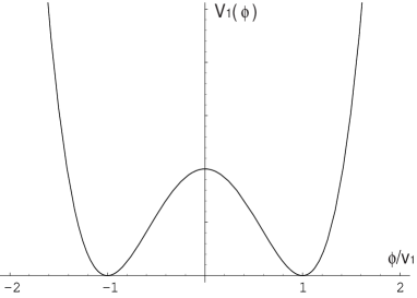
Figure 1: ”Mexican hat” potential $V_{1}$ defined in (51).

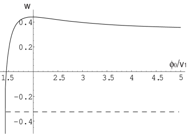
Figure 2: $w$ as a function of the amplitude $\phi_{0}$ of the oscillations in the potential $V_{1}$. The dashed line indicates $w<-1/3$.

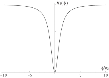
Figure 3: The shape of the potential $V_{2}$ defined in (52).

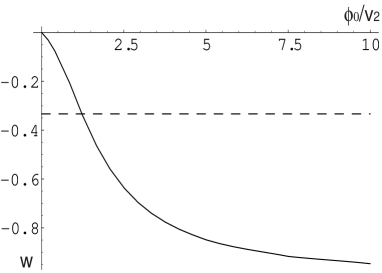
Figure 4: $w$ as a function of the amplitude $\phi_{0}$ of the oscillations in the potential $V_{2}$. The dashed line indicates $w<-1/3$.

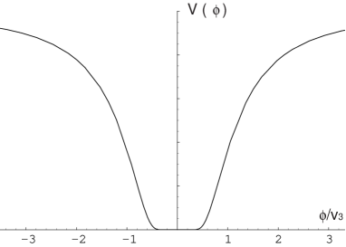
Figure 5: The shape of the potential $V_{3}$ defined in (53).

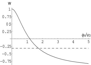
Figure 6: $w$ as a function of the amplitude $\phi_{0}$ of the oscillations in the potential $V_{3}$. The dashed line indicates $w<-1/3$.

References

-
(1)
S. Perlmutter et al. [Supernova Cosmology Project
Collaboration],
Astrophys. J. 517, 565 (1999) [arXiv:astro-ph/9812133].
A. G. Riess et al. [Supernova Search Team Collaboration], Astron. J. 116, 1009 (1998) [arXiv:astro-ph/9805201]. -
(2)
D. N. Spergel et al. ApJS, 148, 175.
A. Balbi et al., Astrophys. J. 545, L1 (2000) [Erratum-ibid. 558, L145 (2001)] [arXiv:astro-ph/0005124].
C. Pryke, N. W. Halverson, E. M. Leitch, J. Kovac, J. E. Carlstrom, W. L. Holzapfel and M. Dragovan, Astrophys. J. 568, 46 (2002) [arXiv:astro-ph/0104490].
C. B. Netterfield et al. [Boomerang Collaboration], Astrophys. J. 571 (2002) 604 [arXiv:astro-ph/0104460].
J. L. Sievers et al., Astrophys. J. 591, 599 (2003) [arXiv:astro-ph/0205387].
A. Benoit et al. [the Archeops Collaboration], Astron. Astrophys. 399, L25 (2003) [arXiv:astro-ph/0210306]. -
(3)
L. Verde et al., Mon. Not. Roy. Astron. Soc. 335 (2002)
432 [arXiv:astro-ph/0112161].
M. S. Turner, The Astrophysical Journal, 576:L101-L104, 2002.
A. Lewis and S. Bridle, Phys. Rev. D 66, 103511 (2002) [arXiv:astro-ph/0205436].
X. m. Wang, M. Tegmark and M. Zaldarriaga, Phys. Rev. D 65, 123001 (2002) [arXiv:astro-ph/0105091]. -
(4)
P. J. E. Peebles and B. Ratra,
Astrophys. J. 325, L17 (1988).
B. Ratra and P. J. E. Peebles, Phys. Rev. D 37, 3406 (1988).
R. R. Caldwell, R. Dave and P. J. Steinhardt, Phys. Rev. Lett. 80, 1582 (1998) [arXiv:astro-ph/9708069].
M. S. Turner and M. J. White, Phys. Rev. D 56, 4439 (1997) [arXiv:astro-ph/9701138].
J. A. Frieman, C. T. Hill, A. Stebbins and I. Waga, Phys. Rev. Lett. 75, 2077 (1995) [arXiv:astro-ph/9505060]. - (5) K. Freese and M. Lewis, Phys. Lett. B 540, 1 (2002) [arXiv:astro-ph/0201229].
- (6) M. S. Turner, Phys. Rev. D 28, 1243 (1983).
-
(7)
H. Goldstein, ”Classical mechanics” (2nd ed.), Addison
Wesley, Reading, MA, 1980.
L. D. Landau and E. M. Lifshitz, ”Mechanics” (3rd ed.), Butterworth-Heinemann, Oxford, 1976.
I. Merches and L. Burlacu, ”Analytical Mechanics and Mechanics of Deformable Media”, Didactic and Pedagogical Publishing House, Bucharest, 1983.
L. Dragos, ”Principles of Analytical Mechanics”, Technical Publishing House, Bucharest, 1976. -
(8)
J. Preskill, M. B. Wise and F. Wilczek,
Phys. Lett. B 120, 127 (1983).
L. F. Abbott and P. Sikivie, Phys. Lett. B 120, 133 (1983).
M. Dine and W. Fischler, Phys. Lett. B 120, 137 (1983). - (9) I. S. Gradshteyn and I. M. Ryzhik, ”Table of Integrals, Series, and Products” (6th ed.), Academic, San Diego, 2000.
- (10) P. B. Greene, L. Kofman, A. D. Linde and A. A. Starobinsky, Phys. Rev. D 56, 6175 (1997) [arXiv:hep-ph/9705347].
- (11) T. Damour and V. F. Mukhanov, Phys. Rev. Lett. 80, 3440 (1998) [arXiv:gr-qc/9712061].
- (12) M. Sami, Grav. Cosmol. 8, 309 (2003) [arXiv:gr-qc/0106074].
- (13) S. D. H. Hsu, Phys. Lett. B 567, 9 (2003) [arXiv:astro-ph/0305096].
- (14) A. R. Liddle and R. J. Scherrer, Phys. Rev. D 59, 023509 (1999) [arXiv:astro-ph/9809272].
- (15) B. Ratra, Phys. Rev. D 44, 352 (1991).