Detached binaries in the Large Magellanic Cloud

As a result of a careful selection of eclipsing binaries in the Large Magellanic Cloud using the OGLE-II photometric database, we present a list of 98 systems that are suitable targets for spectroscopic observations that would lead to the accurate determination of the distance to the LMC. For these systems we derive preliminary parameters combining the OGLE-II data with the photometry of MACHO and EROS surveys. In the selected sample, 58 stars have eccentric orbits. Among these stars we found fourteen systems showing apsidal motion. The data do not cover the whole apsidal motion cycle, but follow-up observations will allow detailed studies of these interesting objects.

1 Introduction

Diverse methods have been employed in the last decade to derive distances to the Magellanic Clouds (see, e.g., Cole cole (1998), Harries et al. harries (2003), Alves alves (2004)). The knowledge of these distances is important for at least two reasons. First, Magellanic Clouds play a key role in the calibration of the Cepheid-based distance scale. Second, due to the low metallicity of the Clouds, it can be checked how different methods used for distance determination depend on metallicity. Unfortunately, as far as the distance moduli of the Magellanic Clouds are concerned, different methods gave results that disagree at a level that leaves in doubt their applicability for more distant objects.

However, the idea of measuring distances by means of eclipsing binaries seems very promising and supposedly will soon succeed in finding the correct answer. The method has been known for many years and first applied to a Magellanic Cloud star by Bell et al. (bell91 (1991)). Its potential usefulness has been recalled a few years ago by Paczyński (paczynski (1997)), while historical outlook was presented by Kruszewski & Semeniuk (krusz (1999)). The method exploits the advantages of a combination of the light curve of an eclipsing binary with its double-lined spectroscopic orbit. This combination provides radii, masses and ratio of surface brightnesses of the components. To get the distance, it is enough to calibrate surface brightness, $F_{\rm V}$, in terms of an easily-observed colour index and account for interstellar extinction. The calibration of $F_{\rm V}$ is usually made using nearby (that is, having accurate parallaxes) eclipsing binaries and/or interferometric and occultation radii of stars (Barnes et al. barnes78 (1978), di Benedetto dibe (1998), van Belle vanbe (1999)).

In order to avoid possible systematic effects on the calibration of $F_{\rm V}$ for close binaries, it was pointed out at the beginning that detached systems (hereafter DEBs) are the best for the purpose of distance determination (e.g. Paczyński paczynski (1997)). However, since alternatively to the application of the calibration of $F_{\rm V}$, the fit of the modern model atmospheres to the UV/optical spectrum can be utilized, the advantage of using only the DEBs is not so straightforward. As was argued by Wyithe & Wilson (WW2 (2002)) and Wilson (wils04 (2004)), semi-detached binaries can be used for the purpose of distance determination as well. Unlike in the DEBs, the photometric mass ratio can be derived, so that a single-lined spectroscopic orbit is sufficient. In addition, current modeling programs describe the proximity effects very well. Moreover, the orbits of semi-detached systems are well circularized, which is not always the case for the DEBs. In fact, out of ten eclipsing systems used by Harries et al. (harries (2003)) to get the distance to the Small Magellanic Cloud (SMC), only three are the DEBs, while six have a semi-detached geometry. Since each binary provides the distance, one can get the average distance with an unprecedented accuracy using as many systems as possible. The ten systems analyzed by Harries et al. (harries (2003)) led to the—so far—best estimation of the SMC distance modulus: 18.89 $\pm$ 0.04 mag with a 0.10-mag uncertainty due to systematic effects. The authors, however, intend to derive the distance of the SMC using over 100 eclipsing binaries.

A similar work is underway for the Large Magellanic Cloud (hereafter LMC). So far, seven systems were used to get its distance. Out of them, only three, HV 2274 (Guinan et al. guinan (1998), Udalski et al. 1998a , Ribas et al. hv2274 (2000), Nelson et al. nelson (2000), Groenewegen & Salaris groen (2001), Fitzpatrick et al. hv982 (2002)), EROS 1044 (Ribas et al. eros1044 (2002)) and HV 982 (Fitzpatrick et al. hv982 (2002), Clausen et al. clausen (2003)), are DEBs. Out of the remaining four, three, i.e. HV 5936 (Bell et al. bell93 (1993), Fitzpatrick et al. fitz03 (2003)), HV 2241 (Pritchard et al. prit98a (1998), Ostrov et al. ostr01 (2001)) and HV 2543 (Ostrov et al. ostr00 (2000)) are semi-detached systems, whereas Sk $-$67^o 105 (Ostrov & Lapasset osla (2003)) is even a contact binary. As indicated above, in order to derive the distance accurately, we need to analyze many more systems.

Fortunately, microlensing surveys delivered photometric measurements for millions of stars in the Clouds and catalogs including thousands of eclipsing binaries were published. First, Grison et al. (grison (1995)) published double-band photometry for 79 eclipsing systems in the LMC bar discovered within the EROS survey. Next, Alcock et al. (alcock (1997)) classified 611 eclipsing binary stars in the LMC from the MACHO survey. Finally, the catalogs of eclipsing binaries from the OGLE-II survey were published: for the SMC (Udalski et al. 1998b , Wyrzykowski et al. wyrz-smc (2004)), and the LMC (Wyrzykowski et al. wyrz-lmc (2003), hereafter W03). In total, about 4500 eclipsing binaries (1914 in the SMC and 2580 in the LMC) were found in the OGLE-II data in both Clouds. Therefore, the first step towards the accurate distance determination to the LMC is good selection of binaries that are suitable for this purpose.

This is the main goal of this paper. Using the photometry obtained during the second phase of the OGLE survey, OGLE-II, we have selected 98 DEBs brighter than 17.5 mag in $V$. We have also analyzed their light curves by means of the Wilson-Devinney (Wilson & Devinney wd (1971), Wilson wils79 (1979), wils90 (1990)) program, combining the photometry from the OGLE-II, MACHO and EROS surveys. The preliminary results of this paper have been presented by Michalska & Pigulski (our-prel (2004)). A list of 36 DEBs in the LMC good for distance determination was presented by W03. A similar selection has been done for the SMC eclipsing binaries by Udalski et al. (1998b ), Wyithe & Wilson (WW1 (2001)), and Graczyk (graczyk (2003)).

The data used in this study are described in Sect. 2. Section 3 presents our selection criteria followed by description of the new transformation of the OGLE-II differential fluxes to magnitudes (Sect. 4). The analysis of the light curves and discussion of the parameters is described in Sect. 5. Finally, we discuss systems with apsidal motion (Sect. 6) and provide our conclusions (Sect. 7).

2 The photometry

2.1 OGLE data

The OGLE observations we used were carried out during the second phase of this microlensing survey (Udalski et al. ogle2 (1997)) with the 1.3-m Warsaw telescope at the Las Campanas Observatory, Chile. They cover about 4.5 square degrees in the LMC bar (twenty one 14^′ $\times$ 57^′ fields). The data span almost four years (1997–2000). This was the primary source of our photometric data used to select the DEBs (Sect. 3). The other databases (MACHO and EROS) were used as supplementary ones.

The OGLE-II photometry for the LMC fields is currently available in three different forms:

• Mean $BVI$ magnitudes for $\sim$7 $\times$ 10⁶ stars (Udalski et al. udal00 (2000)) derived by means of the profile-fitting package DoPhot (Schechter et al. dophot (1993)).

• Time-series $I$-filter photometry of about 53 400 variable candidates published by Żebruń et al. (2001b ). The photometry was obtained by means of the Difference Image Analysis (DIA) package developed by Woźniak (wozniak (2000)) which is an implementation of the image subtraction method of Alard & Lupton (ism (1998)). The photometry is available from the OGLE web page in two forms: as differential fluxes and the magnitudes transformed from these fluxes. The transformation was explained in detail by Żebruń et al. (2001b ).

• $BVI$ time-series photometry for the same variable candidates obtained with DoPhot and available from the same web page. Typically, about 30, 40 and 400 datapoints are available for each star in $B$, $V$ and $I$ bands, respectively.

Since the OGLE data were made in the drift-scan mode (Udalski et al. ogle2 (1997)), for a given frame the average epoch of observation is not the same for all stars. Following the prescription given by Żebruń et al. (2001b ), we applied appropriate corrections. Moreover, the data were phased with the derived orbital period and the outliers were rejected.

2.2 MACHO data

The MACHO observations were obtained in blue (440–590 nm) and red (590–780 nm) bands, rougly coincident with Johnson $V$ and Cousins $R$, respectively. The telescope used was the 1.27-m Great Melbourne Telescope situated at Mount Stromlo, Australia. The MACHO data span almost eight years between 1992 and 2000. The photometry is available through the MACHO web page (Allsman & Axelrod allsman (2001)).

The MACHO data are affected by the presence of a large number of outliers. We therefore rejected them in an iterative process fitting accurately the shape of the light curve in the phase diagram. In addition, a spurious variation of instrumental origin with a 1-yr period was removed prior to the analysis. Then, the heliocentric corrections were applied to the published epochs. Since the latter corresponded to the beginning of exposures, half the exposure time (150 s) was added to the epochs as well.

2.3 EROS data

The EROS observations were made in 1991–1992 with the 0.4-m telescope at La Silla, Chile, in two bands, $B_{\rm E}$ and $R_{\rm E}$, having central wavelengths of 490 and 670 nm, respectively (Grison et al. grison (1995)). Since the latter corresponds roughly to the MACHO red band, we used in our study the photometry made in the $B_{\rm E}$ band only. The epochs of EROS data were published in local time (see Ribas et al. eros1044 (2002)), so that a three-hour correction was added. As for the OGLE and MACHO data, some outliers were removed prior to analysis.

3 Selection of objects

As we pointed out in previous sections, the OGLE-II database of candidate variables (Żebruń et al. 2001b ) was the primary source of the analyzed data and the subject of the main selection process. From this catalog, we first extracted the $I$-filter photometry of those stars that were brighter than 17.5 mag in $V$ and had $V-I<$ 0.5 mag (Fig. 1). For all these stars, the analysis of variance (AoV) periodograms of Schwarzenberg-Czerny (alex (1996)) were calculated. Then, the data were phased with the period corresponding to the frequency of the maximum peak in the periodogram and examined visually. After this check, the star was selected for further analysis if: (i) the light curve indicated it was an EA-type eclipsing binary, presumably a DEB, (ii) the proximity effects were small, (iii) the scatter in the light curve was relatively low.

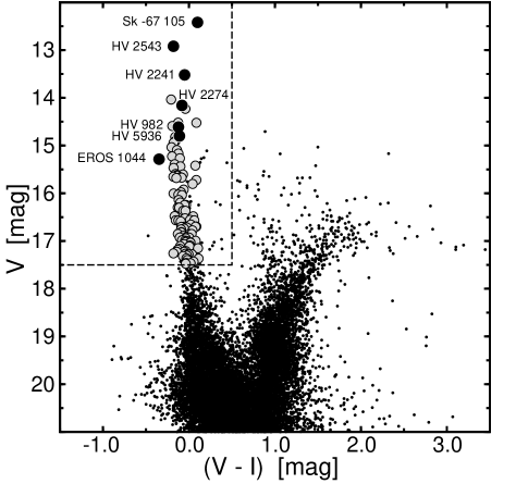
Figure 1: The colour-magnitude diagram for $\sim$16 000 stars from the OGLE-II SC$\_$1 field (small dots). The 98 DEBs we selected as good targets for distance determination are plotted as gray filled circles. For comparison, seven eclipsing binaries already used for the determination of the distance to the LMC are plotted as black filled circles and labeled. The dashed line delimits our selection box.

In total, we found 98 stars that meet our three criteria. For all but five the MACHO photometry is available, eleven are in the list of eclipsing binaries found within the EROS survey. The stars are listed and cross-identified in Table 1.

Our selection was made independently of the work of W03, who—using the same data—discovered 2580 eclipsing binaries, including 1817 of the EA type. It was, however, not our aim to make a complete catalog of eclipsing binaries in the LMC, but to select the brightest DEBs with the best photometry. There are 403 EA-type eclipsing binaries in the catalogue of W03 that fall into the selection box in Fig. 1. Thus, the stars we selected constitute about 25% of this sample. However, three objects from our list, #24, #87, and #91, were not included in the W03 catalogue.

Figure 2: $I$-filter light curves of the OGLE 05223546$-$6931434 (#17) eclipsing binary observed in two fields, LMC_SC5 (circles) and LMC_SC6 (crosses). (a) DoPhot photometry, (b) DIA photometry, (c) DIA photometry with new transformation to magnitudes and a 0.003-mag shift between zero points applied. Note the reduction of scatter in this diagram with respect to the light curve shown in panel (a).

Table 1: List of 98 selected DEBs in the Large Magellanic Cloud. $P_{\rm orb}$ stands for the orbital period. The $VI$ photometry was derived from the OGLE-II DoPhot data and is given for the out-of-eclipse phase at maximum light. In the last column ‘E’ was given for system with non-zero eccentricity and ‘AM’ for systems with detectable apsidal motion. For systems that were indicated as good targets for distance determination by W03, the number is followed by an asterisk. Stars are arranged according to the decreasing $V$ magnitude.

	OGLE	OGLE	MACHO	EROS	$P_{\rm orb}$	$V$	$V-I$
#	field(s)	name	name	name	[d]	[mag]	[mag]	Remarks
1	LMC_SC13	05065201$-$6825466	19.4302.319		6.33000	14.036	$-$0.207	E, AM
2*	LMC_SC2	05303928$-$7014097	7.8147.14		24.673107	14.231	$-$0.041	E
3*	LMC_SC11	05082813$-$6848251	1.4539.37		2.995464	14.520	$-$0.125	E, AM
4*	LMC_SC17	05381862$-$7041084	11.9351.15		2.191363	14.523	0.087
5*	LMC_SC7	05180481$-$6948189	78.6097.13		3.107029	14.591	$-$0.193	E
6*	LMC_SC11	05092929$-$6855028	79.4779.34		2.678832	14.819	$-$0.159	HV 5622, E, AM
7*	LMC_SC16	05351775$-$6943187	81.8881.47		3.881843	14.902	$-$0.156	E, AM
8*	LMC_SC1/16	05350218$-$6944178	81.8881.44		2.989472	14.941	$-$0.178	E
9*	LMC_SC13	05063443$-$6825442	19.4302.345		2.154488	15.036	$-$0.202
10*	LMC_SC7	05182818$-$6937453	78.6220.60	1017	1.403789	15.094	$-$0.139
11*	LMC_SC2	05322529$-$6925374	—		3.370160	15.167	$-$0.122	E
12*	LMC_SC6	05210081$-$6929449	78.6585.50		1.300791	15.227	$-$0.196
13*	LMC_SC15	05014027$-$6851060	1.3449.27		4.034834	15.267	$-$0.105	E, AM
14*	LMC_SC5	05224434$-$6931435	78.6827.52		2.150539	15.391	$-$0.166
15	LMC_SC18	05404706$-$7036564	11.9836.21		7.087663	15.420	0.075
16*	LMC_SC9	05134140$-$6932455	—		5.457320	15.437	$-$0.099	E
17*	LMC_SC5/6	05223546$-$6931434	78.6827.66	1036	2.183363	15.469	$-$0.178
18*	LMC_SC7	05185897$-$6935495	78.6221.90	1074	9.144018	15.596	$-$0.155	E
19*	LMC_SC16	05371417$-$7020015	11.9235.33		3.256696	15.606	$-$0.069	HV 5963, E
20*	LMC_SC8	05164453$-$6932333	78.5859.100	1066	5.603540	15.624	$-$0.143	E
21*	LMC_SC10	05102875$-$6920480	5.4894.3904		3.773443	15.632	$-$0.133	E, AM
22	LMC_SC8	05170507$-$6945234	78.5977.2715		2.864425	15.653	$-$0.180	E
23*	LMC_SC11	05093433$-$6854259	79.4779.81		1.462906	15.663	$-$0.100
24	LMC_SC13	05064333$-$6836115	19.4300.349		4.018698	15.672	$-$0.084	E, AM
25	LMC_SC5	05225771$-$6935094	78.6947.2732		10.187024	15.680	$-$0.146
26*	LMC_SC18	05410194$-$7005047	76.9844.26		2.385189	15.722	0.086
27*	LMC_SC9	05132398$-$6922492	5.5377.4567		2.636570	15.804	0.043	E
28	LMC_SC10	05110289$-$6913098	79.5017.83		2.152919	15.923	$-$0.061
29	LMC_SC6/7	05195816$-$6928239	78.6465.173	1012	1.338312	15.979	$-$0.092
30	LMC_SC4	05251673$-$6929039	77.7312.90		3.288241	16.005	$-$0.178
31	LMC_SC1	05345582$-$6943100	81.8881.97		1.601593	16.028	$-$0.122
32	LMC_SC11	05081572$-$6929044	5.4529.1362		2.899285	16.039	$-$0.081	HV 5619
33	LMC_SC9	05133633$-$6922416	5.5377.4656		2.108729	16.140	$-$0.119	E, AM
34	LMC_SC5	05233948$-$6943346	77.7066.333		2.145747	16.194	$-$0.100
35	LMC_SC15	05000218$-$6931561	17.3197.781		3.317560	16.245	$-$0.034	E
36	LMC_SC11	05095412$-$6853046	79.4780.100		16.930492	16.247	$-$0.051	E
37	LMC_SC14	05050424$-$6857588	1.4052.2379		9.844484	16.299	$-$0.130	E
38	LMC_SC8	05152057$-$6852502	79.5627.88		1.538050	16.301	$-$0.113
39	LMC_SC4/5	05250946$-$7004226	77.7303.152		3.625522	16.364	$-$0.066	E
40	LMC_SC18	05404159$-$6959014	76.9845.63		2.009981	16.367	$-$0.040	E
41	LMC_SC6	05221179$-$6928551	78.6828.213		7.544703	16.479	$-$0.166	E
42	LMC_SC5	05250140$-$6955086	77.7184.162		8.013626	16.482	0.050	E
43	LMC_SC15	05010991$-$6904496	18.3325.230		9.771474	16.525	$-$0.045	E
44	LMC_SC19	05425713$-$7009580	76.10205.471		7.229139	16.557	0.014	E
45	LMC_SC6	05213496$-$6925346	78.6708.180		2.598897	16.565	$-$0.152	E, AM
46	LMC_SC2	05315853$-$6955320	—		2.918065	16.567	0.063	E
47	LMC_SC13	05053815$-$6820531	19.4062.914		5.621099	16.569	$-$0.122	E
48	LMC_SC13	05072467$-$6829325	19.4423.464		1.672507	16.589	$-$0.095
49	LMC_SC9	05130842$-$6908018	79.5260.94		1.240540	16.655	0.022
50	LMC_SC10	05121954$-$6914547	79.5137.189		8.523814	16.697	0.086	E
51	LMC_SC4	05265371$-$6959493	77.7546.303		2.431105	16.700	0.077
52	LMC_SC4	05263667$-$6951253	77.7548.325		2.503626	16.702	$-$0.059	E, AM
53	LMC_SC9	05134039$-$6918217	79.5378.261		0.956442	16.704	$-$0.088
54	LMC_SC4	05263256$-$6945127	—	1037	2.233238	16.718	$-$0.023

Table 1: Continued.

	OGLE	OGLE	MACHO	EROS	$P_{\rm orb}$	$V$	$V-I$
#	field(s)	name	name	name	[d]	[mag]	[mag]	Remarks
55	LMC_SC9	05130354$-$6917122	79.5258.87		3.289306	16.740	$-$0.055
56	LMC_SC9	05143268$-$6912269	79.5501.310		1.232396	16.757	$-$0.091
57	LMC_SC7	05174797$-$6904161	—		3.954434	16.777	0.041
58	LMC_SC7	05174804$-$6945493	78.6097.233		5.231974	16.814	$-$0.088	E
59	LMC_SC14	05025511$-$6853029	1.3691.210		2.789120	16.821	$-$0.089	E, AM
60	LMC_SC21	05222806$-$7022407	6.6814.103		5.376945	16.852	0.008	E
61	LMC_SC4	05263908$-$6936060	77.7552.249		3.932107	16.852	$-$0.128	E
62	LMC_SC17	05383042$-$6949483	81.9484.91		4.261134	16.853	0.031	E, AM
63	LMC_SC1	05324193$-$6951092	81.8516.176		4.954343	16.892	$-$0.064	E, AM
64	LMC_SC4	05260950$-$6959109	77.7425.249		17.366232	16.917	$-$0.027	E
65	LMC_SC9	05132215$-$6927252	5.5376.2159		1.788358	16.927	$-$0.106
66	LMC_SC6	05222482$-$6936226	78.6826.298	1041	2.688218	16.929	0.003	E
67	LMC_SC2	05312473$-$6925281	77.8281.58		2.536663	16.944	$-$0.036	E
68	LMC_SC11	05092769$-$6856194	79.4658.4032		1.827980	16.983	$-$0.079
69	LMC_SC3	05285710$-$6948441	77.7912.282		6.069953	16.992	$-$0.044
70	LMC_SC9	05142797$-$6854210	79.5505.198		9.002650	16.995	0.078	E
71	LMC_SC5	05224192$-$7006480	6.6818.283		4.210379	17.001	$-$0.023
72	LMC_SC6	05201732$-$7000440	6.6457.4965		2.116275	17.021	$-$0.036
73	LMC_SC14	05041689$-$6849509	1.3812.152		5.280710	17.029	0.016	E
74	LMC_SC9	05133011$-$6908412	79.5381.199		9.503056	17.036	0.018	E
75	LMC_SC3	05292500$-$6948081	77.7912.709		1.966261	17.067	$-$0.058
76	LMC_SC13	05062656$-$6857153	1.4174.183		5.322229	17.094	0.013	E
77	LMC_SC6	05211299$-$6950512	78.6580.255		2.160515	17.107	$-$0.101	E
78	LMC_SC10	05121869$-$6858325	79.5141.200		2.390521	17.113	0.005	E
79	LMC_SC10	05122789$-$6920513	5.5257.3679		1.982183	17.151	0.106
80	LMC_SC9	05140857$-$6923003	5.5498.5030		1.628412	17.164	$-$0.107
81	LMC_SC7	05181228$-$6936251	78.6100.388	1061	4.538132	17.182	$-$0.131	E
82	LMC_SC1	05331282$-$7007025	81.8512.224		5.394376	17.211	$-$0.037	E
83	LMC_SC5/6	05223386$-$6932564	78.6827.465		1.284099	17.224	$-$0.145
84	LMC_SC6	05221500$-$6938483	78.6825.430	1063	4.722907	17.226	$-$0.055	E
85	LMC_SC6	05203518$-$6934378	78.6463.505		2.117483	17.226	$-$0.142	E
86	LMC_SC6	05222499$-$6938103	78.6825.431	1053	3.570088	17.259	$-$0.180	E
87	LMC_SC8	05170646$-$6940570	78.5978.403		1.635801	17.268	$-$0.042
88	LMC_SC10	05112066$-$6909148	79.5018.187		1.345239	17.278	0.035
89	LMC_SC10	05115154$-$6920494	79.5136.250		1.760103	17.280	$-$0.005	E, AM
90	LMC_SC4	05264527$-$6944045	77.7550.352		6.536197	17.304	$-$0.024	E
91	LMC_SC7	05181122$-$6932555	78.6101.407		3.816795	17.317	$-$0.069
92	LMC_SC6	05222991$-$6919090	80.6830.375		6.310800	17.363	$-$0.028	E
93	LMC_SC1	05335582$-$7019049	11.8630.374		4.568919	17.368	0.112
94	LMC_SC9	05145023$-$6915416	79.5621.470		4.670019	17.399	$-$0.018
95	LMC_SC2	05323120$-$6928535	81.8522.169		4.897253	17.431	0.054	E
96	LMC_SC7	05181271$-$6935245	78.6100.606	1039	2.575579	17.460	$-$0.032	E
97	LMC_SC6	05221305$-$7003284	78.6819.336		2.138851	17.466	0.019	E
98	LMC_SC14	05025406$-$6918398	1.3684.237		3.825716	17.475	$-$0.037

4 New transformation to magnitudes

As mentioned in Sect. 2.1, two sources of time-series data in the $I$ filter expressed in magnitudes are available from the OGLE-II survey. At the beginning, we had to decide which of them use in the subsequent analysis. Due to the crowded nature of the LMC fields, the DIA photometry has considerably smaller scatter than that obtained by means of profile fitting and hence it seems to be preferable. However, this photometry suffers from the unavoidable bias occuring during the transformation from differential fluxes to magnitudes (see, e.g., Woźniak wozniak (2000) or Żebruń et al. 2001a ). The bias in the transformed magnitude, $m_{\rm DIA}$, comes mainly from the uncertainty of the reference flux, $f_{\rm ref}$, in the transformation equation:

$$m_{\rm DIA}=-\mbox{2.5}\log(f_{\rm ref}+\Delta f)+C.$$ (1)

In the above equation, $\Delta f$ denotes differential flux, and $C$ is the zero point of the magnitude scale. While the uncertainty in $C$ does not affect the shape and the magnitude range of the transformed light curve, that of $f_{\rm ref}$ does. In consequence, the parameters derived from the fit of the light curve would be affected as well.

The problem is illustrated in Fig. 2 for a star that was observed within OGLE-II in two overlapping fields. The top panel shows the light curve derived by means of DoPhot. The light curves from the two fields agree quite well, there is only a small 0.003-mag shift in the mean brightness between them. On the other hand, the DIA light curves (middle panel) are less scattered, but one is shifted by $\sim$0.1 mag with respect to the other and the eclipses have slightly different depths. This is because $f_{\rm ref}$ was derived merely from the profile-fitting in the reference images. The reference images, although obtained by co-adding 20 best frames in each field (Żebruń et al. 2001a ), were still quite crowded. Therefore, we calculated new $f_{\rm ref}$ and $C$ values in Eq. (1), fitting the DIA differential fluxes to the DoPhot magnitudes by means of least-squares fits. The result is shown in Fig. 2c. This approach combines the advantages of both photometries: small scatter of the DIA photometry and the correct range in brightness of the DoPhot one. A new transformation was derived for all eclipsing binaries selected for further analysis. Although the example shown in Fig. 2 is an extreme rather than a typical case, we encourage all users of the DIA photometry to do a new transformation in all applications where the correct magnitude scale is required.

5 Analysis of light curves

The light curves in three (or four, if the EROS $B_{\rm E}$ photometry was available) bands, MACHO blue and red, (designated thereafter $V_{\rm M}$ and $R_{\rm M}$, respectively) and OGLE $I$, were analyzed simultaneously by means of the improved version of the Wilson-Devinney (WD) program that includes a model atmosphere routine developed by Milone et al. (milone (1992)). The program is composed of the LC program generating light curves for assumed parameters and the differential correction program, DC. The WD program was used in two different ways: (1) to search the space of the adjustable parameters by means of the Monte-Carlo method with the LC program, (2) to get the best-fit solution for a given system with the DC one.

5.1 Assumptions

The DC program allows adjusting of over thirty parameters. In practice, only a few are adjusted since the remaining are either known quite well or cannot be reliably obtained from the fit. The choice of adjustable parameters have to be decided first.

Since the components of the DEBs are roughly spherical in shape, it is not possible to get the mass ratio, $q=M_{2}/M_{1}$, solely from the analysis of the light curves (Wyithe & Wilson WW1 (2001)). Michalska & Pigulski (our-prel (2004)) presented an example showing that equally good fits can be obtained in a very large range of mass ratios. It is therefore reasonable to assume $q$ = 1, as we did in this analysis, although it is obvious that for systems with unequal minima, $q$ might be far from unity. The WD program was run with detached geometry (MODE = 2), as the selected stars were suspected to be DEBs. If, however, the gravitational potential of one of the components appeared to be close to the critical one, the system was excluded from the analysis.

The choice we made in Sect. 3 allowed us to assume safely that the components of the analyzed systems were early-type main-sequence stars. Consequently, we assumed bolometric albedos and gravity darkening coefficients equal to 1.0, a value typical for stars with radiative envelopes. The logaritmic limb darkening law (LD = 2) with coefficients taken from van Hamme (hamme (1993)) for $\log g$ = 4.0 was adopted. In addition, we assumed synchronous rotation and no spots. As far as the reflection effect is concerned, a detailed reflection model with two reflections (MREF = 2 and NREF = 2) was assumed for systems with circular orbits. For eccentric systems a simpler model with single reflection (MREF = 1 and NREF = 1) was adopted. This difference is not important as the reflection effect is never significant for the systems we selected.

The major semi-axis of the relative orbit, $a$, has little to do with the light curve. However, since even an estimation gives an idea of the expected range of radial velocities, we tried to evaluate $a$. At the beginning, it was assumed to be equal to 25 $R_{\odot}$. Once the masses of the components were estimated (see below), $a$ was calculated from the generalized Kepler’s law.

The effective temperature of the primary component, $T_{1}$, is the last important parameter that needs to be assumed. In order to do this in a consistent way, we employed an iterative procedure shown schematically in Fig. 3. Using the out-of-eclipse $V$ magnitudes, we first estimated the absolute magnitude of the primary, $M_{\rm V}$, according to the equation:

$$M_{\rm V}=V-DM-A_{\rm V}-\mbox{2.5}\log\frac{L_{1}}{L_{1}+L_{2}},$$ (2)

where the average values for the LMC distance modulus, $DM$ = 18.5 mag, and total extinction, $A_{\rm V}$ = 0.3 mag, were assumed. The component’s monochromatic luminosities were first assumed to be the same, $L_{1}$ = $L_{2}$, then they were taken from the DC output (see Fig. 3). Having calculated $M_{\rm V}$, the bolometric magnitude, $M_{\rm bol}(M_{\rm V})$ relation in a form of a sixth-order polynomial was derived using the bolometric corrections published by Popper (popper (1980)). The coefficients, $a_{n}$, of the polynomial

$$P(A)=\sum\limits_{n=0}^{N}a_{n}A^{n},$$

are given in Table 2.

Figure 3: The scheme of the procedure aimed in estimating the effective temperature of the primary, $T_{1}$. See Sect. 5.1 for details.

Table 2: The coefficients of the polynomials in the relations (3)–(5). $P$ is a parameter, $A$, the argument of a relation.

Eq.	(3)	(4)	(5)
$P(A)$	$M_{\rm bol}(M_{\rm V})$	$\log M_{1}(M_{\rm bol})$	$\log T_{1}(M_{\rm bol})$
$N$	6	4	6
$a_{0}$	$-$1.46072	0.468944	4.07891
$a_{1}$	1.67977	$-$9.46798 $\cdot$ 10-2	$-$8.02904 $\cdot$ 10-2
$a_{2}$	1.94271 $\cdot$ 10-2	$-$4.76657 $\cdot$ 10-4	$-$1.69451 $\cdot$ 10-3
$a_{3}$	$-$3.00150 $\cdot$ 10-2	$-$1.16486 $\cdot$ 10-4	1.16818 $\cdot$ 10-3
$a_{4}$	$-$1.53159 $\cdot$ 10-3	4.00185 $\cdot$ 10-5	9.66154 $\cdot$ 10-5
$a_{5}$	1.07280 $\cdot$ 10-3	…	$-$3.35212 $\cdot$ 10-5
$a_{6}$	$-$7.38667 $\cdot$ 10-5	…	$-$3.48540 $\cdot$ 10-6

The coefficients of the effective temperature vs. luminosity, $\log T_{1}(M_{\rm bol})$, and mass-luminosity, $\log M_{1}(M_{\rm bol})$ relations, are also given in Table 2. They were derived from the data published for Galactic detached main-sequence eclipsing binaries by Harmanec (harmanec (1988)). In order to account for smaller metallicity of the LMC, we applied a correction taken from the comparison of stellar parameters for $Z$ = 0.02 and $Z$ = 0.008 models of Bertelli et al. (bertelli (1994)) for the youngest stars ($\log({\rm age/year})$ = 6.6, $M_{1}<$ 15 $M_{\odot}$).

5.2 Adjusted parameters

The adjusted parameters were the following:

• phase shift, $\phi_{0}$,

• surface potentials, $\Omega_{1}$ and $\Omega_{2}$,

• effective temperature of the secondary component, $T_{2}$,

• inclination, $i$,

• luminosity of the primary component, $L_{1}$.

For a few systems (#21, #28, #29, #32, #66, #73, #81, and #88) it was necessary to include into the solution the third light, $L_{3}$, as an additional adjustable parameter. The DC program provides also the fractional radii, $r_{1}$ and $r_{2}$ (back, pole, point, and side), and the luminosity of the secondary, $L_{2}$. After a first guess of the parameters, the procedure shown in Fig. 3 was repeated five times. Then, $a$ and $T_{1}$ were fixed and the iterations were repeated until the solution converged. In order to scrutinize the solution, we utilized the Monte-Carlo method (Sect. 5.3) that warrants finding a global minimum in the parameter space.

Figure 4: Results of the M-C simulations for three DEBs with different light-curve morphology. Left: Light curves of #83 (complete eclipses, similar components), #88 (complete eclipses, different components, and #49 (partial eclipses). The ordinate range is the same for all three stars and equals to 1 mag. Right: Panels showing the dependencies between $i$, $T_{2}/T_{1}$, $\Omega_{1}$ and $\Omega_{2}$. The ranges of the parameters are the same as labeled at the top. The contours we show encompass all solutions with SSR smaller than $A$ $\cdot$ SSR_min, for four values of $A$: 2, 1.73, 1.41, and 1.22. The WD and M-C solutions are plotted as dots and crosses, respectively, with error bars.

5.3 Monte-Carlo simulations

The Monte-Carlo (M-C) method is often used in problems with a complicated parameter space and strong correlations between parameters. It also provides an independent way to estimate the uncertainties of the parameters in the presence of the mentioned correlations.

The preliminary solution, obtained by means of the WD program, was used to define the ranges of parameters that were searched for the best solution. The parameters were the same as listed in Sect. 5.2, except for $\phi_{0}$ that was fixed at the value obtained during the DC iterations. The synthetic light curves were calculated using the LC program with a randomly-generated (within a defined range) set of parameters. The weighted sum of squares of the residuals (hereafter SSR) was stored as the goodness-of-fit estimator. At this stage we faced the problem of whether to compare the synthetic and observed light curves in all available bands and combine the resulting weighted SSRs to get a general estimation of the multi-band solution or do the same for a single band. The first approach has the advantage of being able to discriminate better solutions in case of unequal components. However, when the components are similar and there are large differences in the scatter between different bands, a single band determined the shape of the minimum in the parameter space. For that reason we decided to follow the second approach (single band), choosing the band with the smallest scatter in photometry. The band we chose is indicated in the last column of Table 3. Only in a few cases, when the scatter was similar in two bands, we did trial M-C simulations for these two bands separately and then compared the results. The global solutions obtained with the M-C method appeared to be consistent with the preliminary ones for all but a few systems.

Some examples of the results of the M-C simulations are shown in Fig. 4 for three systems with different light-curve morphology. In this figure, we plot contours that encompass all solutions with SSR smaller than a certain value expressed in terms of the minimum value of SSR. Let us first comment on the $\Omega_{2}$ vs. $\Omega_{1}$ panels, as the surface potentials decide how well the components’ dimensions are constrained. We see that $\Omega$s are best constrained for a system with complete eclipses and components that are not similar (#88). In the case of similar components (#83) we can also get $\Omega$s, but there are two alternative solutions. This is obvious, as the same components in a circular orbit produce eclipses indistinguishable in shape. Wyithe & Wilson (WW1 (2001)) call these solutions ‘aliasing’. For partial eclipses (#49), the solutions spread over a crescent-shaped area that is quite wide in both $\Omega$s. This is understandable as the change in $\Omega$ can be easily compensated by change of inclination. The relative radii for a system with partial eclipses is therefore much poorly constrained. In general, this means that such systems are much less suitable for the distance determination.

Figure 5: Parameters of 98 systems selected in this paper. For comparison, the same parameters are also plotted (as asterisks) for the seven systems listed in the Introduction that were already used to derive the distance of the LMC. Left: Sum of relative radii, $r_{1}+r_{2}$ (a), $F_{\rm e}$ parameter (b), and ratio of effective temperatures, $T_{2}/T_{1}$, plotted against the $V$ magnitude. Parameters for systems with circular orbits are plotted as filled circles, for eccentric systems, as open circles, and the eccentric systems with detected apsidal motion, as encircled dots. Right: Sum of the relative radii, $r_{1}+r_{2}$ (d), and eccentricity, $e$ (e), plotted as a function of the orbital period. The same symbols as in panels (a)–(c) are used. The (f) panel shows the $e$ vs. $\omega$ (longitude of periastron) dependence. Systems with apsidal motion are plotted as encircled dots.

5.4 Discussion of solutions

Table 3 lists the parameters of 98 systems derived by means of the WD program. For 84 stars from this sample we also provide the results obtained with the M-C simulation. The remaining fourteen eccentric systems show a detectable apsidal motion and the M-C simulation was not performed for these stars. They are discussed separately in Sect. 6.

Since, as shown above, surface potentials are not well constrained for the DEBs, we instead provide in Table 3 the sum of relative radii, $r_{1}+r_{2}$. In addition, the $F_{\rm e}$ parameter is given, defined by Wyithe & Wilson (WW1 (2001)) as:

$$F_{\rm e}=\frac{r_{\rm 1}+r_{\rm 2}-\cos i}{2r_{\rm 2}},$$ (3)

where $r_{\rm 1}$ and $r_{\rm 2}$ denote the fractional radii (in terms of the relative distance during the eclipse) of the larger and smaller star, respectively. For systems with total eclipses, $F_{\rm e}\geq$ 1. However, the denominator of (3) is not well known, so that the values of $F_{\rm e}$ we provide should be treated with caution. In the case of an eccentric orbit, the relative distance can be different in both eclipses. For this reason we list two values of $F_{\rm e}$ in Table 3. Finally, the range of radial velocities, resulting from the derived parameters, masses of the components and dimensions estimated in Sect. 5.1, are given in the tenth column of Table 3. This is a rough estimation, but it can be useful in view of the future spectroscopic observations.

The parameters of the systems are also shown in Fig. 5a-f. As a result of the application of the selection criteria (Sect. 3), we deal mostly with systems that have similar components. This can be seen in Fig. 5c: for most systems 0.8 $<T_{2}/T_{1}<$ 1.0, with only a few stars outside this range. From Fig. 5a and 5d we see that the closest systems (i.e., having largest $r_{1}+r_{2}$) have—as expected—mostly circular orbits and shortest periods. For $r_{1}+r_{2}\geq$ 0.5 all orbits are circularized, which is consistent with the results of North & Zahn (noza (2003)). Practically all systems with $P_{\rm orb}$ shorter than $\sim$2 d have circularized orbits. This is a value typical for early-type, i.e., young systems, but much shorter than in older populations (Mathieu & Mazeh mama (1988)).

Figure 6: The $O$ $-$ $C$ diagrams for fourteen systems with apsidal motion. The filled and open circles denote the primary and secondary times of minimum, respectively. Note different ordinate scales.

6 Systems with apsidal motion

As a consequence of the tidal and rotational distortions, the apsidal motion is observed in some eccentric systems. With the aid of theory, the knowledge of the rate of apsidal motion can be used to test the internal structure of the binary components (Claret & Giménez clgi93 (1993), Claret claret (1999) and references therein) or even derive their masses (Benvenuto et al. benv02 (2002)). We detected that fourteen eccentric systems listed in Table 1 exhibit measurable apsidal motion. Since the WD program allows fitting of the rate of change of the longitude of periastron, $\dot{\omega}$ = $d\omega/dt$, we derived these values from the WD fits. They are listed in the fourth column of Table 4. The values of $e$ and $\omega$ are repeated from Table 3 for reference. Note that for systems with apsidal motion, $\omega$ is given for epoch HJD 2450500.0.

Table 4: Parameters for 14 systems with apsidal motion detected. The values of $e$ and $\omega$ were repeated from Table 3. The remaining parameters are explained in the text.

Star	$e$	$\omega$	$\dot{\omega}$	$P_{\rm mean}$	$T_{\rm 0,\,mean}$
		[o]	[o/year]	[d]	[HJD 244…]
#1	0.358	74	0.86 $\pm$ 0.04	6.33000	9146.1025
#3	0.036	283	6.9 $\pm$ 1.0	2.995459	9041.9927
#6	0.033	254	7.2 $\pm$ 0.8	2.6788316	9009.9189
#7	0.271	261	2.35 $\pm$ 0.06	3.881843	9153.4719
#13	0.282	282	2.35 $\pm$ 0.04	4.034834	8890.6211
#21	0.215	295	3.05 $\pm$ 0.07	3.773443	9106.6226
#24	0.157	285	2.05 $\pm$ 0.10	4.018700	9209.9996
#33	0.037	280	8.7 $\pm$ 0.7	2.1087292	9114.7029
#45	0.089	60	3.64 $\pm$ 0.28	2.5988972	9153.9262
#52	0.108	114	3.31 $\pm$ 0.23	2.503626	9030.7418
#59	0.053	106	3.2 $\pm$ 0.4	2.7891195	9022.6667
#62	0.296	248	1.21 $\pm$ 0.06	4.261134	9102.1955
#63	0.365	265	0.79 $\pm$ 0.03	4.954343	9187.7252
#89	0.052	71	5.9 $\pm$ 0.6	1.7601028	9041.5233

The $O$ $-$ $C$ diagrams for the 14 systems under consideration are shown in Fig. 6. They were obtained in the following way. First, the MACHO blue and OGLE-II data were divided into five to thirteen subsets, depending on the star. Then, the WD program was run separately for each subset with $e$ and $\omega$ fixed. The phase of primary and secondary minimum was next derived from the fit. These phases were transformed into times of minimum closest to the mean epoch of all observations in a given subsample.

Having obtained the times of minimum from all subsets, we calculated the number of elapsed cycles, $E$, for each minimum and then fitted them with a function

$$T_{\rm min}=T_{0}+P\times E$$

deriving $T_{0}$ and $P$, separately for the primary and secondary ones. A mean of both periods, $P_{\rm mean}$ = ($P_{\rm prim}$ + $P_{\rm sec})/$2, is given in Table 4. We have also averaged the initial epochs; the mean initial epoch $T_{\rm 0,\,mean}$ given in Table 4 was equal to the average of $T_{0}^{\rm prim}$ and $T_{0}^{\rm sec}$ + $P_{\rm mean}/$2. Using the observed epochs, the values of $P_{\rm mean}$ and $T_{\rm 0,\,mean}$, we calculated the $O$ $-$ $C$ values plotted in Fig. 6, where the calculated epochs $C$ were derived from the equation

$$C=T_{\rm 0,\,mean}+P_{\rm mean}\times E$$ (4)

for the primary and

$$C=T_{\rm 0,\,mean}+P_{\rm mean}\times(E+0.5)$$ (5)

for the secondary minima.

As can be seen in Fig. 5e, systems with detected apsidal motion tend to group around $\omega\sim$90^o and 270^o. This is clearly an observational selection effect as in these configurations the effect on the position of the observed minima is largest. The $\dot{\omega}$ values are not determined very accurately (Table 4), but they can be used to estimate the apsidal periods, $U$ = 360${}^{\rm o}/\dot{\omega}$. The values of $U$ are generally longer than $\sim$40 years. The lack of systems with shorter $U$ can be understood as we selected only the DEBs. In DEBs the tidal effects are not as strong as in the systems with closer components for which $U$ is sometimes very short (Petrova & Orlov peor (1999)).

The systems with apsidal motion we found are not the first known in the LMC. Apsidal motion was detected in HV 2274 by Watson et al. (watson (1992)) and thereafter studied by Claret (clar96 (1996)). It was also found in another well-studied DEB in the LMC, HV 982 (Clausen et al. clausen (2003)). In addition, Bayne et al. (bay04 (2004)) recently detected this effect in the LMC system MACHO 05:36:48.7$-$69:17:00 = 82.9130.25.

7 Conclusions

We have selected 98 detached systems in the LMC that have good photometry available. They were extracted from the OGLE-II, MACHO and EROS databases and combined. For the OGLE-II data we performed transformations from fluxes to magnitudes, ensuring both small scatter and the correct range of changes. The next step towards the determination of the distance to the LMC is to obtain radial velocities for at least some of these stars. Since they all are relatively bright, this could be achieved even with 4-m class telescopes.

For all systems we derived astrophysical parameters that could be obtained from the fitting of the light-curve. They can be used to select the targets for spectroscopic observations. Comparison of the parameters of systems that were already used to derive the distance to the LMC with those we select in this paper (Fig. 5) indicates clearly that among the latter there are many systems that are suitable for this purpose.

Special attention should be paid to the fourteen systems in which we detected apsidal motion. Fortunately, OGLE-III continues to observe the LMC, so that we can expect that they may be studied in the future in a much more detail.

Table 3: Parameters of the 98 selected systems. If two lines are presented for a given star, the first one refers to the results of the WD fitting, the other, to the M-C simulations. The errors given for the M-C simulations correspond to the 10% increase of the SSR with respect to the minimum value. The columns are the following: (1), sequential number, (2) effective temperature of star 1 [K] (assumed, see Sect. 5.1), (3) effective temperature of star 2 [K], (4) inclination [^o], (5) sum of relative radii, $r_{1}+r_{2}$, (6),(7) $F_{\rm e}$ parameter; in case of eccentric orbits, two values are given: first corresponds to the primary, the other, to the secondary eclipse, (8) eccentricity, (9) longitude of periastron [^o], (10) estimated semi-amplitude of the radial-velocity changes [km s^-1], (11) filter indicating the data used in the M-C simulations, ‘O’, OGLE-II, ‘MR’, MACHO red, ‘MB’, MACHO blue.

#	$T_{1}^{*}$	$T_{2}$	$i$	$r_{1}+r_{2}$	$F_{\rm e,1}$	$F_{\rm e,2}$	$e$	$\omega$	$K_{1,2}$	M-C
	[K]	[K]	[o]					[o]	[km s-1]	filter
(1)	(2)	(3)	(4)	(5)	(6)	(7)	(8)	(9)	(10)	(11)
1	30900	36260±260	81.1±0.1	0.324±0.002	0.74±0.01	0.42±0.01	0.358±0.005	73.5±0.3	183
2	30410	29310±210	89.3±0.2	0.144±0.001	1.27±0.02	1.21±0.04	0.500±0.001	144.6±0.2	126
		28740${}^{+1810}_{-1170}$	89.8${}^{+0.1}_{-1.6}$	0.144${}^{+0.007}_{-0.004}$	1.30${}^{+0.04}_{-0.19}$	1.29${}^{+0.05}_{-0.30}$				O
3	35560	32510±200	77.1±0.1	0.445±0.003	0.53±0.01	0.57±0.01	0.036±0.004	283±2	240
4	33040	29490±120	75.3±0.1	0.486±0.003	0.49±0.01		0	…	250
		29220${}^{+1560}_{-1740}$	75.0${}^{+1.9}_{-1.3}$	0.485${}^{+0.025}_{-0.030}$	0.48${}^{+0.13}_{-0.03}$					MR
5	34120	32760±90	77.5±0.1	0.461±0.002	0.53±0.01	0.54±0.01	0.042±0.001	337±3	229
		32660${}^{+1130}_{-670}$	77.3${}^{+0.9}_{-0.5}$	0.463${}^{+0.009}_{-0.013}$	0.53${}^{+0.08}_{-0.03}$	0.54${}^{+0.08}_{-0.03}$				O
6	32430	25170±100	80.2±0.1	0.422±0.002	0.63±0.01	0.65±0.01	0.033±0.003	254±2	235
7	32580	30880±150	84.9±0.1	0.341±0.002	0.77±0.01	0.93±0.01	0.271±0.005	260.9±0.2	219
8	25060	18070±100	83.5±0.2	0.377±0.001	1.09±0.02	1.17±0.01	0.099±0.004	307±2	195
		17600${}^{+970}_{-930}$	84.1${}^{+2.9}_{-1.8}$	0.368${}^{+0.019}_{-0.019}$	1.11${}^{+0.24}_{-0.13}$	1.18${}^{+0.21}_{-0.12}$				O
9	28120	26780±180	78.6±0.1	0.511±0.004	0.62±0.01		0	…	229
		29080${}^{+1170}_{-1080}$	78.8${}^{+1.9}_{-0.5}$	0.512${}^{+0.011}_{-0.025}$	0.63${}^{+0.18}_{-0.03}$					O
10	29310	27560±100	71.5±0.1	0.595±0.003	0.47±0.01		0	…	262
		28000${}^{+690}_{-1270}$	71.5${}^{+1.0}_{-0.7}$	0.595${}^{+0.011}_{-0.016}$	0.48${}^{+0.04}_{-0.03}$					O
11	26420	25090±120	89.3±1.2	0.510±0.001	1.15±0.05	1.15±0.05	0.014±0.002	220±10	194
		24940${}^{+830}_{-820}$	89.8${}^{+0.2}_{-3.4}$	0.513${}^{+0.013}_{-0.014}$	1.17${}^{+0.03}_{-0.14}$	1.17${}^{+0.03}_{-0.14}$				O
12	28710	28340±160	70.9±0.1	0.584±0.006	0.44±0.01		0	…	265
		27980${}^{+1250}_{-1230}$	70.7${}^{+1.3}_{-1.1}$	0.592${}^{+0.013}_{-0.023}$	0.44${}^{+0.06}_{-0.02}$					O
13	29380	28350±120	84.1±0.1	0.335±0.002	0.71±0.01	0.89±0.01	0.282±0.004	281.5±0.1	202
14	27420	26060±110	72.8±0.1	0.530±0.003	0.45±0.01		0	…	220
		26020${}^{+1140}_{-1700}$	73.1${}^{+1.3}_{-1.3}$	0.527${}^{+0.021}_{-0.024}$	0.46${}^{+0.08}_{-0.03}$					MB
15	26980	26960±200	81.8±0.1	0.245±0.002	0.50±0.01		0	…	152
		27060${}^{+2080}_{-2900}$	81.5${}^{+4.7}_{-1.1}$	0.258${}^{+0.025}_{-0.051}$	0.42${}^{+0.76}_{-0.04}$					MR
16	22860	20480±140	85.2±0.3	0.368±0.002	1.10±0.02	1.15±0.02	0.079±0.006	288±1	151
		20230${}^{+1160}_{-760}$	86.1${}^{+3.9}_{-3.8}$	0.367${}^{+0.031}_{-0.017}$	1.17${}^{+0.30}_{-0.28}$	1.21${}^{+0.27}_{-0.26}$				O
17	26730	24340±80	79.2±0.1	0.502±0.002	0.64±0.01		0	…	221
		24600${}^{+780}_{-1140}$	79.4${}^{+1.8}_{-0.4}$	0.503${}^{+0.009}_{-0.021}$	0.93${}^{+0.17}_{-0.02}$					O
18	25940	25270±180	83.6±0.1	0.241±0.001	0.70±0.01	0.53±0.01	0.180±0.005	116.2±0.9	139
		25470${}^{+1090}_{-5530}$	83.6${}^{+2.8}_{-0.4}$	0.236${}^{+0.009}_{-0.026}$	0.66${}^{+0.42}_{-0.06}$	0.50${}^{+0.45}_{-0.06}$				O
19	26000	25590±80	86.9±0.1	0.467±0.003	0.91±0.01	0.90±0.01	0.078±0.002	149±2	194
		25550${}^{+760}_{-900}$	87.0${}^{+3.0}_{-0.7}$	0.473${}^{+0.013}_{-0.022}$	0.90${}^{+0.20}_{-0.03}$	0.89${}^{+0.21}_{-0.03}$				O
20	26060	24510±130	84.4±0.1	0.307±0.002	0.65±0.01	0.78±0.01	0.206±0.004	278.7±0.2	165
		25430${}^{+2630}_{-1030}$	84.4${}^{+1.9}_{-0.6}$	0.309${}^{+0.016}_{-0.017}$	0.65${}^{+0.27}_{-0.05}$	0.80${}^{+0.24}_{-0.05}$				O
21	27040	21340±100	81.9±0.1	0.355±0.002	0.58±0.01	0.73±0.01	0.215±0.004	294.8±0.4	192
22	26000	19280±190	73.8±0.1	0.417±0.004	0.38±0.01	0.32±0.01	0.060±0.003	128±3	195
		16960${}^{+1160}_{-1840}$	74.2${}^{+1.6}_{-1.2}$	0.416${}^{+0.021}_{-0.029}$	0.39${}^{+0.08}_{-0.02}$	0.33${}^{+0.07}_{-0.02}$				O
23	25240	27010±130	72.4±0.1	0.510±0.004	0.41±0.01		0	…	237
		23180${}^{+1960}_{-2000}$	72.2${}^{+2.5}_{-1.9}$	0.512${}^{+0.032}_{-0.048}$	0.42${}^{+0.13}_{-0.04}$					MB
24	27920	26550±150	86.7±0.2	0.361±0.001	1.08±0.02	1.15±0.01	0.157±0.005	284.8±0.4	191
25	25640	24730±280	83.8±0.1	0.171±0.002	0.40±0.01		0	…	131
		24190${}^{+2160}_{-2230}$	84.2${}^{+2.3}_{-0.8}$	0.164${}^{+0.017}_{-0.029}$	0.41${}^{+0.59}_{-0.05}$					O

Table 3: Continued.

#	$T_{1}^{*}$	$T_{2}$	$i$	$r_{1}+r_{2}$	$F_{\rm e,1}$	$F_{\rm e,2}$	$e$	$\omega$	$K_{1,2}$	M-C
	[K]	[K]	[o]					[o]	[km s-1]	filter
26	26300	24780±100	84.7±0.2	0.485±0.001	1.00±0.01		0	…	216
		25600${}^{+1040}_{-800}$	85.1${}^{+4.3}_{-3.8}$	0.483${}^{+0.040}_{-0.024}$	1.02${}^{+0.21}_{-0.31}$					MB
27	24380	25520±100	87.6±0.2	0.404±0.003	0.95±0.01	0.95±0.01	0.052±0.001	185±5	200
		25360${}^{+520}_{-560}$	88.8${}^{+1.2}_{-0.7}$	0.403${}^{+0.010}_{-0.012}$	0.98${}^{+0.08}_{-0.05}$	0.98${}^{+0.08}_{-0.05}$				O
28	25180	22150±60	79.8±0.1	0.486±0.002	0.64±0.01		0	…	215
		22350${}^{+780}_{-1290}$	80.1${}^{+6.1}_{-0.8}$	0.483${}^{+0.017}_{-0.042}$	0.66${}^{+0.44}_{-0.03}$					MB
29	24660	21940±50	86.9±0.2	0.568±0.001	1.05±0.01		0	…	252
		21880${}^{+1490}_{-580}$	87.0${}^{+3.0}_{-4.9}$	0.570${}^{+0.024}_{-0.018}$	1.05${}^{+0.12}_{-0.27}$					O
30	26980	23600±150	79.0±0.1	0.330±0.003	0.43±0.01		0	…	194
		23070${}^{+1620}_{-1930}$	79.1${}^{+3.3}_{-0.9}$	0.326${}^{+0.018}_{-0.038}$	0.45${}^{+0.38}_{-0.04}$					O
31	23990	21160±160	72.6±0.1	0.477±0.005	0.38±0.01		0	…	223
		21630${}^{+1880}_{-2350}$	72.7${}^{+3.1}_{-2.0}$	0.479${}^{+0.034}_{-0.056}$	0.38${}^{+0.16}_{-0.03}$					MB
32	23770	22590±110	80.2±0.1	0.461±0.003	0.64±0.01		0	…	188
		22650${}^{+860}_{-990}$	76.7${}^{+1.2}_{-0.9}$	0.462${}^{+0.018}_{-0.021}$	0.52${}^{+0.11}_{-0.03}$					MB
33	23990	20310±50	88.0±0.2	0.433±0.001	1.07±0.09	1.08±0.08	0.037±0.003	280.2±0.8	213
34	23230	22520±120	72.5±0.1	0.455±0.003	0.34±0.01		0	…	198
		22140${}^{+2250}_{-1410}$	72.1${}^{+2.1}_{-1.9}$	0.459${}^{+0.033}_{-0.036}$	0.33${}^{+0.10}_{-0.02}$					MB
35	22750	22130±140	89.5±2.0	0.411±0.002	1.20±0.10	1.19±0.10	0.134±0.001	178±2	179
		22520${}^{+760}_{-950}$	89.8${}^{+0.2}_{-3.6}$	0.411${}^{+0.015}_{-0.014}$	1.21${}^{+0.04}_{-0.19}$	1.21${}^{+0.04}_{-0.29}$				MB
36	22540	23360±400	87.7±0.2	0.153±0.001	0.92±0.04	1.06±0.03	0.252±0.006	234±1	106
		22770${}^{+5370}_{-4590}$	87.2${}^{+2.8}_{-2.1}$	0.157${}^{+0.038}_{-0.032}$	0.82${}^{+0.65}_{-0.34}$	0.98${}^{+0.50}_{-0.32}$				MR
37	24660	19940±180	87.3±0.1	0.180±0.001	0.99±0.01	0.89±0.02	0.179±0.005	60.6±0.9	118
		19120${}^{+3300}_{-2420}$	87.9${}^{+2.1}_{-1.7}$	0.170${}^{+0.027}_{-0.022}$	1.06${}^{+0.34}_{-0.34}$	0.98${}^{+0.43}_{-0.36}$				MR
38	23440	19330±40	83.6±0.1	0.587±0.002	0.93±0.01		0	…	232
		19430${}^{+550}_{-1180}$	83.8${}^{+4.1}_{-1.5}$	0.588${}^{+0.026}_{-0.021}$	0.93${}^{+0.15}_{-0.14}$					MB
39	21280	19560±140	77.2±0.1	0.449±0.003	0.59±0.01	0.53±0.01	0.067±0.004	59±2	161
		19160${}^{+1990}_{-2490}$	77.8${}^{+6.0}_{-1.5}$	0.447${}^{+0.025}_{-0.063}$	0.58${}^{+0.50}_{-0.06}$	0.53${}^{+0.51}_{-0.06}$				O
40	22230	20560±280	77.1±0.2	0.423±0.004	0.44±0.01	0.52±0.01	0.089±0.006	236±2	202
		20420${}^{+1600}_{-1520}$	77.2${}^{+2.3}_{-0.9}$	0.421${}^{+0.021}_{-0.038}$	0.44${}^{+0.20}_{-0.03}$	0.52${}^{+0.20}_{-0.03}$				O
41	21230	21680±450	83.6±0.1	0.200±0.002	0.64±0.01	0.36±0.02	0.230±0.010	105.0±0.7	132
		22220${}^{+2280}_{-8440}$	84.0${}^{+2.2}_{-1.1}$	0.194${}^{+0.024}_{-0.025}$	0.66${}^{+0.44}_{-0.10}$	0.39${}^{+0.38}_{-0.09}$				O
42	24270	22050±220	82.1±0.1	0.271±0.001	0.99±0.01	0.62±0.01	0.279±0.005	124.4±0.8	122
		21410${}^{+8260}_{-8460}$	82.3${}^{+4.8}_{-4.0}$	0.264${}^{+0.064}_{-0.027}$	1.03${}^{+0.37}_{-0.49}$	0.65${}^{+0.58}_{-0.39}$				O
43	24210	21540±210	86.8±0.2	0.172±0.001	0.98±0.02	0.99±0.02	0.025±0.001	182±19	111
		21150${}^{+1950}_{-1250}$	87.5${}^{+2.5}_{-2.1}$	0.165${}^{+0.023}_{-0.017}$	1.07${}^{+0.40}_{-0.49}$	1.07${}^{+0.39}_{-0.49}$				O
44	20800	21150±130	84.9±0.1	0.300±0.002	0.88±0.01	0.68±0.01	0.326±0.004	108.0±0.2	136
		20750${}^{+980}_{-3430}$	85.1${}^{+2.4}_{-0.5}$	0.295${}^{+0.011}_{-0.018}$	0.88${}^{+0.22}_{-0.09}$	0.69${}^{+0.30}_{-0.09}$				O
45	23170	23130±160	81.4±0.1	0.372±0.002	0.82±0.01	0.74±0.01	0.089±0.004	60±2	193
46	22030	21450±140	84.4±0.1	0.396±0.003	0.79±0.01	0.80±0.01	0.078±0.003	201±4	181
		21420${}^{+990}_{-1120}$	85.2${}^{+2.7}_{-1.6}$	0.392${}^{+0.024}_{-0.026}$	0.91${}^{+0.20}_{-0.17}$	0.92${}^{+0.20}_{-0.17}$				O
47	21880	21140±110	86.0±0.1	0.225±0.002	0.77±0.01	0.70±0.01	0.113±0.005	74.2±0.7	146
		21170${}^{+1250}_{-1710}$	85.9${}^{+2.3}_{-0.7}$	0.226${}^{+0.014}_{-0.023}$	0.77${}^{+0.34}_{-0.07}$	0.69${}^{+0.38}_{-0.07}$				MB
48	22590	16480±80	79.8±0.1	0.447±0.002	0.62±0.01		0	…	218
		16740${}^{+810}_{-1380}$	79.2${}^{+4.0}_{-0.9}$	0.449${}^{+0.021}_{-0.032}$	0.64${}^{+0.29}_{-0.05}$					MB
49	21140	19680±50	82.0±0.1	0.546±0.001	0.75±0.01		0	…	233
		19310${}^{+1160}_{-670}$	81.7${}^{+3.6}_{-0.7}$	0.548${}^{+0.016}_{-0.034}$	0.74${}^{+0.27}_{-0.02}$					MR
50	21140	19030±130	83.0±0.1	0.259±0.001	0.60±0.01	0.65±0.01	0.090±0.002	330±2	123
		19750${}^{+1150}_{-1600}$	83.4${}^{+2.9}_{-1.3}$	0.257${}^{+0.023}_{-0.033}$	0.68${}^{+0.37}_{-0.20}$	0.73${}^{+0.36}_{-0.21}$				MB
51	21630	21570±70	78.9±0.1	0.524±0.002	0.64±0.01		0	…	187
		21750${}^{+1100}_{-1230}$	78.8${}^{+2.5}_{-1.0}$	0.525${}^{+0.017}_{-0.036}$	0.64${}^{+0.22}_{-0.02}$					MB

Table 3: Continued.

#	$T_{1}^{*}$	$T_{2}$	$i$	$r_{1}+r_{2}$	$F_{\rm e,1}$	$F_{\rm e,2}$	$e$	$\omega$	$K_{1,2}$	M-C
	[K]	[K]	[o]					[o]	[km s-1]	filter
52	21090	22670±220	78.9±0.1	0.376±0.002	0.56±0.01	0.46±0.01	0.108±0.005	114±1	183
53	21780	20180±120	72.8±0.1	0.571±0.004	0.49±0.01		0	…	249
		20390${}^{+1020}_{-1290}$	72.9${}^{+1.7}_{-1.4}$	0.568${}^{+0.024}_{-0.031}$	0.49${}^{+0.09}_{-0.03}$					MB
54	21380	20310±130	82.1±0.2	0.570±0.005	0.78±0.01		0	…	193
		20460${}^{+900}_{-1300}$	82.4${}^{+3.4}_{-1.1}$	0.565${}^{+0.021}_{-0.034}$	0.78${}^{+0.25}_{-0.03}$					O
55	21330	21230±130	78.2±0.1	0.372±0.003	0.45±0.01		0	…	167
		21540${}^{+2460}_{-2180}$	78.1${}^{+5.8}_{-1.4}$	0.374${}^{+0.031}_{-0.072}$	0.47${}^{+0.61}_{-0.05}$					MR
56	20750	20500±60	85.1±0.1	0.632±0.003	0.88±0.01		0	…	232
		20620${}^{+720}_{-1040}$	85.5${}^{+4.5}_{-1.2}$	0.633${}^{+0.015}_{-0.026}$	0.91${}^{+0.21}_{-0.06}$					MB
57	19680	19340±100	87.9±0.4	0.490±0.002	1.03±0.02		0	…	153
		19330${}^{+770}_{-600}$	88.3${}^{+1.7}_{-2.4}$	0.486${}^{+0.024}_{-0.015}$	1.05${}^{+0.08}_{-0.16}$					O
58	22860	19940±130	89.3±0.7	0.271±0.001	1.43±0.07	1.45±0.06	0.214±0.003	320.0±0.9	156
		19960${}^{+1530}_{-1610}$	89.3${}^{+0.7}_{-3.0}$	0.271${}^{+0.019}_{-0.013}$	1.43${}^{+0.12}_{-0.32}$	1.45${}^{+0.10}_{-0.25}$				O
59	21040	19060±110	81.8±0.1	0.390±0.003	0.68±0.01	0.64±0.01	0.053±0.005	106±2	177
60	19060	18360±90	85.5±0.1	0.280±0.002	0.75±0.01	0.75±0.01	0.243±0.001	180±1	139
		18400${}^{+1050}_{-910}$	85.7${}^{+4.3}_{-0.8}$	0.282${}^{+0.018}_{-0.029}$	0.77${}^{+0.46}_{-0.05}$	0.77${}^{+0.46}_{-0.05}$				O
61	20370	18490±90	84.6±0.1	0.260±0.001	0.65±0.01	0.68±0.01	0.230±0.001	345±1	160
		18730${}^{+1490}_{-1100}$	84.9${}^{+2.5}_{-0.7}$	0.255${}^{+0.017}_{-0.023}$	0.69${}^{+0.35}_{-0.06}$	0.73${}^{+0.34}_{-0.06}$				O
62	20990	18020±200	83.1±0.1	0.335±0.004	0.58±0.02	0.76±0.01	0.296±0.007	248.3±0.6	161
63	20510	19260±150	87.4±0.1	0.267±0.001	0.81±0.01	0.93±0.01	0.365±0.005	264.5±0.1	156
64	20650	19330±250	87.3±0.1	0.139±0.001	0.97±0.02	0.90±0.02	0.068±0.010	77±3	96
		19380${}^{+3120}_{-1960}$	87.4${}^{+2.6}_{-2.1}$	0.138${}^{+0.029}_{-0.023}$	1.00${}^{+0.52}_{-0.46}$	0.93${}^{+0.59}_{-0.46}$				O
65	20230	19690±90	85.7±0.1	0.475±0.004	0.85±0.01		0	…	202
		19660${}^{+820}_{-920}$	86.1${}^{+3.9}_{-1.2}$	0.476${}^{+0.016}_{-0.026}$	0.88${}^{+0.25}_{-0.05}$					MB
66	19820	19050±70	84.1±0.1	0.414±0.002	0.76±0.01	0.76±0.01	0.108±0.001	7±2	175
		19290${}^{+610}_{-860}$	84.4${}^{+2.1}_{-0.6}$	0.411${}^{+0.016}_{-0.018}$	0.79${}^{+0.22}_{-0.04}$	0.78${}^{+0.22}_{-0.04}$				O
67	21330	22700±200	79.7±0.1	0.415±0.004	0.69±0.01	0.59±0.01	0.106±0.007	74±1	184
		21360${}^{+2100}_{-1810}$	79.6${}^{+5.7}_{-1.5}$	0.414${}^{+0.035}_{-0.061}$	0.61${}^{+0.55}_{-0.03}$	0.52${}^{+0.58}_{-0.03}$				O
68	20650	14180±90	88.0±0.5	0.384±0.001	1.31±0.03		0	…	204
		14180${}^{+1790}_{-1180}$	88.5${}^{+1.5}_{-11.9}$	0.385${}^{+0.096}_{-0.019}$	1.34${}^{+0.13}_{-0.82}$					MB
69	20840	20800±190	79.9±0.1	0.298±0.003	0.42±0.01		0	…	135
		20210${}^{+3910}_{-2480}$	81.4${}^{+8.6}_{-2.8}$	0.275${}^{+0.051}_{-0.073}$	0.60${}^{+1.27}_{-0.21}$					O
70	19770	19860±100	86.6±0.1	0.253±0.001	0.78±0.01	0.79±0.01	0.017±0.003	218±11	116
		19960${}^{+1050}_{-1110}$	85.9${}^{+2.7}_{-0.8}$	0.256${}^{+0.018}_{-0.026}$	0.78${}^{+0.37}_{-0.09}$	0.78${}^{+0.37}_{-0.09}$				MB
71	20140	18350±130	83.6±0.2	0.349±0.002	0.96±0.02		0	…	151
		18420${}^{+1800}_{-1700}$	83.1${}^{+6.9}_{-3.6}$	0.355${}^{+0.056}_{-0.043}$	0.92${}^{+0.51}_{-0.35}$					MB
72	20000	20240±90	82.0±0.1	0.500±0.003	0.74±0.01		0	…	188
		20250${}^{+760}_{-1140}$	82.0${}^{+3.1}_{-0.7}$	0.501${}^{+0.019}_{-0.030}$	0.73${}^{+0.27}_{-0.02}$					O
73	21700	20900±180	89.4±0.8	0.320±0.002	1.05±0.05	1.05±0.04	0.324±0.002	341±1	151
		20900${}^{+1610}_{-1560}$	89.9${}^{+0.1}_{-2.6}$	0.318${}^{+0.021}_{-0.021}$	1.09${}^{+0.07}_{-0.21}$	1.10${}^{+0.07}_{-0.19}$				MR
74	20140	18850±270	83.3±0.1	0.228±0.002	0.57±0.01	0.56±0.01	0.021±0.004	30±14	115
		18790${}^{+3420}_{-2810}$	83.3${}^{+6.6}_{-2.1}$	0.224${}^{+0.038}_{-0.065}$	0.62${}^{+1.10}_{-0.19}$	0.60${}^{+1.12}_{-0.18}$				MR
75	18920	18850±50	88.8±0.3	0.530±0.001	1.02±0.01		0	…	189
		18790${}^{+790}_{-960}$	89.5${}^{+0.5}_{-3.3}$	0.530${}^{+0.025}_{-0.018}$	1.05${}^{+0.05}_{-0.17}$					MR
76	17950	17690±110	87.8±0.3	0.298±0.001	1.16±0.02	1.17±0.02	0.268±0.001	353±1	137
		17680${}^{+1070}_{-1020}$	89.7${}^{+0.3}_{-4.6}$	0.291${}^{+0.028}_{-0.013}$	1.30${}^{+0.06}_{-0.35}$	1.30${}^{+0.06}_{-0.33}$				MB
77	21230	18480±100	86.2±0.3	0.408±0.001	1.14±0.02	1.12±0.02	0.051±0.004	127±3	196
		18560${}^{+1060}_{-1030}$	86.3${}^{+3.6}_{-2.1}$	0.403${}^{+0.020}_{-0.024}$	1.15${}^{+0.22}_{-0.13}$	1.13${}^{+0.24}_{-0.14}$				O

Table 3: Continued.

#	$T_{1}^{*}$	$T_{2}$	$i$	$r_{1}+r_{2}$	$F_{\rm e,1}$	$F_{\rm e,2}$	$e$	$\omega$	$K_{1,2}$	M-C
	[K]	[K]	[o]					[o]	[km s-1]	filter
78	19770	19600±110	79.0±0.1	0.434±0.003	0.56±0.01	0.58±0.01	0.048±0.002	211±5	178
		20050${}^{+1290}_{-1330}$	79.1${}^{+3.9}_{-1.2}$	0.437${}^{+0.027}_{-0.045}$	0.56${}^{+0.41}_{-0.02}$	0.58${}^{+0.41}_{-0.02}$				MB
79	20320	20240±110	77.3±0.2	0.541±0.003	0.68±0.01		0	…	192
		20450${}^{+960}_{-2080}$	77.5${}^{+6.7}_{-2.0}$	0.542${}^{+0.037}_{-0.073}$	0.69${}^{+0.44}_{-0.12}$					MB
80	19770	16910±90	79.4±0.1	0.490±0.003	0.66±0.01		0	…	203
		16850${}^{+750}_{-1320}$	79.4${}^{+10.0}_{-0.9}$	0.488${}^{+0.021}_{-0.065}$	0.67${}^{+0.63}_{-0.06}$					MB
81	19360	14440±170	86.6±0.2	0.237±0.002	1.01±0.03	1.12±0.02	0.448±0.003	333.0±0.8	162
		13930${}^{+1600}_{-1520}$	84.7${}^{+2.6}_{-1.2}$	0.258${}^{+0.020}_{-0.025}$	0.77${}^{+0.24}_{-0.17}$	0.92${}^{+0.20}_{-0.18}$				O
82	15920	16010±170	83.6±0.1	0.282±0.003	0.64±0.01	0.63±0.01	0.015±0.005	36±14	123
		15840${}^{+1780}_{-1890}$	83.6${}^{+6.4}_{-1.9}$	0.288${}^{+0.036}_{-0.052}$	0.71${}^{+0.70}_{-0.15}$	0.70${}^{+0.71}_{-0.15}$				MR
83	19770	17920±90	88.4±0.4	0.493±0.002	1.03±0.02		0	…	223
		18170${}^{+570}_{-790}$	89.4${}^{+0.6}_{-2.6}$	0.493${}^{+0.020}_{-0.017}$	1.05${}^{+0.05}_{-0.16}$					O
84	17860	16270±210	86.7±0.2	0.303±0.002	0.90±0.02	1.03±0.01	0.306±0.007	254.8±0.4	143
		17100${}^{+2440}_{-3370}$	87.6${}^{+2.4}_{-3.2}$	0.302${}^{+0.041}_{-0.034}$	0.99${}^{+0.26}_{-0.36}$	1.09${}^{+0.17}_{-0.29}$				MB
85	19190	18630±220	77.8±0.1	0.402±0.004	0.51±0.01	0.44±0.01	0.120±0.004	145±3	183
		17430${}^{+1480}_{-1870}$	78.0${}^{+5.0}_{-1.1}$	0.399${}^{+0.026}_{-0.059}$	0.55${}^{+0.49}_{-0.05}$	0.47${}^{+0.50}_{-0.05}$				O
86	19060	15840±250	85.5±0.2	0.258±0.002	0.93±0.02	0.81±0.02	0.234±0.006	135±2	159
		16480${}^{+1760}_{-2480}$	85.1${}^{+3.8}_{-0.9}$	0.261${}^{+0.019}_{-0.032}$	0.75${}^{+0.41}_{-0.04}$	0.63${}^{+0.49}_{-0.05}$				O
87	17990	17560±60	82.7±0.2	0.569±0.003	0.84±0.01		0	…	194
		17450${}^{+830}_{-970}$	82.5${}^{+4.2}_{-1.0}$	0.576${}^{+0.018}_{-0.039}$	0.81${}^{+0.26}_{-0.06}$					MB
88	19280	16780±50	89.3±1.1	0.541±0.001	1.18±0.04		0	…	216
		16750${}^{+580}_{-470}$	87.6${}^{+2.4}_{-2.5}$	0.540${}^{+0.015}_{-0.014}$	1.13${}^{+0.12}_{-0.11}$					MB
89	20230	17760±130	80.2±0.1	0.414±0.002	0.64±0.01	0.60±0.01	0.052±0.005	71±2	201
90	17060	16900±380	87.8±0.2	0.226±0.002	0.89±0.03	1.04±0.02	0.406±0.006	262.1±0.1	131
		16000${}^{+4740}_{-2250}$	87.2${}^{+2.8}_{-1.3}$	0.227${}^{+0.034}_{-0.032}$	0.75${}^{+0.51}_{-0.13}$	0.93${}^{+0.33}_{-0.09}$				MB
91	17950	14230±120	81.6±0.1	0.290±0.002	0.57±0.01		0	…	145
		13790${}^{+1830}_{-2240}$	81.4${}^{+8.6}_{-1.6}$	0.295${}^{+0.037}_{-0.081}$	0.58${}^{+1.09}_{-0.11}$					MB
92	17950	17950±140	87.1±0.1	0.221±0.002	0.87±0.01	0.96±0.01	0.309±0.003	215.9±0.8	131
		17990${}^{+2240}_{-2240}$	87.5${}^{+2.5}_{-1.7}$	0.218${}^{+0.026}_{-0.086}$	0.93${}^{+0.35}_{-0.27}$	1.01${}^{+0.28}_{-0.24}$				MB
93	18160	17580±90	83.3±0.1	0.414±0.003	0.77±0.01		0	…	139
		17340${}^{+1220}_{-960}$	83.4${}^{+3.5}_{-1.2}$	0.416${}^{+0.023}_{-0.036}$	0.75${}^{+0.32}_{-0.06}$					MR
94	18200	17550±130	85.9±0.2	0.283±0.002	1.00±0.02		0	…	138
		17480${}^{+1720}_{-1440}$	86.0${}^{+4.0}_{-3.4}$	0.281${}^{+0.052}_{-0.033}$	0.99${}^{+0.40}_{-0.37}$					MB
95	16440	16530±90	86.2±0.2	0.356±0.002	0.99±0.01	0.95±0.01	0.211±0.002	150±1	132
		16420${}^{+1160}_{-760}$	86.2${}^{+3.8}_{-2.0}$	0.356${}^{+0.026}_{-0.021}$	0.98${}^{+0.23}_{-0.21}$	0.93${}^{+0.28}_{-0.22}$				MB
96	18540	17900±100	81.9±0.1	0.421±0.002	0.78±0.01	0.75±0.01	0.103±0.003	155±2	170
		17690${}^{+1490}_{-1550}$	81.8${}^{+8.2}_{-1.6}$	0.425${}^{+0.034}_{-0.055}$	0.74${}^{+0.58}_{-0.09}$	0.71${}^{+0.62}_{-0.09}$				MB
97	16440	15600±120	78.7±0.1	0.432±0.003	0.58±0.01	0.57±0.01	0.019±0.002	166±15	167
		15700${}^{+1160}_{-1810}$	80.8${}^{+4.0}_{-2.7}$	0.415${}^{+0.047}_{-0.039}$	0.75${}^{+0.32}_{-0.19}$	0.74${}^{+0.32}_{-0.19}$				O
98	17180	16930±120	86.5±0.3	0.304±0.002	1.04±0.02		0	…	143
		16950${}^{+1140}_{-1150}$	86.5${}^{+3.4}_{-3.5}$	0.304${}^{+0.038}_{-0.030}$	1.04${}^{+0.27}_{-0.40}$					MB