Flip-flop phenomenon: observations and theory

Abstract

In many active stars the spots concentrate on two permanent active longitudes which are 180 apart. In some of these stars the dominant part of the spot activity changes the longitude every few years. This so-called flip-flop phenomenon has up to now been reported in 11 stars, both single and binary alike, and including also the Sun. To explain this phenomenon, a non-axisymmetric dynamo mode, giving rise to two permanent active longitudes at opposite stellar hemispheres, is needed together with an oscillating axisymmetric magnetic field. Here we discuss the observed characteristics of the flip-flop phenomenon and present a dynamo solution to explain them.

delstner@aip.de

1 Introduction

The global structure and behaviour of the stellar magnetic fields are determined by different dynamo modes that have different symmetries and stabilities (see e.g. Brandenburg et al. [1989]). In slowly rotating stars, like the Sun, axisymmetric modes are excited. These modes do not show any structure in the longitudinal distribution of the spots and they oscillate in time. In more rapidly rotating stars the higher order non-axisymmetric modes get excited (see e.g. Moss et al. [1995]; Tuominen, Berdyugina & Korpi [2002]). The magnetic configuration in the non-axisymmetric modes consists of two starspots that are 180 apart, explaining the permanent active longitudes seen in many rapidly rotating stars. These non-axisymmetric modes do not oscillate. For explaining the flip-flop phenomenon, where we see both active longitudes and oscillations, axisymmetric dynamo modes need to co-exist with the non-axisymmetric modes.

In this paper we describe the observed characteristics of the flip-flop phenomenon and present a model that can produce them.

2 Observations of flip-flop phenomenon

The flip-flop phenomenon, in which the main part of the spot activity changes 180 on the stellar surface, was first discovered in the early 1990s on a single, very active, giant, FK Com. Jetsu et al. ([1991], [1993]) noticed from photometric observation, that the spot activity on FK Com for 1966–1990 concentrated on two longitudes, 180 apart. They also noted that during the individual observing seasons only one of the active longitudes had spots. This behaviour is very well illustrated in Fig. 1 (from Jetsu et a; [1993]), which shows the normalized magnitudes of FK Com for 1966–1990. The photometric minimum is always either around the phase 0.0 or 0.5. The data Jetsu et al. ([1993]) used can be analysed together with more recent observations (1991–2003) to estimate the frequency at which flip-flop events occur on FK Com. There is on average one flip-flop event every 2.6 years, giving full cycle length of 5.2 years (Korhonen et al. [2004]).

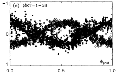
Figure 1: The active longitude structure on FK Com. Normalized magnitudes (ordinate) of FK Com for 1966–1990 plotted against the phase (abscissa). The phases have been determined using the ephemeris HJD 2439252.895 + 2.4002466 E. This figure has been taken from Jetsu et al. ([1993]).

After the discovery of the flip-flop phenomenon on FK Com it has been reported also on other active stars. Berdyugina & Tuominen ([1998]) studied the photometric observations of four RS CVn binaries and discovered that also these stars have permanent active longitudes that are alternatively active. In the case of II Peg Rodonò et al. ([2000]) later confirmed their results. Berdyugina, Pelt & Tuominen ([2002]) discovered flip-flops on young solar type star, LQ Hya. And a recent analysis of 120 years of sunspot data (Berdyugina & Usoskin [2003]) suggests that the Sun also has permanent active longitudes with associated flip-flops. On the Sun a flip-flop event occurs on average every 3.8 years on the northern and every 3.65 years on the southern hemisphere.

When the flip-flop phenomenon was discovered, it was not sure whether the phenomenon was caused by spot movement across the stellar disk or emergence of flux on the new active longitude. Korhonen et al. ([2001]) have shown, with Doppler images just before and after a flip-flop event on FK Com, that flip-flops are caused by changing the relative strengths of the spot groups at the two active longitudes without actual spot movement on the stellar surface.

All the stars for which the flip-flop phenomenon has been reported are listed in Table 1. Spectral type, rotation period and the relative differential rotation coefficient are given together with the flip-flop period (the length of the full cycle). The flip-flop phenomenon has so far been detected in many different kinds of stars: both binaries and single stars; young, main sequence and evolved alike. Usually, the flip-flop period is between 5 and 10 years, median being 7 years. The stars themselves usually have rotation periods $<3$ days (median 2.4 days). Anyhow, no clear correlation between the rotation period and the flip-flop period can be seen.

Apart from the stars mentioned in Table 1, there are also two other stars for which flip-flops have been reported. These stars are single giant HD199178 (Hackman [2004]) and RS CVn binary RT Lac (Lanza et al. [2002]). In these stars only very few events have been observed, so no information on the flip-flop cycle length can be obtained.

Table 1: Stars that show flip-flop phenomenon. In the Table the name of the star, spectral type and age, rotation period, flip-flop period and the relative differential rotation coefficient are given.

Name	Type	$P_{\rm rot}$	$P_{\rm ff}$	$\Delta\Omega/\Omega$
Sun	single, G2 V	27 d	71 yr	0.19
LQ Hya	single, K2 V, ZAMS	1.6 d	5.22 yr	0.0223
AB Dor	single, K0 V, ZAMS	0.5 d	5.54 yr	0.055
EK Dra	single, G1.5 V, ZAMS	2.6 d	44 yr	-
FK Com	single, G7 III	2.4 d	5.26 yr	0.0186
II Peg	RS CVn, K2 IV	6.7 d	9.37 yr	0.048
sigma Gem	RS CVn, K1 III	19.6 d	14.97 yr	$<0.004^{9}$
EI Eri	RS CVn, G5 IV	1.95 d	9.07 yr	-0.15 – -0.2010
HR 7275	RS CVn, K1 III-IV	2.3 d	17.57 yr	-

1)Berdyugina & Usoskin [2003] 2)Berdyugina et al. [2002] 3)Kővári et al. [2004] 4)Berdyugina & Järvinen [2005] 5)Collier Cameron & Donati [2002] 6)Korhonen et al. [2004] 7)Berdyugina & Tuominen [1998] 8)Weber [2004] 9)Kővári et al. [2001] 10)Washuettl [2004]

3 Modelling flip-flops

The model consists of a turbulent fluid in a spherical shell of inner radius $r_{\rm in}$ and outer radius $r_{\rm out}$.

We solve the induction equation

$${\partial\langle\vec{B}\rangle\over\partial t}={\rm curl}(\alpha_{q}\circ\langle\vec{B}\rangle-{\eta}_{\rm T}{\rm{curl}}\langle{\vec{B}}\rangle),$$ (1)

in spherical coordinates (${\rm r,\theta,\varphi}$) for an $\alpha^{2}\Omega$-dynamo. A solar type rotation law (see Fig. 2) in the corotating frame with the core

$$\Omega(r,\theta)={1\over 2}\Omega_{0}\left[1+{\rm erf}\left({r-r_{in}\over d_{1}}\right)\right](\Omega_{s}-\Omega_{c})$$ (2)

where $\Omega_{s}=\Omega_{eq}-a{\rm cos}^{2}\theta$ is used.

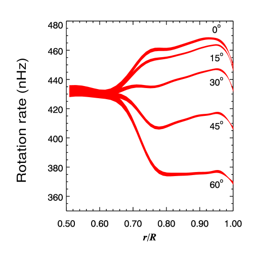
Figure 2: The solar rotation law.

Only the symmetric part

$$\alpha_{rr}=\alpha_{0}{\rm cos}\theta(1.-2{\rm cos}^{2}\theta)$$

$$\alpha_{\theta\theta}=\alpha_{0}{\rm cos}\theta(1.-2{\rm sin}^{2}\theta)$$

$$\alpha_{\varphi\varphi}=\alpha_{0}{\rm cos}\theta$$

$$\alpha_{r\theta}=\alpha_{\theta r}=2\alpha_{0}{\rm cos}^{2}\theta{\rm sin}\theta$$ (3)

of the $\alpha$-tensor is included. In order to saturate the dynamo we choose a local quenching of

$$\alpha_{q}={\alpha\over 1+\vec{B}^{2}/\vec{B}_{\rm eq}^{2}}$$

For $\alpha_{0}$ we choose a value slightly above the critical one for the dynamo threshold. The inner boundary is a perfect conductor and the outer boundary resembles a vacuum condition, by including an outer region up to 1.2 stellar radii into the computational grid with 10 times higher diffusivity. At the very outer part the pseudo vacuum condition is used. In order to see the influence of the thickness of the convection zone we have chosen $r_{\rm in}=0.7$ for a thin (results shown in Fig. 3) and $r_{\rm in}=0.4$ for a thick (Fig. 4) convection zone.

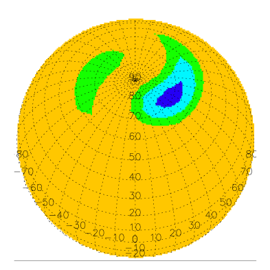
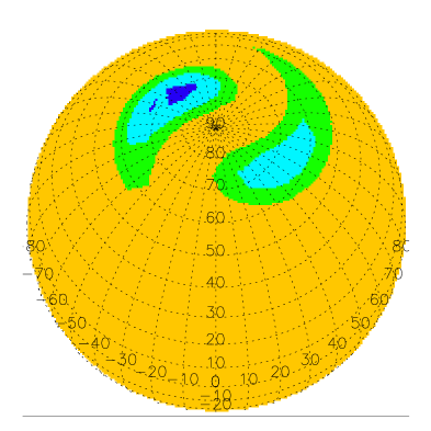
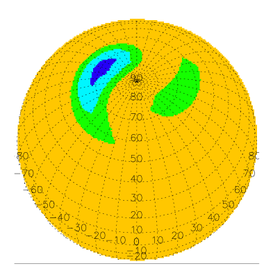
Figure 3: The magnetic pressure from the dominant radial component of the magnetic field on the stellar surface is shown at three different time steps for the thin layer model. We subtracted rotation and migration.

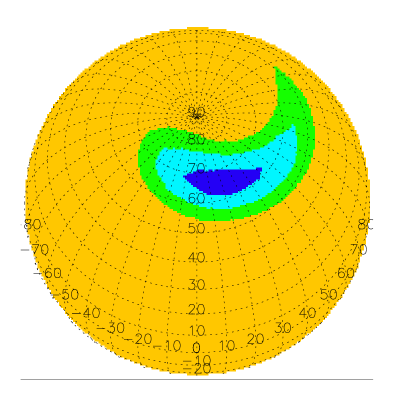
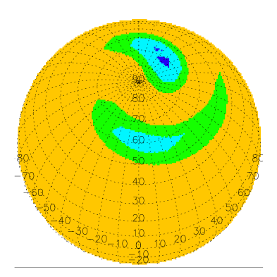
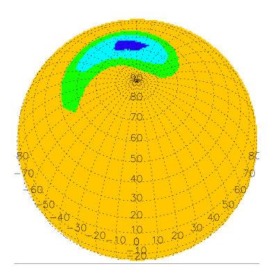
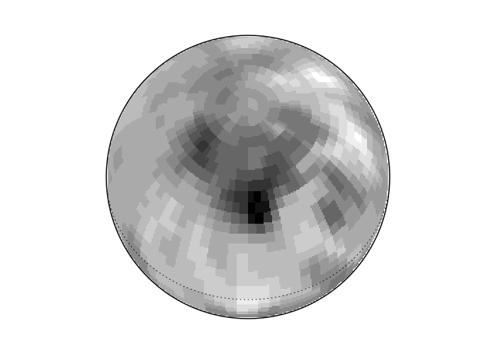
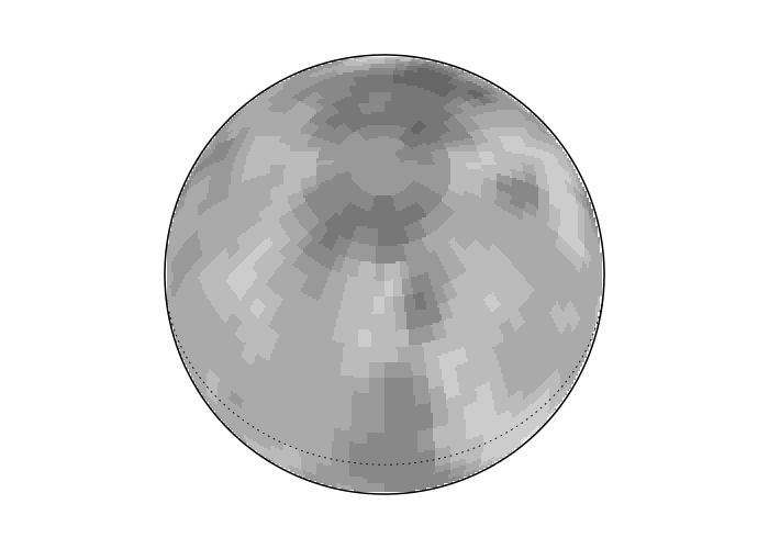
Figure 4: The upper panel is as in Fig. 3 but now for the thick convection zone model. The lower panel shows Doppler images of FK Com for June 1997 and January 1998 (from Korhonen et al. 2001). For the Doppler images the grey scale gives the temperature scale of 3600 K – 5700 K.

4 Results

With the parameter $\Omega_{0}$ we model the strength of the differential rotation. For $\Omega_{0}=1$ we have a solar rotation law with an oscillating axisymmetric dynamo solution. The case $\Omega_{0}=0$ is an $\alpha^{2}$-dynamo which gives a migrating non-axisymmetric dynamo because of the anisotropic $\alpha$ (cf. Rüdiger, Elstner & Ossendrijver [2003]). For 10% of the solar differential rotation we found similar excitation conditions for a drifting non-axisymmetric mode and an oscillating axisymmetric mode. Because of the chosen positive $\alpha$ in the northern hemisphere, we get a poleward migration of the oscillating mode. The drift of the non-axisymmetric mode is opposite to the rotation. Using a simple $\alpha$-quenching, given by Eq. 3, in 3D simulations we found coexisting solutions for both modes, showing a magnetic flip-flop phenomenon. We followed the solution in our simulation up to 100 diffusion times. There were no sign for it being only a temporary phenomenon. The temporal behaviour of the magnetic energy is shown in Fig. 5.

Figure 5: Energy density in $m=0$ and $m=1$ modes for the thick model normalized to equipartition. The time unit is the diffusion time of 30 years. Left: The whole simulation Right: Final time with higher resolution. Notice the weak oscillation of the energy in the $m=1$ mode synchronized with $m=0$ due to $\alpha$-quenching. The migration period in Table 2 is directly taken from the $m=1$ field.

For an assumed turbulent diffusivity of about $10^{12}{\rm cm}^{2}{\rm s}^{-1}$ we get a period of about 6 years for the thin and 9 years for the thick model. These values are mainly determined by the magnetic diffusivity and vary only weakly with the value for $\alpha$. The field strength saturates about the equipartition value. In Table 2 we present a choice of models in order to illustrate the parameter dependence of different solutions for an axisymmetric (first row), a non-axisymmetric (second row) and two flip-flop (thick and thin model; third and fourth row, respectively) solutions. Notice, that the axisymmetric solution appears already for $\Omega_{0}=0.1$ but with a higher $\alpha$ than is used for the thick convection zone flip-flop model (third row). This is probably due to the local quenching of the $m=1$ mode.

Table 2: Parameters for a sample of runs with the energy density in equipartition units E0 for the mode $m=0$ and E1 for $m=1$, respectively. P0 denotes the period of the oscillation in diffusion times (30 years) and P1 the migration period. The dynamo-number $C_{\alpha}={\alpha_{0}r_{star}\eta^{-1}}$ is used.

$r_{\rm in}$	$\Omega_{0}$	$C_{\alpha}$	E0	E1	P0	P1
0.4	0.1	20	1.4	$10^{-9}$	0.27
0.4	0.11	10	$10^{-6}$	0.1		0.23
0.4	0.12	10	0.06	0.06	0.3	0.2
0.7	0.11	21	0.1	0.4	0.23	0.46

For the thick convection zone we found models where the magnetic spots appear already at $50^{\circ}$ latitude and are migrating polewards during the cycle. In this case the opposite spot does not start to appear exactly $180^{\circ}$ away from the old spot. The distance can shrink down to $90^{\circ}$. It depends also on $\alpha$. For weakly over critical $\alpha$ we find nearly $180^{\circ}$ distance between old and new spot. In all models we found a counter-rotating migration of the magnetic pattern. The period was twice the flip-flop oscillation period for the thin layer and nearly equal to the flip-flop period for our thick layer model. This migration should be carefully considered in the future data analysis.

4.1 Comparison to FK Com

Korhonen et al. ([2004]) found that for FK Com the relative surface differential rotation ($\Delta\Omega/\Omega$) is about 10% of the solar value. This implies that the 10% scaling of the solar rotation law, that has been used in the model, is an appropriate first approximation for this star. In Fig. 4 the modeling results for the thick convection zone model are compared to the observed surface temperature distributions on FK Com for June 1997 and January 1998 (Korhonen et al. [2001]). In the calculations the spots appear at high latitudes. This is also consistent with the Doppler imaging results for FK Com, which show spots mainly at high latitudes, and basically never lower than latitude $45^{\circ}$. Also, the spot size looks reasonable and is in line with the observations.

5 Discussion

For the first time we found stable mixed mode solutions for weakly differential rotating stars. We could follow the cycle over 100 diffusion times. Moss ([2004]) presented a similar model with isotropic $\alpha$. Because there is no preferred m=1 mode in that case, it is probably not possible to have stable mixed mode solutions for a longer time. Also he did not find similar values for the magnetic energy in both modes. In contrary to our solution he got an asymmetric distribution of m=1 and $m=0$ modes with respect to the equator. We observed a similar exotic behaviour for highly over-critical $\alpha$. The assumptions for the model are somewhat uncertain. First, changing the diffusivity would change the period of the oscillating mode and therefore also the flip-flop period. The simple scaling of the solar rotation law may not be the best approximation for the stars showing flip-flops, also the simple $\alpha$-quenching non-linearity may not be adequate. Anyhow, the main properties remain for different quenching forms. Also, the simple diagonal form of the $\alpha$ tensor is not justified. Nevertheless, the results from our model are encouraging. The flip-flop phenomenon appears in a limited range of the strength of differential rotation. The thickness of the convection zone is not very important. To what extent a large scale meridional flow changes this behaviour has to be investigated.