Loitering universe models in light of the CMB

Abstract

Spatially flat loitering universe models have recently been shown to arise in the context of brane world scenarios. Such models allow more time for structure formation to take place at high redshifts, easing, e.g., the tension between the observed and predicted evolution of the quasar population with redshift. While having the desirable effect of boosting the growth of structures, we show that in such models the position of the first peak in the power spectrum of the cosmic microwave background anisotropies severely constrain the amount of loitering at high redshifts.

I Introduction

The last few years of intense observational developments have provided cosmology with a standard model: a universe with geometry described by the flat Robertson-Walker metric, with cold pressureless matter contributing roughly 1/3 and some form of negative pressure ‘dark energy’ contributing the remaining 2/3 of the critical energy density. The existence of the last component is motivated partly by the Hubble diagram from supernovae of type Ia (SNIa) riess ; perlmutter , partly from joint analysis of the cosmic microwave background (CMB) anisotropies and the large-scale distribution of matter, e.g. from the power spectrum of the galaxy distribution efstathiou ; tegmark . However, there are ways of describing the data which do not invoke a negative-pressure fluid, namely to postulate some modification of standard Einstein gravity on large scales. One way of realizing this is in the braneworld scenario, where our universe is taken to be a (3+1)-dimensional membrane (the brane) residing in a higher-dimensional space (the bulk), see shtanov for an overview. The standard model fields are confined to the brane, whereas gravity can propagate in the full space. The extra dimensions need not be small, and hence gravity can be modified on scales as large as the size of the present horizon $\sim c/H_{0}\sim 3000\;h^{-1}\,{\rm Mpc}$ (where $c$ is the speed of light, set equal to 1 in the remainder of this paper, and $H_{0}=100h\;{\rm km},\,{\rm s}^{-1}\,{\rm Mpc}^{-1}$ is the present value of the Hubble parameter.)

Loitering, i.e., a universe which undergoes a phase of very slow growth, can arise in closed universe models with a cosmological constant sahni2 . In the context of extra-dimensional models such phenomena can occur naturally in spatially flat geometries and may provide a solution to several problems. For instance, in brane gas cosmology(BGC) bgc , loitering may help to solve the horizon problem and the brane problem of BGC brand . Recently, the possibility of a loitering phase has been pointed out by Sahni and Shtanov sahni in the context of other braneworld models, where the geometry on our brane is spatially flat. Such a phase has desirable consequences, since it allows more time for structure formation feldman and astrophysical processes, alleviating some of the tension between the concordance $\Lambda{\rm CDM}$ model and the observations of quasars with redshifts $z\sim 6$ richards ; haiman and the indications from WMAP of early reionization wmap . The loitering phase is proposed to occur at high redshifts $z\sim 20$, and the behavior of these loitering models at moderate redshifts is similar to the $\Lambda{\rm CDM}$ model, thus making it possible to satisfy constraints from e.g. SNIa. However, as we will show in this paper, the position of the first peak of the power spectrum of the CMB anisotropies places a very robust constraint on the high-redshift behavior of all models.

The structure of this Brief Report is as follows. We start out by introducing the loitering braneworld models in section II, and confront them with data in section III. In section IV we look at constraints on loitering in general from the CMB peak positions. We summarize and conclude in section V.

II The loitering brane world model

The braneworld models considered in sahni are defined by the action

$$\mbox{$$}S = M^{3}\Big{[}\int_{\rm bulk}d^{5}x\sqrt{-g}\Big{(}\mathcal{R}-2\Lambda_{b}\Big{)}-2\int_{\rm brane}d^{4}x\sqrt{-g^{(4)}}K\Big{]}$$ (1)

$$+m^{2}\int_{\rm brane}d^{4}x\sqrt{-g^{(4)}}\Big{(}\mathcal{R}^{(4)}-2{\sigma\over m^{2}}\Big{)}$$

$$+\int_{\rm brane}d^{4}x\sqrt{-g^{(4)}}\mathcal{L},$$

where $M$ and $m$ are the five and four dimensional Planck masses, $\Lambda_{b}$ the bulk cosmological constant and $\sigma$ the brane tension. The Friedmann equation of the loitering brane world model is sahni :

$$\mbox{$$}\Big{(}{H(z)\over H_{0}}\Big{)}^{2} = \Omega_{\textrm{\footnotesize m}}(1+z)^{3}+\Omega_{\footnotesize\sigma}+2\Omega_{\footnotesize\ell}-2\sqrt{\Omega_{\footnotesize\ell}}\Big{[}\Omega_{\footnotesize\sigma}+\Omega_{\footnotesize\ell}$$ (2)

$$+\Omega_{\textrm{\footnotesize m}}(1+z)^{3}+\Omega_{\footnotesize\Lambda_{\textrm{b}}}+\Omega_{\textrm{\footnotesize C}}(1+z)^{4}\Big{]}^{1/2}$$

where

$$\Omega_{\textrm{\footnotesize m}}={\rho_{\rm m}^{0}\over 3m^{2}H_{0}^{2}},\ \Omega_{\footnotesize\sigma}={\sigma\over 3m^{2}H_{0}2^{2}},\ \Omega_{\footnotesize\ell}={1\over l^{2}H_{0}^{2}}$$

$$\Omega_{\footnotesize\Lambda_{\textrm{b}}}=-{\Lambda_{b}\over 6H_{0}^{2}},\ \Omega_{\textrm{\footnotesize C}}=-{C\over a_{0}^{4}H_{0}^{2}}.$$ (3)

The $\Omega_{\textrm{\footnotesize C}}$ term is the dark radiation energy density arising from the brane-bulk interaction. The condition for a spatially flat universe is

$$\mbox{$$}\Omega_{\footnotesize\sigma}=1-\Omega_{\textrm{\footnotesize m}}+2\sqrt{\Omega_{\footnotesize\ell}}\sqrt{1+\Omega_{\footnotesize\Lambda_{\textrm{b}}}+\Omega_{\textrm{\footnotesize C}}}.$$ (4)

Late time acceleration occurs at the critical length scale corresponding to the present horizon scale, i.e., $l=2m^{2}/M^{3}\sim H_{0}^{-1}$, which sets $\Omega_{\footnotesize\ell}\sim{\cal O}(1)$. Since $\Omega_{\footnotesize\Lambda_{\textrm{b}}}$ corresponds to the five-dimensional bulk cosmological constant, it can naturally have a much larger value than the other parameters that correspond to quantities on the brane, $\Omega_{\footnotesize\Lambda_{\textrm{b}}}\gg\Omega_{\textrm{\footnotesize m}},\ \Omega_{\textrm{\footnotesize C}},\ \Omega_{\footnotesize\ell}$. Hence, at high redshifts, $z\;\raise 1.29167pt\hbox{$>$\kern-7.5pt\raise-4.73611pt\hbox{$\sim$}}\;10$, at which loitering occurs, we can well approximate Eq. (2) by:

$$\mbox{$$}\Big{(}{H(z)\over H_{0}}\Big{)}^{2} \approx \Omega_{\textrm{\footnotesize m}}(1+z)^{3}+2\sqrt{\Omega_{\footnotesize\ell}\Omega_{\footnotesize\Lambda_{\textrm{b}}}}$$ (5)

$$-2\sqrt{\Omega_{\footnotesize\ell}}\Big{(}\Omega_{\footnotesize\Lambda_{\textrm{b}}}+\Omega_{\textrm{\footnotesize C}}(1+z)^{4}\Big{)}^{1/2}.$$

Note that this is somewhat different what was considered in sahni where they also drop the $\Omega_{\footnotesize\Lambda_{\textrm{b}}}$ term inside the last square root. However, using the example parameter values given in sahni , one sees that this is not well justified.

As discussed in sahni , the Friedmann equation can exhibit different behavior depending on the values of the parameters. Here we are interested in loitering behavior with respect to the $\Lambda$CDM model and hence instead of $H(z)$, we consider $X(z)\equiv H/H_{\Lambda{\rm CDM}}$. This function has a well defined minimum for parameter values for which the interpretation of $H(z)$ is not as straightforward (see Fig. 1 in sahni ).

We can now unambiguously define the loitering redshift as $X^{\prime}(z_{\rm loit})=0$. In the high redshift approximation, one finds that

$$\mbox{$$}1+z_{\rm loit}=\Big{(}3{\Omega_{\footnotesize\Lambda_{\textrm{b}}}\over\Omega_{\textrm{\footnotesize C}}}\Big{)}^{1/4}.$$ (6)

Positivity at this minimum point, $H^{2}(z_{\rm loit})>0$, gives us a condition on $\Omega_{\footnotesize\Lambda_{\textrm{b}}}$:

$$\mbox{$$}\Omega_{\footnotesize\Lambda_{\textrm{b}}}>{2^{4}\over 3^{3}}{\Omega_{\footnotesize\ell}^{2}\Omega_{\textrm{\footnotesize C}}^{3}\over\Omega_{\textrm{\footnotesize m}}^{4}}.$$ (7)

Within the high loitering redshift approximation, it is then clear that for a given loitering redshift, $z_{\rm loit}$, $\Omega_{\textrm{\footnotesize C}}$ is constrained by

$$\mbox{$$}3{\Omega_{\footnotesize\Lambda_{\textrm{b}}}\over(1+z_{\rm loit})^{4}}<\Omega_{\textrm{\footnotesize C}}<({3^{3}\Omega_{\textrm{\footnotesize m}}^{4}\over 2^{4}\Omega_{\footnotesize\ell}^{2}}\Omega_{\footnotesize\Lambda_{\textrm{b}}})^{1/3},$$ (8)

indicating that both $\Omega_{\textrm{\footnotesize C}}$ and $\Omega_{\footnotesize\Lambda_{\textrm{b}}}$ have a maximum value for a given $z_{\rm loit}$.

III Constraints on braneworld loitering

The CMB shift parameter determines the shift of the peaks in the CMB power spectrum when cosmological parameters are varied bond ; melchiorri ; odman . It is given by

$${{\cal R}}=\sqrt{\Omega_{\rm m}}H_{0}r(z_{\rm dec}),$$ (9)

where $r(z)=\int_{0}^{z}dz/H(z)$ is the comoving distance in a flat universe, and $z_{\rm dec}$ is the redshift at decoupling. This expression is derived in the $\Lambda{\rm CDM}$ model, and depends on the ratio between the sound horizon at decoupling and the angular diameter distance to $z_{\rm dec}$. We can apply it straightforwardly in our case also, since the only way equation (9) could be radically changed is if the sound horizon were to change significantly in the brane world models conidered here, and we have checked that this is not the case. Observationally, from WMAP we have $z_{\rm dec}=1088^{+1}_{-2}$, and ${{\cal R}}_{\rm obs}=1.716\pm 0.062$ wmap .

The WMAP constraint on ${{\cal R}}$ places severe constraints on loitering models. We have run a grid of models, fixing $\Omega_{\rm m}=0.3$, $\Omega_{\rm l}=3.0$, and allowing $\Omega_{\Lambda_{\rm b}}$ and $\Omega_{\rm C}$ to vary. We compute ${{\cal R}}$ from Eq. (9), and compute $\chi^{2}=({{\cal R}}-{{\cal R}}_{\rm obs})^{2}/\sigma_{{\cal R}}^{2}$, where $\sigma_{{\cal R}}=0.062$. The resulting contours are shown in Fig. 1. They effectively rule out any significant amount of loitering.

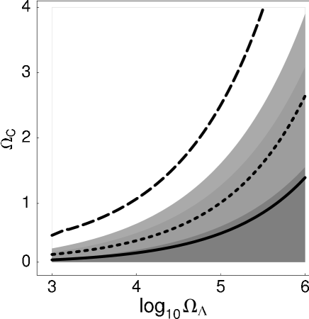
Figure 1: Confidence contours (68(darkest), 95 and 99(lightest) %) imposed by the CMB shift parameter on the parameters $\Omega_{\Lambda_{\rm b}}$ and $\Omega_{\rm C}$. Also shown are lines of constant increase in age at $z=6$ compared with the $\Lambda{\rm CDM}$ model: $\Delta t=0.05$ (solid), $0.1$ (dotted), $0.3$ (dashed) Gyr.

For example, picking a model along the 68 % contour, one finds that deviations from the standard $\Lambda{\rm CDM}$ behavior are tiny. In figure 1 we have also plotted contours of constant increase in age at $z=6$ for the loitering model compared with the $\Lambda{\rm CDM}$ model, in units of Gyr. The age of the $\Lambda{\rm CDM}$ model at $z=6$ is $0.92\;{\rm Gyr}$ for $\Omega_{\rm m}=0.3$, $h=0.7$. Only a modest increase in age is allowed, a change of $0.3\;{\rm Gyr}$ being ruled out at more than 99% confidence.

One can also quantify the amount of loitering allowed by considering how structures grow in the braneworld model considered here, compared to the $\Lambda$CDM model. The linear growth factor, $D$, is given by

$$\mbox{$$}\ddot{D}+2H\dot{D}-\frac{3}{2}{\Omega_{\textrm{\footnotesize m}}\over a^{3}}D=0$$ (10)

and it is easy to see that in the Einstein de Sitter-case, a simple growing solution exists, $D\sim a$. We have calculated how the linear growth factor evolves in the braneworld model for different values of the parameters and compared it to the value in the $\Lambda$CDM model. The results are shown in Fig. 2 for $z=6$. As a reference, for $\Omega_{\textrm{\footnotesize C}}=8.0$, $\Omega_{\footnotesize\Lambda_{\textrm{b}}}=4.5\times 10^{5}$ considered in sahni (and clearly ruled out by the shift parameter) for which $H(z)$ has a clear loitering phase at $z\sim 20$, one finds that $D/D_{\Lambda CDM}(z=6)\approx 42$.

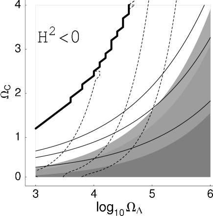
Figure 2: The loitering redshift $z_{\rm loit}=10,\,15,\,20$ (dashed lines, left to right), relative linear growth factor at $z=6$, $D/D_{\Lambda}=1.5,\,2.0,\,2.5$ (solid lines, bottom to top) and the shift parameter confidence regions (in gray) for different values of $(\Omega_{\Lambda_{\rm b}},\Omega_{\rm C})$. Also shown is the excluded region where $H(z_{\rm loit})^{2}<0$.

From the figure one sees that within the $99\%$ region, with $z_{\rm loit}=20$, the linear growth factor can only be about twice the value of that in the $\Lambda$CDM model.

IV Loitering in general

The constraints found in the previous section are easily understood to arise from the fact that if the Hubble parameter is decreased compared to $\Lambda{\rm CDM}$ at high redshifts, the comoving distance to the last scattering surface is increased. Thus, the conclusion that loitering is effectively constrained by the CMB shift parameter is not specific to the braneworld model, and can be generalized as shown in the following.

What makes a loitering phase attractive, is the fact that $H(z)$ is less than the Hubble parameter in $\Lambda{\rm CDM}$ during loitering, so that the universe can spend more time at high redshifts. In order to quantify this effect, we model the loitering phase by having a Hubble parameter that reduced by a factor $0<\alpha<1$ compared with its $\Lambda{\rm CDM}$ value in an interval $z_{1}<z<z_{2}$, where $z_{2}<z_{\rm dec}$. Then the time the universe spends between $z_{1}$ and $z_{2}$ is increased by a factor $1/\alpha$, since $t(z_{1})-t(z_{2})=\int_{z_{1}}^{z_{2}}dz/((1+z)H(z))$. The corresponding change in the comoving distance to the last scattering surface compared with the $\Lambda{\rm CDM}$ model is $(1/\alpha-1)\int_{z_{1}}^{z_{2}}dz/H_{\Lambda{\rm CDM}}(z)$, and so the change in the shift parameter is

$$\Delta{{\cal R}}=\sqrt{\Omega_{\rm m}}H_{0}\left(\frac{1}{\alpha}-1\right)\int_{z_{1}}^{z_{2}}\frac{dz}{\sqrt{\Omega_{\rm m}(1+z)^{3}+(1-\Omega_{\rm m})}}.$$ (11)

In Fig. 3, where we show the result of fitting the parameters $\alpha$ and $\beta\equiv z_{2}-z_{1}$ to the CMB shift parameter. The upper panel shows the likelihood contours for a dip in the Hubble parameter which starts at a redshift of 10, and in the lower panel the dip starts at a redshift of 500. As can be seen from the figure, one can have either a substantial dip ($\alpha\rightarrow 0$) over a very small redshift interval ($\beta\approx 0$), or a small dip ($\alpha\approx 1$) over a large redshift interval ($\beta>>1$). In both cases, the age of the Universe at $z=6$ increases marginally.

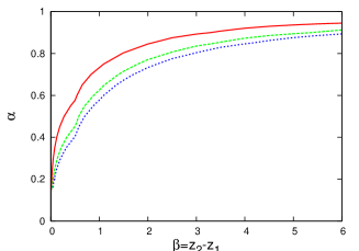
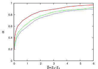
Figure 3: (Colour online only) 68, 95 and 99 percent confidence contours imposed by the CMB shift parameter on the parameters $\alpha$ and $\beta$ for $z_{1}=10$ (upper panel) and $z_{1}=500$ (lower panel). The $\Lambda$CDM model corresponds to the lines $\alpha=1$ or $\beta=0$

In fact, we can be even more general and consider that the Hubble parameter is some $H(z)$ for $z_{1}<z<z_{2}$, and equal to the Hubble parameter of $\Lambda{\rm CDM}$ at all other redshifts. Assuming $z_{1}<z_{2}<z_{\rm dec}$, the change in the age compared to the pure $\Lambda{\rm CDM}$ model is

$$\mbox{$$}\Delta t(z_{1})=\int_{z_{1}}^{z_{2}}{dz\over 1+z}\Big{(}{1\over H(z)}-{1\over H_{\Lambda{\rm CDM}}(z)}.\Big{)}$$ (12)

Since $1/(1+z)\leq 1/(1+z_{1})$, we have

$$\mbox{$$}\Delta t(z_{1})<\frac{1}{z_{1}+1}\Omega_{\rm m}^{-1/2}H_{0}^{-1}\Delta{{\cal R}}.$$ (13)

For example, for $z_{1}=6$, with $h=0.7,\ \Omega_{\rm m}=0.3,\ \Delta{\cal R}=0.062$, this gives the upper limit

$$\mbox{$$}\Delta t(z=6)<0.22\;{\rm Gyr}.$$ (14)

In terms of the linear growth factor, general constraints are not as straightforward to derive as now the exact features of the loitering phase play a crucial role. The linear growth rate in terms of the scale factor with $H=XH_{\Lambda CDM}$ is

$$\mbox{$$}D^{\prime\prime}+\Big{(}{3\over a}+{H_{\Lambda CDM}^{\prime}\over H_{\Lambda CDM}}+{X^{\prime}\over X}\Big{)}D^{\prime}-\frac{3}{2}{H_{0}^{2}\over H_{\Lambda CDM}^{2}}{\Omega_{\textrm{\footnotesize m}}\over a^{5}}{1\over X^{2}}D=0,$$ (15)

where ${}^{\prime}\equiv d/da$. Since loitering occurs at high redshifts, we can well approximate $H^{2}_{\Lambda CDM}\approx H^{2}_{EdS}=H_{0}^{2}\Omega_{\textrm{\footnotesize m}}/a^{3}$. Approximating the loitering phase by $X(z)\approx X_{0}$ one finds that during this phase, $D\sim a^{\beta}$, with $\beta=(-1+\sqrt{24/X_{0}^{2}+1})/4$. For $X_{0}<1$, i.e. when the universe is loitering, $\beta$ is larger than one indicating faster growth than in the $\Lambda$CDM (EdS) model. Quantifying the effect requires detailed knowledge about the loitering phase, making the age constraint, Eq. (14), a more robust constraint on any flat loitering model.

V Conclusions

We have considered flat loitering universe models, both in the specific context of braneworld scenarios, and in general. While increasing the time the universe spends at high redshifts and enhancing the linear growth factor might have desirable consequences for, e.g., modeling of the quasar population, modifications of the behavior of the Hubble parameter at high redshifts lead to changing the size of the sound horizon at recombination. As this quantity is well measured by the position of the peaks in the CMB angular power spectrum, only a modest change is possible. Hence, a substantial increase in the age or linear growth factor at, say, $z=6$ are not allowed. Only a modest increase in both quantities is possible, indicating that if a much older universe (or enhanced growth factor)is needed to accommodate observations, another new cosmological scenario is required.

- (1) A. G. Riess et al., Astron. J. 116 (1998) 1009
- (2) S. Perlmutter et al., Astrophys. J. 517 (1999) 565
- (3) G. Efstathiou et al., MNRAS 330 (2002) L29
- (4) M. Tegmark et al., Phys. Rev. D 69 (2003) 103501
- (5) V. Sahni and Y. Shtanov, JCAP 0311 (2003) 014
- (6) V. Sahni, H. Feldman, and A. Stebbins, Astrophys. J. 385 (1992) 1
- (7) S. Alexander, R. Brandenberger, D. Easson, Phys. Rev. D 62 (2000) 103509
- (8) R. Brandenberger, D. Easson, D. Kimberly, Nuc. Phys. B, 623 (2002) 421.
- (9) V. Sahni and Y. Shtanov, 2004, preprint (astro-ph/0410221)
- (10) H. Feldman, A. Evrard, Int. J. Mod. Phys. D 2 (1993) 113, astro-ph/9212002
- (11) G. T. Richards et al., Astron. J. (2004) 127 1305
- (12) Z. Haiman and E. Quataert, astro-ph/0403225 Astrophys. J. Suppl. 148, 175 (2003)
- (13) D. N. Spergel et al., Ap.J.S. 148 (2003) 175
- (14) J. R. Bond, G. Efstathiou and M. Tegmark, MNRAS 291 (1997) L33
- (15) A. Melchiorri, L. Mersini, C. J. Ödman and M. Trodden, Phys. Rev. D 68 (2003) 043509
- (16) C. J. Ödman, A. Melchiorri, M. P. Hobson and A. N. Lasenby, Phys. Rev. D 67 (2003) 083511