Relic Gravitational Waves in the Accelerating Universe

Abstract

Observations have recently indicated that the Universe at the present stage is in an accelerating expansion, a process that has great implications. We evaluate the spectrum of relic gravitational waves in the current accelerating Universe and find that there are new features appearing in the resulting spectrum as compared to the decelerating models. In the low frequency range the peak of spectrum is now located at a frequency $\nu_{E}\simeq(\frac{\Omega_{m}}{\Omega_{\Lambda}})^{1/3}\nu_{H}$, where $\nu_{H}$ is the Hubble frequency, and there appears a new segment of spectrum between $\nu_{E}$ and $\nu_{H}$. In all other intervals of frequencies $\geq\nu_{H}$, the spectral amplitude acquires an extra factor $\frac{\Omega_{m}}{\Omega_{\Lambda}}$, due to the current acceleration, otherwise the shape of spectrum is similar to that in the decelerating models. The recent WMAP result of CMB anisotropies is used to normalize the amplitude for gravitational waves. The slope of the power spectrum depends sensitively on the scale factor $a(\tau)\propto|\tau|^{1+\beta}$ during the inflationary stage with $\beta=-2$ for the exact de Sitter space. With the increasing of $\beta$, the resulting spectrum is tilted to be flatter with more power on high frequencies, and the sensitivity of the second science run of the LIGO detectors puts a restriction on the parameter $\beta\leq-1.8$. We also give a numerical solution which confirms these features.

PACS numbers: 98.80.-k, 98.80.Es, 04.30.-w, 04.62+v,

Key words: gravitational waves, accelerating universe, dark energy

e-mail: yzh@ustc.edu.cn

1. Introduction.

The inflationary expansion of the early Universe can create a stochastic background of relic gravitational waves, which is important in cosmology and has been extensively studied in the past [1] [2] [3] [4] [5]. The spectrum of relic gravitational waves, as is to be observed today, depends not only on the details of the early stage of inflationary expansion, but also on the expansion behavior of the subsequent stages, including the current one. The calculations of spectrum so far [6] [7] [8] [9] [10] [11] have been done for the case that the current stage is in a decelerating expansion. The resulting spectrum has been put among the candidate list of sources for the gravitational wave detectors either in operation [12][13], or under construction [14] [15]. The astronomical observations on SN Ia [16] [17] indicate that the Universe is currently under accelerating expansion, which may be driven by the cosmic dark energy ($\Omega_{\Lambda}\sim 0.7$) plus the dark matter ($\Omega_{m}\sim 0.3$) [18]. This is further supported by the recent WMAP results on CMB anisotropies [19] with $\Omega=1$. By the wave equation, the evolution of relic gravitational waves depends on the expanding spacetime background, and the wave amplitudes depend on whether the wave lengths are inside or outside the Hubble radius. The Universe under accelerating expansion has a Hubble radius as a function of time that differs from that in the conventional models of decelerating expansion. Therefore, one can expect that, if an earlier matter-dominated stage of decelerating expansion is followed by the current accelerating expansion, the outcome for the spectrum of relic gravitational waves will be altered.

In this paper we study the impact of the current accelerating expansion on the relic gravitational waves. We will first sketch, as a setup, the well-known formulations of the gravitational waves in an expanding spacetime [20], and give the explicit scale factor $a(\tau)$ for a sequence of successive expanding epochs, including the current epoch of accelerating expansion. We then evaluate the power spectrum of relic gravitational waves and find that the current accelerating expansion does change the spectrum, including its shape and amplitude. Throughout the paper we shall work with units with $c=\hbar=1$, otherwise it will be pointed out. We also use notations similar to that of Grishchuk [8] for convenience for comparison.

2. The Gravitational Wave Equation.

Incorporating the perturbations to the spatially flat Robertson-Walker space-time, the metric is

$$ds^{2}=a^{2}(\tau)[d\tau^{2}-(\delta_{ij}+h_{ij})dx^{i}dx^{j}],$$ (1)

where where $\tau$ is the conformal time, the perturbations of spacetime $h_{ij}$ is a $3\times 3$ symmetric matrix containing generally the scalar, vector, and tensor parts. The gravitational wave field is the tensorial portion of $h_{ij}$, which is transverse-traceless

$$\partial_{i}h^{ij}=0,\,\,\,\,\delta^{ij}h_{ij}=0.$$ (2)

We are interested only in the creation of the relic gravitational waves by the expanding spacetime background, the perturbed matter source is therefore not taken into account. Moreover, as the relic gravitational waves are very weak, in the sense that $h_{ij}\ll 1$, so one need just study the linearized field equation:

$$\partial_{\mu}(\sqrt{-g}\partial^{\mu}h_{ij}({\bf{x}},\tau))=0.$$ (3)

In quantum theory of gravitational waves, the field $h_{ij}$ is a field operator, which is written as a sum of the plane wave Fourier modes

$$h_{ij}({\bf{x}},\tau)\frac{\sqrt{16\pi}l_{Pl}}{(2\pi)^{\frac{3}{2}}}\sum_{\lambda=1}^{2}\int_{-\infty}^{\infty}d^{3}{\bf k}\epsilon^{(\lambda)}_{ij}({\bf k})\frac{1}{\sqrt{2k}}[a_{k}^{(\lambda)}h^{(\lambda)}_{k}(\tau)e^{i\bf k\cdot x}+a_{k}^{\dagger(\lambda)}h^{(\lambda)*}_{k}(\tau)e^{-i\bf k\cdot x}],$$ (4)

where $l_{Pl}=\sqrt{G}$ is the Planck’s length, the two polarizations $\epsilon^{(\lambda)}_{ij}(\bf k)$, $\lambda=1,2$, are symmetric and transverse-traceless $k^{i}\epsilon^{(\lambda)}_{ij}({\bf k})=0$, $\delta^{ij}\epsilon^{(\lambda)}_{ij}({\bf k})=0$, and satisfy the conditions $\epsilon^{(\lambda)ij}({\bf k})\epsilon^{(\lambda^{\prime})}_{ij}({\bf k})=2\delta_{\lambda\lambda^{\prime}}$, and $\epsilon^{(\lambda)}_{ij}({\bf-k})=\epsilon^{(\lambda)}_{ij}({\bf k})$, the creation and annihilation operators satisfy $[a_{\bf k}^{(\lambda)},a_{\bf k^{\prime}}^{\dagger(\lambda^{\prime})}]=\delta_{\lambda\lambda^{\prime}}\delta^{3}({\bf k}-{\bf k^{\prime}})$, and the initial vacuum state is defined as

$$a_{\bf k}^{(\lambda)}\mid 0>=0$$ (5)

for each $\bf k$ and $\lambda$. As a matter of fact, this definition depends on the choice of the mode function $h^{(\lambda)}_{k}(\tau)$; different $h^{(\lambda)}_{k}(\tau)$ define different vacuum states, a point that will be further explained later. In the vacuum state the energy density of gravitational waves $t_{00}=\frac{1}{32\pi G}h_{ij,\,0}h^{ij}_{\,\,,\,0}$ gives the zero-point energy

$$<0|\int t_{00}d^{3}{\bf x}|0>=\frac{1}{2}\hbar\int^{\infty}_{-\infty}d^{3}{\bf k}\sum_{\lambda=1}^{2}\omega_{k}<0|a^{(\lambda)}_{\bf k}a^{(\lambda)\dagger}_{\bf k}|0>.$$

For a fixed wave number $\bf k$ and a fixed polarization state $\lambda$, the Eq.(3) reduces to the second-order ordinary differential equation [20]

$$h_{k}^{(\lambda)^{\prime\prime}}(\tau)+2\frac{a^{\prime}}{a}h_{k}^{(\lambda)^{\prime}}(\tau)+k^{2}h^{(\lambda)}_{k}=0,$$ (6)

where the prime denotes $d/d\tau$. Since the equation of $h_{\bf k}^{(\lambda)}(\tau)$ for each polarization is the same, we denote $h_{\bf k}^{(\lambda)}(\tau)$ by $h_{\bf k}(\tau)$. One rescales the field $h_{\bf k}(\tau)$ as

$$h_{\bf k}(\tau)\frac{\mu_{\bf k}(\tau)}{a(\tau)},$$ (7)

and the equation for $\mu_{\bf k}$ is

$$\mu_{k}^{\prime\prime}+(k^{2}-\frac{a^{\prime\prime}}{a})\mu_{k}=0.$$ (8)

This equation can be regarded as the equation for one-dimensional oscillator in a given effective potential barrier $a^{\prime\prime}/a$. For a given spacetime background with a generic power-law form of the scale factor

$$a(\tau)\propto\tau^{\alpha},$$ (9)

where $\alpha$ is a real number, positive or negative, the general solution is a linear combination of the Hankel’s functions:

$$\mu_{k}(\tau)A_{k}\sqrt{k\tau}H^{(1)}_{(\alpha-\frac{1}{2})}(k\tau)+B_{k}\sqrt{k\tau}H^{(2)}_{(\alpha-\frac{1}{2})}(k\tau).$$ (10)

Given a model of the expansion of Universe, consisting of a sequence of successive $a(\tau)$ as in Eq.(9) with different $\alpha$, one can construct an exact solution $\mu_{k}(\tau)$ by matching its values and its derivatives at the joining points. One may may also numerically solve Eq.(6) and give the corresponding power spectrum as we will present later in the paper. The vacuum state $|0>$, determined by the mode function $h_{k}(\tau)$, is therefore fixed by a choice of coefficients $A_{k}$ and $B_{k}$. In the limit $k\rightarrow\infty$, or $\tau\rightarrow\pm\infty$,

$$\sqrt{k\tau}H^{(1)}_{(\alpha-\frac{1}{2})}(k\tau)\rightarrow\sqrt{\frac{2}{\pi}}i^{-\alpha}e^{-ik\tau},$$

$$\sqrt{k\tau}H^{(2)}_{(\alpha-\frac{1}{2})}(k\tau)\rightarrow\sqrt{\frac{2}{\pi}}i^{\alpha}e^{ik\tau},$$

approaching the positive and negative frequency modes, respectively. For instance, if we choose $B_{k}=0$, then in the limit $k\rightarrow\infty$, or $\tau\rightarrow\pm\infty$,

$$h_{\bf k}(\tau)\propto e^{-ik\tau},$$

giving the positive frequency mode. This choice yields the so-called adiabatic vacuum [21] through (4) and (5). The amplitude of the power spectrum of the gravitational waves depends only on the initial value of $|h_{\bf k}(\tau)|$ at the horizon-crossing.

The following two limiting cases are useful for an approximate evaluation of the spectrum. Outside the barrier $k^{2}\gg\frac{a^{\prime\prime}}{a}$ (equivalent to $k\gg\frac{a^{\prime}}{a}$) the gravitational wave field reduces to

$$h_{k}(\tau)\rightarrow A_{k}\frac{e^{ik\tau}}{a(\tau)}+B_{k}\frac{e^{-ik\tau}}{a(\tau)},$$ (11)

having a decreasing amplitude

$$h_{k}(\tau)\propto 1/a(\tau).$$ (12)

Inside the barrier $k^{2}\ll\frac{a^{\prime\prime}}{a}$ (equivalent to $k\ll\frac{a^{\prime}}{a}$) the gravitational wave field

$$h_{k}(\tau)\rightarrow C_{k}+D_{k}\int^{\tau}\frac{d\tau^{\prime}}{a^{2}(\tau^{\prime})}.$$ (13)

The second term $D\int^{\tau}\frac{d\tau^{\prime}}{a^{2}(\tau^{\prime})}$ is small for the models that we shall study in the following, so the long wave-length limit of $h_{k}$ is simply a constant:

$$h_{k}(\tau)=C_{k}.$$ (14)

Thus, as a function of $\tau$, $h_{k}(\tau)$ has simple approximate behaviors in the two limiting cases, and we will use these to estimate the spectrum at present stage.

3. Epochs of Expanding Universe

The history of overall expansion of the Universe can be modelled as the following sequence of successive epochs of power-law expansion.

The initial stage (inflationary)

$$a(\tau)=l_{0}\mid{\tau}\mid^{1+\beta},\,\,\,\,\,-\infty<\tau\leq\tau_{1},$$ (15)

where $1+\beta<0$, and $\tau_{1}<0$. The special case of $\beta=-2$ is the de Sitter expansion.

The z-stage

$$a(\tau)=a_{z}(\tau-\tau_{p})^{1+\beta_{s}},\,\,\,\,\,\tau_{1}\leq\tau\leq\tau_{s},$$ (16)

where $\beta_{s}+1>0$. Towards the end of inflation, during the reheating, the equation of state of energy in the Universe can be quite complicated and is rather model-dependent [22]. So this z-stage is introduced to allow a general reheating epoch, as has been advocated by Grishchuk [8].

The radiation-dominated stage

$$a(\tau)=a_{e}(\tau-\tau_{e}),\,\,\,\,\,\tau_{s}\leq\tau\leq\tau_{2}.$$ (17)

The matter-dominated stage

$$a(\tau)=a_{m}(\tau-\tau_{m})^{2},\,\,\,\,\,\tau_{2}\leq\tau\leq\tau_{E},$$ (18)

where $\tau_{E}$ is the time when the dark energy density $\rho_{\Lambda}$ is equal to the matter energy density $\rho_{m}$. Before the discovery of the accelerating expansion of the Universe, the current expansion was usually taken to be in this matter-dominated stage, which is a decelerating one. Now, following the matter-dominated stage, we add an epoch of accelerating stage . The value of the redshift $z_{E}$ at the time $\tau_{E}$ is given by $(1+z_{E})=a(\tau_{H})/a(\tau_{E})$, where $\tau_{H}$ is the present time. Since $\rho_{\Lambda}$ is constant and $\rho_{m}(\tau)\propto a^{-3}(\tau)$, one has

$$1=\frac{\rho_{\Lambda}}{\rho_{m}(\tau_{E})}=\frac{\rho_{\Lambda}}{\rho_{m}(\tau_{H})(1+z_{E})^{3}}.$$

If we take the current values $\Omega_{\Lambda}\sim 0.7$ and $\Omega_{m}\sim 0.3$, then it follows that

$$1+z_{E}=(\frac{\Omega_{\Lambda}}{\Omega_{m}})^{1/3}\sim 1.33.$$

The accelerating stage (up to the present)

$$a(\tau)=l_{H}\mid\tau-\tau_{a}\mid^{-1},\,\,\,\,\,\tau_{E}\leq\tau\leq\tau_{H}.$$ (19)

This stage describes the accelerating expansion of the Universe, which is the new feature in our model and will induce some modifications to the spectrum of the relic gravitational waves. It should be mentioned that the actual scale factor function $a(\tau)$ differs from Eq.(19), since the matter component exists in the current Universe. However, the dark energy is dominant, so (19) is an approximation to the current expansion behavior.

Given $a(\tau)$ for the various epochs, the derivative $a^{\prime}=da/d\tau$ and the ratio $a^{\prime}/a$ follow immediately. Except for the $\beta_{s}$ that is imposed upon as the model parameter, there are ten constants in the above expressions of $a(\tau)$. By the continuity conditions of $a(\tau)$ and $a(\tau)^{\prime}$ at the four given joining points $\tau_{1}$, $\tau_{s}$, $\tau_{2}$, and $\tau_{E}$, one can fix only eight constants. The remaining two constants can be fixed by the overall normalization of $a$ and by the observed Hubble constant as the expansion rate. Specifically, we put $\mid\tau_{H}-\tau_{a}\mid=1$ as the normalization of $a$, which fixes the constant $\tau_{a}$, and the constant $l_{H}$ is fixed by the following calculation

$$\frac{1}{H}\equiv\left(\frac{a^{2}}{a^{\prime}}\right)_{\tau_{H}}=l_{H},$$ (20)

so $l_{H}$ is just the Hubble radius at present. Then everything is fixed up. In the expanding Robertson-Walker spacetime the physical wave length is related to the comoving wave number by

$$\lambda\equiv\frac{2\pi a(\tau)}{k},$$ (21)

and the wave number $k_{H}$ corresponding to the present Hubble radius is

$$k_{H}=\frac{2\pi a(\tau_{H})}{l_{H}}=2\pi.$$ (22)

There is another wave number,

$$k_{E}\equiv\frac{2\pi a(\tau_{E})}{1/H}=\frac{k_{H}}{1+z_{E}},$$

whose corresponding wave length at the time $\tau_{E}$ is the the Hubble radius $1/H$.

By matching $a$ and $a^{\prime}/a$ at the joint points, we have derived, for example,

$$l_{0}=l_{H}b\zeta_{E}^{-(2+\beta)}\zeta_{2}^{\frac{\beta-1}{2}}\zeta_{s}^{\beta}\zeta_{1}^{\frac{\beta-\beta_{s}}{1+\beta_{s}}},$$ (23)

where $b\equiv|1+\beta|^{-(1+\beta)}$, which is defined differently from Grishchuk’s [8], $\zeta_{E}\equiv\frac{a(\tau_{H})}{a(\tau_{E})}$, $\zeta_{2}\equiv\frac{a(\tau_{E})}{a(\tau_{2})}$, $\zeta_{s}\equiv\frac{a(\tau_{2})}{a(\tau_{s})}$, and $\zeta_{1}\equiv\frac{a(\tau_{s})}{a(\tau_{1})}$. With these specifications, the functions $a(\tau)$ and $a^{\prime}(\tau)/a(\tau)$ are fully determined. In particular, $a^{\prime}(\tau)/a(\tau)$ rises up during the accelerating stage , instead of decreasing as in the matter-dominated stage. This causes the modifications to the spectrum of relic gravitational waves.

4. The Spectrum of Gravitational Waves.

The power spectrum $h(k,\tau)$ of relic gravitational waves is defined by the following equation

$$\int^{\infty}_{0}h^{2}(k,\tau)\frac{dk}{k}\equiv<0|h^{ij}({\bf x},\tau)h_{ij}({\bf x},\tau)|0>,$$ (24)

where the right-hand-side is the vacuum expectation value of the operator $h^{ij}h_{ij}$. Substituting Eq.(4) into the above, and taking the contribution from each polarization to be the same, one reads the power spectrum

$$h(k,\tau)=\frac{4l_{Pl}}{\sqrt{\pi}}k|h_{k}(\tau)|$$ (25)

Once the mode function $h_{k}(\tau)$ is given, the spectrum $h(k,\tau)$ follows.

The initial condition is taken to be during the inflationary stage. For a given wave number $k$, its wave crossed over the horizon at a time $\tau_{i}$, i.e. when the wave length $\lambda_{i}=2\pi a(\tau_{i})/k$ is equal to $1/H(\tau_{i})$, the Hubble radius at time $\tau_{i}$. Eq.(15) yields $H(\tau_{i})=l_{0}|\tau_{i}|^{2+\beta}/|1+\beta|$, and for the exact de Sitter expansion with $\beta=-2$ one has $H(\tau_{i})=l_{0}$. Note that a different $k$ corresponds to a different time $\tau_{i}$. Now choose the initial condition of the mode function $h_{k}(\tau)$ as

$$|h_{k}(\tau_{i})|=\frac{1}{a(\tau_{i})}.$$ (26)

Then the initial amplitude of the power spectrum is

$$h(k,\tau_{i})=8\sqrt{\pi}\frac{l_{Pl}}{\lambda_{i}}.$$ (27)

From $\lambda_{i}=1/H(\tau_{i})$ it follows that $\frac{a^{\prime}(\tau_{i})}{a(\tau_{i})}=\frac{k}{2\pi}$. So the initial amplitude of the power spectrum is

$$h(k,\tau_{i})=A(\frac{k}{k_{H}})^{2+\beta},$$ (28)

where the constant

$$A=8\sqrt{\pi}b\frac{l_{Pl}}{l_{0}}.$$ (29)

For the case of $\beta=-2$ the initial spectrum is independent of $k$. The power spectrum for the primordial perturbations of energy density is $P(k)\propto|h(k,\tau_{H})|^{2}$, and its spectral index $n$ is defined as $P(k)\propto k^{n-1}$. Thus one reads off the relation $n=2\beta+5$. The exact de Sitter expansion with $\beta=-2$ will yield the so-called scale-invariant spectral index $n=1$.

Once the initial spectrum is specified, we can derive the spectrum $h(k,\tau_{H})$ at the present time $\tau_{H}$.

For $k\leq k_{E}$, the wave lengths $\frac{2\pi a(\tau_{H})}{k}$ in this range are even greater than the present Hubble radius $l_{H}$, one has $k<a^{\prime}/a$ throughout the whole expansion up to the present, so the amplitude remains the same constant as the initial one in Eq.(28):

$$h(k,\tau_{H})=A(\frac{k}{k_{H}})^{2+\beta},\,\,\,\,k\leq k_{E}.$$ (30)

During the whole period inside the barrier, the spectral amplitude remains $h(k,\tau_{i})$ approximately until the wave leaves the barrier and begins to decrease as $1/a(\tau)$. Let $a_{**}(k)$ be the scale factor at this moment. For those very long wavelength modes with $k_{E}\leq k\leq k_{H}$, during the current epoch of accelerating expansion, $h_{k}(\tau)$ stops decreasing as soon as the barrier $a^{\prime}/a$ is higher than $k$ at a time $\tau(k)$ earlier than $\tau_{H}$, so $h_{k}(\tau)$ has decreased by a factor $\frac{a_{**}(k)}{a(\tau(k))}$, and the amplitude of the present spectrum is given by

$$h(k,\tau_{H})=A(\frac{k}{k_{H}})^{2+\beta}\frac{a_{**}(k)}{a(\tau(k))}.$$ (31)

The decreasing factor is written as

$$\frac{a_{**}(k)}{a(\tau(k))}=\frac{a_{**}(k)}{a(\tau_{E})}\frac{a(\tau_{E})}{a(\tau(k))}.$$

During the matter-dominated stage one has $a_{**}(k)\propto\tau^{2}\propto k^{-2}$ and $a(\tau_{E})\propto\tau_{E}^{2}\propto k_{E}^{-2}$, and during the accelerating stage one has $a(\tau_{E})\propto\tau_{E}^{-1}\propto k_{E}$ and $a(\tau(k))\propto\tau^{-1}\propto k$, so the decreasing factor is

$$\frac{a_{**}(k)}{a(\tau(k))}=(\frac{k_{E}}{k})^{3}.$$

Thus one gets

$$h(k,\tau_{H})=A(\frac{k}{k_{H}})^{2+\beta}(\frac{k_{E}}{k})^{3}A(\frac{k}{k_{H}})^{\beta-1}\frac{1}{(1+z_{E})^{3}},\,\,\,\,\,k_{E}\leq k\leq k_{H}.$$ (32)

where the relation $\frac{k_{E}}{k_{H}}=\frac{1}{1+z_{E}}$ has been used. The spectrum has a rather stiff slope with the power-law index $\beta-1$. The occurrence of this segment of power spectrum is a new feature of the model of accelerating expansion that is absent in the decelerating model. The wave lengths corresponding to this $(k_{E},\,k_{H})$ segment are very long, comparable to the present Hubble radius, and can only possibly be observed through the CMB anisotropies at low multipoles.

For all the wave number $k>k_{H}$, as soon as the waves leave the barrier at $a_{**}(k)$, the modes $h_{k}(\tau)$ have been decreasing all the way up to the present time $\tau_{H}$. So it has been reduced by a factor $\frac{a_{**}(k)}{a(\tau_{H})}$, and the amplitude of present spectrum is given by

$$h(k,\tau_{H})=A(\frac{k}{k_{H}})^{2+\beta}\frac{a_{**}(k)}{a(\tau_{H})}.$$ (33)

We use this formula to obtain the following result for the spectrum of the gravitational waves in the remaining range of wave numbers.

For $k_{H}\leq k\leq k_{2}$, the wave number does not hit the barrier, so

$$\frac{a_{**}(k)}{a(\tau_{H})}\frac{a_{**}(k)}{a(\tau_{E})}\frac{a(\tau_{E})}{a(\tau_{H})}=(\frac{k_{E}}{k})^{2}\frac{1}{(1+z_{E})},$$

one obtains

$$h(k,\tau_{H})=A(\frac{k}{k_{H}})^{\beta}\frac{1}{(1+z_{E})^{3}},\,\,\,\,k_{H}\leq k\leq k_{2}.$$ (34)

The spectrum in this interval differs from that of the matter-dominated model by an extra factor $\frac{1}{(1+z_{E})^{3}}=\frac{\Omega_{m}}{\Omega_{\Lambda}}\sim 0.43$. The wave-lengths in this range are very long, but are still shorter than $l_{H}$. The spectrum in this interval may contribute to, and, therefore, have its imprints in CMB anisotropies. Let us estimate the value $k_{2}$. Assuming that the equality of radiation and matter occurred at the redshift $z_{2}\simeq 3454$, as indicated by the WMAP observation [19], one has

$$\frac{k_{2}}{k_{E}}=(\frac{a(\tau_{E})}{a(\tau_{2})})^{\frac{1}{2}}=(\frac{a(\tau_{H})}{a(\tau_{2})})^{\frac{1}{2}}(\frac{a(\tau_{E})}{a(\tau_{H})})^{\frac{1}{2}}\simeq\sqrt{3454}\frac{1}{\sqrt{1.33}}\simeq 51.$$

For $k_{2}\leq k\leq k_{s}$, the calculation is similar to the previous case with the result

$$h(k,\tau_{H}) = A(\frac{k}{k_{H}})^{1+\beta}(\frac{k_{H}}{k_{2}})\frac{1}{(1+z_{E})^{3}},\,\,\,\,\,k_{2}\leq k\leq k_{s}.$$ (35)

Again the extra factor $1/(1+z_{E})^{3}$ appears. Notice that this range of frequency covers the one that the detectors of LIGO and LISA are sensitive.

For $k_{s}\leq k\leq k_{1}$, the calculation yields

$$h(k,\tau_{H}) = A(\frac{k}{k_{H}})^{1+\beta-\beta_{s}}(\frac{k_{s}}{k_{H}})^{\beta_{s}}\frac{k_{H}}{k_{2}}\frac{1}{(1+z_{E})^{3}},\,\,\,\,\,k_{s}\leq k\leq k_{1}.$$ (36)

It also contains an extra factor $\frac{1}{(1+z_{E})^{3}}$. This is the high frequency range which is still beyond the current detection.

5. Determining the Parameters.

To completely determine the spectrum, we also need to specify the values of $\nu_{1}$, $A$, $\nu_{s}$, $\beta_{s}$, that appear in the expressions for the spectrum $h(k,\tau_{H})$. Since the wave number is proportional to the frequency, $k\propto\nu$, the ratios of the wave numbers can be replace by that of the frequencies, e.g., $k/k_{H}=\nu/\nu_{H}$, etc., in the above formulae of the spectrum $h(k,\tau_{H})$. The Hubble frequency $\nu_{H}=1/l_{H}=H\simeq 2\times 10^{-18}$Hz.

An estimate of the highest frequency $\nu_{1}$ can be made as given in [8]. From the expression (36) one has

$$h(k_{1},\tau_{H})=8\sqrt{\pi}\frac{l_{Pl}}{l_{H}}(\frac{\nu_{1}}{\nu_{H}})=8\sqrt{\pi}\frac{l_{Pl}}{l_{1}},$$ (37)

where the expressions (23) for $b/l_{0}$ and (29) for $A$ have been used. The spectral energy density parameter $\Omega_{g}(\nu)$ of the gravitational waves is defined through the relation $\rho_{g}/\rho_{c}=\int\Omega_{g}(\nu)\frac{d\nu}{\nu}$, where $\rho_{g}$ is the energy density of the gravitational waves and $\rho_{c}$ is the critical energy density. One reads

$$\Omega_{g}(\nu)=\frac{\pi^{2}}{3}h^{2}(k,\tau_{H})(\frac{\nu}{\nu_{H}})^{2}.$$

If it is imposed that at the highest frequency $\nu_{1}$ the value $\Omega_{g}(\nu_{1})$ not exceed the level of $10^{-6}$, as required by the rate of the primordial nucleogenesis, then one gets $\nu_{1}=3\times 10^{10}Hz$.

Next let us estimate the overall factor $A$ in the spectrum $h(k,\tau_{H})$. If the CMB anisotropies at low multipoles are induced by the gravitational waves, or, if the contributions from the gravitational waves and from the density perturbations are of the same order of magnitude, we may assume $\Delta T/T\simeq h(k,\tau_{H})$. This will determine $A$. The observed CMB anisotropies [19] at lower multipoles is $\Delta T/T\simeq 0.37\times 10^{-5}$ at $l\sim 2$, which corresponds to the largest scale anisotropies that have observed so far. Taking this to be the perturbations at the Hubble radius $1/H$ yields

$$h(k_{H},\tau_{H})=A\frac{1}{(1+z_{E})^{3}}=0.37\times 10^{-5}.$$ (38)

Actually the observed $\Delta T/T$ varies with $l$, for instance, $\Delta T/T\simeq 1.04\times 10^{-5}$ at $l\sim 10$, which would give an outcome for $A$ greater than that in Eq.(38) by a factor $\sim 2.8$.

However, there is a subtlety here on the interpretation of $\Delta T/T$ at low multipoles, whose corresponding scale is very large $\sim l_{H}$. At present the Hubble radius is $l_{H}$, and the Hubble diameter is $2l_{H}$. On the other hand, the smallest characteristic wave number is $k_{E}$, whose corresponding physical wave length at present is $\frac{2\pi a(\tau_{H})}{k_{E}}=l_{H}(1+z_{E})\simeq 1.32\,l_{H}$, which is within the Hubble diameter $2l_{H}$, and is theoretically observable. So, instead of (38), if $\Delta T/T\simeq 0.37\times 10^{-5}$ at $l\sim 2$ were taken as the amplitude of spectrum at $\nu_{E}$, one would have $h(k_{E},\tau_{H})=A\frac{1}{(1+z_{E})^{2+\beta}}=0.37\times 10^{-5},$ yielding a smaller $A$ than that in Eq.(38) by a factor $(1+z_{E})^{1-\beta}\sim 2.2$.

We now check the range of $\beta$ allowed. During the inflationary expansion when the $k$-mode wave entered the barrier with $\lambda_{i}=1/H(\tau_{i})$, from which it follows that $\lambda_{i}=\frac{l_{0}}{b}(\frac{k_{H}}{k})^{2+\beta}.$ For the classical treatment of the background gravitational field to be valid, this wave length should be greater than the Planck length, $\lambda_{i}>l_{Pl}$, so

$$(\frac{\nu}{\nu_{H}})^{2+\beta}<\frac{8\sqrt{\pi}}{A}.$$

At the highest frequency $\nu=\nu_{1}$, this yields a constraint

$$\beta<-2+\ln{(\frac{8\sqrt{\pi}}{A})}/\ln{(\frac{\nu_{1}}{\nu_{H}})},$$ (39)

which depends on $A$. Thus, for $A$ given in (38), one obtains the upper limit $\beta<-1.78$. We remark that this range is larger than that in the decelerating model [8], which allows for only $\beta<-1.9$.

Finally we give an estimate of the allowed values of $\beta_{s}$ and $\nu_{s}$. Plugging $b/l_{0}$ given by (23) into $A=8\sqrt{\pi}b\frac{l_{Pl}}{l_{0}}$, using $\nu_{2}/\nu_{H}=58.8$ and $l_{H}/l_{Pl}=1.238\times 10^{61}$, one has

$$1.484\times 10^{58}\frac{A}{(1+z_{E})^{3}}=(\frac{\nu_{1}}{\nu_{H}})^{-\beta}(\frac{\nu_{1}}{\nu_{s}})^{\beta_{s}}.$$ (40)

Given a set values of $A$ and $\beta$, one can take $\nu_{s}$ and $\beta_{s}$ to satisfy this relation. From Eq.(36) it is seen that, for a fixed $\nu_{s}$, a smaller $\beta_{s}$ tends to increase slightly the amplitude $h(\nu,\tau_{H})$. For definiteness, we take $\nu_{s}=10^{8}$ Hz as an example in the following. For $A$ given in (38), taking $\beta=-1.8$, $-1.9$, then $\beta_{s}=0.598$, $-0.552$, respectively.

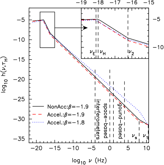
Figure 1: The spectrum $h(k,\tau_{H})$ as a function of the frequency $\nu$ in the present Universe in both accelerating and decelerating expansion.

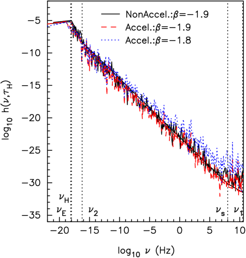
Figure 2: The spectrum $h(k,\tau_{H})$ from the numerical calculation.

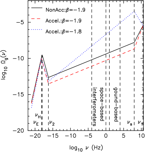
Figure 3: The energy spectrum $\Omega_{g}(\nu)$ in the present Universe in both accelerating and decelerating expansion.

With these results we plot the spectrum $h(k,\tau_{H})$ vs the frequency $\nu$ for two values of parameter $\beta=-1.9,\,-1.8$ in Figure 1. Besides, for convenience of comparison, the spectrum for the decelerating model is also plotted for $\beta=-1.9$. It is clearly seen that, for the same parameter $\beta=-1.9$ in the whole range $\nu\geq\nu_{H}$, the accelerating model has an amplitude lower by a factor of $\sim 2.2$ than that of the decelerating model. This is due to the extra factor $\frac{1}{(1+z_{E})^{3}}=\frac{\Omega_{m}}{\Omega_{\Lambda}}$, as has been demonstrated in the previous expressions (34), (35), and (36). Interestingly, the larger value $\beta=-1.8$ gives a flatter spectrum $h(\nu,\tau_{H})$ with an overall higher amplitude in the range $\nu\geq\nu_{2}$. In particular, in the higher frequency range $(10^{-4}\sim\,0)$ Hz covered by LISA, the amplitude is $h\simeq 10^{-19}\sim 10^{-22}$ for the $\beta=-1.8$ case, about $10$ to $10^{2}$ higher than the $\beta=-1.9$ case. In the even higher frequency range $(10\sim\,10^{4})$ Hz covered by LIGO, the amplitude is $h\simeq 10^{-23}\sim 10^{-25}$ for the $\beta=-1.8$ case, also $10$ to $10^{2}$ higher than the $\beta=-1.9$ case. Thus an inflationary model of larger index $n=2\beta+5$ will predict a stronger signal of relic gravitational waves in higher frequencies.

The recent second science run of the LIGO interferometric detectors [23] gives a sensitivity $3\times 10^{-24}$ to $3\times 10^{-23}$ in the frequency range $(10^{2},\,10^{3})$Hz. The best sensitivity is given by the 4km arm L1 detector located at Livingstone, which is about $3\times 10^{-24}$ near a frequency $\sim 300$Hz. Our calculation for the $\beta=-1.9$ case yields an amplitude, $h\simeq 10^{-26}$, much smaller than this sensitivity of the second run. However, the most interesting case is the model of $\beta=-1.8$, in which the amplitude of the gravitational waves is just to fall into the sensitivity of the L1 detector. Since the second run of LIGO has not observed any signal of stochastic gravitational waves in this frequency range, we arrive at a constraint $\beta\leq-1.8$ on the model parameter of the inflationary expansion. Note that this constraint is also consistent with $\beta<-1.78$, as has been imposed,through Eq.(38), from the observed CMB anisotropies of WMAP.

As a double check, we have also numerically solved the differential equation (6) of the gravitational waves, and have found the resulting power spectrum $h(\nu,t)$ from the numerical solution, which is plotted in Figure 2. Since the numerical result that we have plotted carries the oscillating factor $\cos(2\pi\nu(t-t_{\nu}))$, so its curve shows an extra small zigzag, as expected. Moreover, for the range of small frequencies, $\nu<\nu_{H}$, $\cos(2\pi\nu(t-t_{\nu}))\simeq 1$, the oscillating amplitude is very small, confirming an observation made by ref. [8]. Except for this oscillating effect, the numerical result of the spectrum in Figure 2 agree with the analytical one in Figure 1.

We also plotted the spectral energy density $\Omega_{g}(\nu)$ from the analytic solution in Figure 3. It is similar to the known result, except for the obvious distortions caused by the acceleration of the Universe expansion in the low frequency range .

6. Conclusion.

We have presented a calculation of the spectrum of relic gravitational waves in the present Universe in accelerating expansion. The recent WMAP result of $\Delta T/T$ has been used to normalize the amplitude of relic gravitational waves. In comparison with the decelerating models, the spectrum has been modified due to the particular form of the barrier function $a^{\prime}/a$ during the acceleration of current expansion. Specifically, in very low frequency range $(<\nu_{H})$ the spectrum has been changed with the peak of spectrum being now located at $\nu_{E}$, and there appears a new segment of spectrum from $\nu_{E}$ to $\nu_{H}$. These very long wave length features can be only be possibly detected by the CMB anisotropies at low multipoles. In the higher frequency range $(\geq\nu_{H})$ the spectral amplitude acquires an overall factor $\frac{\Omega_{m}}{\Omega_{\Lambda}}$ as compared with the decelerating model. This higher frequency range is pertinent to the detection projects such as LISA and LIGO. In addition, using the $\Delta T/T$ at low multipoles for normalization gives a larger upper limit $\beta<-1.78$. A larger value of $\beta$ yields a flatter spectrum $h(\nu,\tau_{H})$ as a function of $\nu$, producing more power on the higher frequencies. The resulting sensitivity of the second scientific run of the LIGO detectors, has put a restriction on the model parameter $\beta\leq-1.8$.

ACKNOWLEDGMENT: Y. Zhang’s research work has been supported by the Chinese NSF (10173008) and by NKBRSF (G19990754). Y.F. Yuan is supported by the Special Funds for Major State Research Projects.

References

[1] A.A.Starobinsky, JEPT Lett. 30, 682 (1979).
[2] V.A. Rubakov, M.V.Sazhin, and A.V.Veryaskin,
Phys.Lett.115B, 189 (1982).
[3] R.Fabbri and M.D. Pollock, Phys.Lett. 125B, 445 (1983).
[4] L.F.Abbott and M. B. Wise, Nucl.Phys. B224, 541 (1984);
[5] L.F.Abbott and D.D.Harari, Nucl.Phys. B264, 487 (1986).
[6] B.Allen, Phys.Rev.D 37, 2078 (1988).
[7] V.Sahni Phys.Rev.D 42, 453 (1990).
[8] L.Grishchuk, Class.Quant.Grav. 14 1445 (1997);
Lecture Notes Physics 562, 164 (2001), in “Gyros, Clocks,
Interferometers…:
Testing Relativistic Gravity in Space”, Lammerzahl et al (Eds).
[9] A. Riszuelo and J-P Uzan, Phys.Rev.D 62, 083506, (2000).
[10] H. Tashiro, K. Chiba, and M. Sasaki, Class.Quant.Grav. 21 1761 (2004).
[21] L.Parker, (1979) ”The production of elementary particles by strong
gravitational fields” in “Asymptotic Structure of Space-Time”,
eds. S.Deser and M.Levy (New York: Plenum).