Abundance anomalies in hot horizontal branch stars of the galactic globular cluster NGC 1904

We present abundance measurements, based on high-resolution optical spectroscopic data obtained with the Ultraviolet and Visual Echelle Spectrograph mounted on Kueyen (Very Large Telescope UT2), for ten stars in the extended blue horizontal branch of the Galactic globular cluster NGC 1904 (M79). In agreement with previous findings for other clusters, we obtain normal abundances for stars cooler than $T_{\rm eff}\sim 11\,000$ K, and largely anomalous abundances for hotter stars: large He depletions, and overabundances of Fe, Ti, Cr, P and Mn. The abundances of Mg, Si and Ca are roughly normal, in the hot stars as well as in the cooler ones. This abundance pattern can be attributed to the onset of diffusion and to radiation pressure in the stable atmospheres of hot horizontal branch stars.

1 Introduction

Sandage & Wildey (1967) and van den Bergh (1967) first noticed that the distribution of stars along the horizontal branch (HB) of globular clusters (GCs) cannot be described as a simple uniparametric function of metal abundance. In spite of intensive efforts since then, the additional (second) parameter has not yet been clearly identified; while numerous candidates have been proposed, none of them is sufficient to justify the whole pattern of observations. The issue is likely complicated by several factors. In particular, the distribution of stars along the warmest side of the horizontal branch (i.e. stars bluer than the RR Lyrae instability strip, hence BHB) is very complex, exhibiting a large variety of shapes, from short, stubby horizontal branches (like e.g. in NGC 6397), to very long blue tails (like e.g. in NGC 1904).

The distribution of stars along the HB of a GC is essentially determined by their masses: the smaller the mass, the bluer its colour. Since within a GC, stars have virtually the same age and chemical composition and hence possibly the same mass at the turn-off (see however D’Antona et al. 2002), the colour of stars along the HB should be determined by the amount of mass lost by each star before reaching the HB (the larger the mass lost, the bluer the colour on the HB). While it seems quite reasonable to assume that mass loss occurs more easily in extended and luminous red giants, the mechanisms driving mass loss are far from being well understood, in particular in the case of metal-poor, GC stars. Any possible observation relevant to this topic might help to constrain these mechanisms.

Core rotation (Mengel & Gross 1976; Sweigart & Catelan 1998) is a reasonable candidate for enhanced mass loss along the red giant branch (RGB). In fact, core rotation reduces pressure in the helium cores, delaying the helium flash that terminates evolution along the RGB. Stars with rotating cores may then evolve to brighter luminosities, and have the possibility to lose more mass. We would then expect that descendants of RGB stars with fast core rotation would inhabit the bluest part of the HB. Some support for this hypothesis was given in the ’80s by observation of rotating BHB stars in M13 (a cluster with a bluer than expected HB), but not in M3, by Peterson et al. (1983) and Peterson (1983, 1985a, 1985b). In recent years, with the advent of 8-10 m class telescopes, this issue has been more extensively revisited by Behr et al. (1999, 2000a, 2000b; revised in Behr 2003a, 2003b) and more recently by our group (Recio-Blanco et al. 2002). These additional observations revealed a much more complicated pattern than expected. Fast rotating stars are present also among field HB stars (i.e., this is not an effect limited to globular cluster stars, like the O-Na anticorrelation, see e.g. Kraft 1994), and are present in most clusters (even M3, according to Behr 2003a). They are however found only among the stars cooler than $\sim 11\,500$ K. This temperature value plays an important role in the HB picture: stars warmer than this (and cooler than about 20 000 K) have anomalously bright $u$ magnitudes in Strömgren photometry (Grundahl et al. 1998, 1999); also, gravities derived for these stars from the wings of Balmer and helium lines are systematically lower than predicted by evolutionary models (Moehler et al. 1995, 2003). As shown by several authors (Grundahl et al. 1999; Moehler et al. 1999; Hui-Bon-Hoa et al. 2000), this can be attributed to the onset of strong effects of levitation due to microscopic diffusion and radiation pressure that can be seen in stars lacking significant sub-atmospheric convection zones (Sweigart 2002). When microscopic diffusion and radiation pressure are not overwhelmed by convection, the atmospheres of warm stars are expected to be strongly depleted in He (Greenstein et al. 1967; Michaud et al. 1983), and to exhibit large overabundances of elements like Fe, Ti and P (Turcotte et al. 1998; Richer et al. 2000). All these features are indeed observed (Glaspey et al. 1989; Moehler et al. 1999; Behr 2003a).

It should be noted that most of these results - in particular those related to the chemical composition - have been obtained only for a few GCs, mainly by a single group. It would be useful to extend such observations to more clusters, performing an independent analysis. In this paper we present a new analysis of the chemical composition of 10 BHB stars in the southern cluster NGC 1904 (M79). NGC 1904 is a cluster of intermediate metal abundance ([Fe/H]=-1.59 according to Kraft & Ivans 2003, using Kurucz 1994 models), with an extended very blue HB: these properties are similar to those of M13, one of the clusters studied by Behr (2003b). The observational material obtained by us for NGC 1904 was originally intended only for measurements of the rotational velocities: hence the spectra have a low signal-to-noise ratio ($S/N$), although high resolution. However, we will show that abundances good enough for the purposes of the present discussion could be obtained even from this material.

2 Observations and reduction

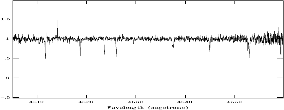
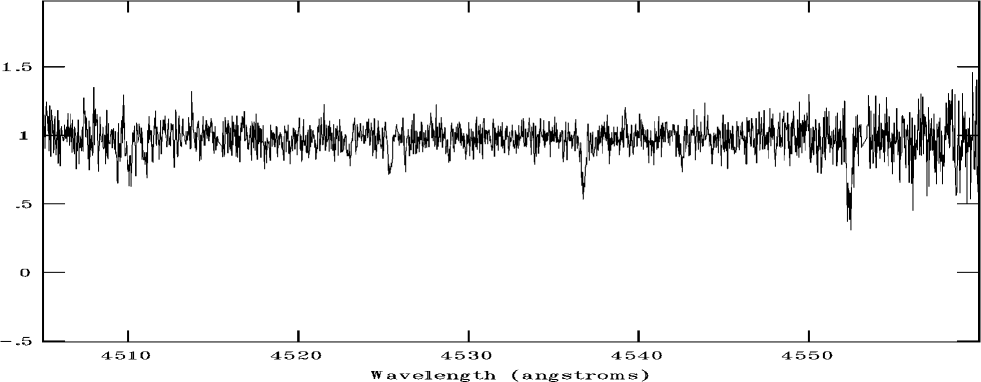
Figure 1: Spectral sections of the stars 392 (top panel), and 209 (bottom panel)

A total of 21 stars were observed in NGC 1904; however, spectra for only 10 of these stars were deemed of good enough quality for abundance analysis, the criteria being the $S/N$ of the spectra and the rotational velocity of the stars (only slow rotators were considered). We selected our targets from the F439W and F555W HST-WFPC2 photometry by Piotto et al. (2002). In addition, we have also identified the NGC 1904 targets in the Strömgren u, y photometry by Grundahl et al. (1999) and the Johnson U, V photometry by Momany et al. (2004). In general, targets lie in the low-density outskirts of the GC, to avoid contamination from other stars. The spectra were obtained during 2 observing runs: July 30–August 2 2000 and January 19–23 2001.

The observations were carried out with the UVES echelle spectrograph, mounted on the Unit 2 (Kueyen) of the VLT, and the 2K x 4K, 15 $\mu$m pixel size blue CCD, with a readout noise of 3.90 e^- and a conversion factor of 2.04 e^-/ADU. The UVES blue arm, with a spectral coverage in the 3730-5000 $\stackrel{{\scriptstyle\circ}}{{\rm A}}$ range, was used. Combined with a slit width of 1.0 arcsec, we achieved a resolution of R$\sim$ 40 000 ($\delta\lambda\sim 0.1\stackrel{{\scriptstyle\circ}}{{\rm A}}$, $\delta v\sim$ 7.5 km/s, see the UVES user manual by Kaufer et al. 2003).

The exposure times ranged from 800 s (for V $\sim$ 16) to 4000 s (for V $\sim$ 17.5). We generally limited individual exposure times to 1500 or 2000 seconds, to minimize cosmic ray accumulation, and then coadded individual frames obtained for each star. The typical signal to noise ratios of the coadded spectra are about 20 to 30 per resolution element, but in a few cases they are as good as $S/N\sim$40-60. See Fig. 1 for a visual example of the quality of the target spectra.

The spectra were extracted using standard IRAF procedures. For the wavelength calibration we fitted 3^rd order polynomials to the dispersion relations of the ThAr calibration spectra, which resulted in residuals of $\leq$ 3$\cdot$10^-4 $\stackrel{{\scriptstyle\circ}}{{\rm A}}$. Finally, each spectrum was normalized using a 5th-degree polynomial fitting.

3 Abundance measurements

We have performed an abundance analysis of 10 stars in M79. The abundance measurements were performed using the program WIDTH3, developed by R. G. Gratton and adapted by D. Fabbian to temperatures up to $T_{\rm eff}\simeq$ 20 000 K (D. Fabbian graduate thesis). The procedure establishes the abundances of chemical species by reproducing the observed equivalent widths. Once a starting set of values for the effective temperature, surface gravity and model metal abundance is derived, an appropriate model for each star is obtained from the grid of model atmospheres by Kurucz (1994) by interpolating linearly in temperature and logarithmically to get the Rosseland opacity, electronic and gaseous pressure, and density. Continuum opacity was obtained taking into account all important continuum opacity sources for stars as hot as $T_{\rm eff}=20\,000$ K. Collisional damping constants were computed with the Uns$\ddot{\rm o}$ld formula. The equation of transfer was then integrated through the atmosphere at different wavelengths along the line profile and theoretical equivalent widths of the lines computed and compared with the observed ones.

3.1 Oscillator strengths, line selection and solar abundances

Only lines free of blends were considered in the analysis. The line list was extracted from the solar spectrum tables by Moore et al. (1966), and the atomic line lists by Hambly et al. (1997) and Kurucz & Bell (1995), more appropriate for warmer stars.

For the determination of the oscillator strengths (gfs), laboratory values were considered whenever possible. For Fe i lines they were taken from papers of the Oxford group (Simmons & Blackwell 1982) and Bard & Kock (1994). The gfs for the Fe ii lines were taken from Heise & Kock (1990) and Biemont et al. (1991), while gfs for the Mg i lines came from Gratton (2003). For the rest of the lines, the gfs were those provided by Kurucz (1994) and the NIST atomic spectra database.

The solar abundances were taken from Grevesse & Sauval (1998).

3.2 Equivalent Widths

Equivalent Widths ($EW$s) were measured on the unidimensional, extracted spectral orders using an automatic routine within the ISA package, prepared by R. Gratton (see Bragaglia et al. 2001). The routine works as follows. First, a local continuum level is determined for each line by an iterative clipping average of the 200 spectral points centered on the line to be measured. Second, the equivalent width for each line from an extensive list is tentatively measured using a Gaussian fitting routine. Measures are rejected according to several criteria (e.g., if the central wavelength does not agree with that expected from a preliminary measure of the geocentric radial velocity or if the lines are too broad or too narrow). Third, the measured lines are used to draw a relationship between equivalent width and FWHM. Fourth, this relation is used to measure equivalent widths again, using a second Gaussian fitting routine that has only one free parameter (the equivalent width), since the central wavelength is fixed by the measured geocentric radial velocity and the FWHM is fixed by the relationship between equivalent width and FWHM. Again measures are rejected if residuals are too large, asymmetric, etc.

But for a few exceptions (Mg ii and Ca ii lines having $EW>$100 mÅ ), only lines with 10$<EW<$100 mÅ were finally considered. Lines with $EW<$30 mÅ were only used for the star 392, the one with the best spectrum (see section 4.2 and Figure 1). The number of measured lines depends on the $S/N$ and on the star’s metallicity. Generally, around 15 Fe i lines and 20 Fe ii were measured. Measured $EW$s for individual stars are listed in Table 1, only available in electronic form.

Table 1: The measured equivalent widths and corresponding uncertainties used in our abundance analysis. The table is available only in electronic form at the CDS. Column 1 lists the chemical elements of interest with their ionization stage; Column 2 gives the corresponding wavelengths (in Å); excitation potentials (in eV) and $\log$ gfs are given in Column 3 and 4 respectively; the measured equivalent widths and corresponding uncertainties (in mÅ) for the 10 stars are listed in the next columns, with a few values being upper limits

Table 2: Abundance errors for the star 392, due to uncertainties $\sigma(\Delta EW)$ in equivalent width, $\sigma(\Delta T)$ in effective temperature, $\sigma(\Delta g)$ in $\log g$, $\sigma(\Delta\xi)$ in $\xi$ and $\sigma(\Delta z)$in [A/H]

Element	$\sigma(\Delta EW)$	$\sigma(\Delta T)$	$\sigma(\Delta g)$	$\sigma(\Delta\xi)$	$\sigma(\Delta z)$
	$\pm 10.4$	$\pm 200$	$\pm 0.1$	$\pm 1$	$\pm 0.1$
	(mÅ)	(K)	dex	km/s	dex
He i	0.3	0.11	0.06	0.02	0.09
Mg ii	0.2	0.02	0.01	0.08	0.00
Si ii	0.2	0.02	0.03	0.03	0.01
P ii	0.2	0.02	0.03	0.05	0.01
Ca ii	0.4	0.05	0.04	0.22	0.01
Ti ii	0.2	0.09	0.00	0.05	0.02
Cr ii	0.2	0.04	0.02	0.03	0.02
Mn ii	0.2	0.03	0.02	0.02	0.01
Fe i	0.2	0.10	0.03	0.05	0.04
Fe ii	0.2	0.02	0.03	0.09	0.01

Due to the quality of the spectra, the $EW$ uncertanties were the most important source of errors in the abundance determinations. This error was evaluated by comparing the equivalent width measurements of the stars 209 and 281. These stars have almost equal atmospheric parameters, with differences just slightly larger than the internal errors. In addition, they do not present signs of diffusive effects in their atmospheres. An analysis of 22 lines measured in both spectra indicates that the mean difference between the two equivalent width measurements is $-1.1$ mÅ (in the sense 281-209), with a standard deviation of 14.7 mÅ. Therefore, assuming that equivalent width errors for both stars are the same, the error for each measurement is 14.7/$\sqrt{2}$=10.4 mÅ. If we compare this result with the value calculated through the Cayrel (1988) formula:

$$\Delta(EW)=1.6\sqrt{(wdx)}/(S/N)$$

with $w$  being the full width at half maximun (FWHM) typical of the lines, in this case $\sim$0.12 Å, and $dx$ being the pixel size, about 0.03 Å, we get $\Delta(EW)\simeq 10$ mÅ (assuming a $S/N\simeq$10 per pixel), which is more or less what we obtained comparing the measurements for the stars 209 and 281. This result implies that identification of the correct continuum level (that is neglected in the Cayrel formula) is not an issue here, as expected since the spectra of BHB stars have very few absorption lines.

Consequently, we calculated the abundance errors, derived from an equivalent width uncertanty of 10.4 mÅ. The resulting errors for the star 392, $\sigma(\Delta EW)$, are shown in Column 2 of Table 2.

3.3 Atmospheric parameters

Figure 2: Colour magnitude diagram for the target stars. Filled symbols are stars for which abundance analysis was done; open symbols are those stars for which only rotational velocities were obtained. Left panel: $U-(U-V)$ colour magnitude diagram from Johnson photometry by Momany et al. (2004). Right panel: $u$,$(u-y)$ diagram from Strömgren photometry by Grundahl et al. (1999). ZAHB models by Cassisi et al. (1999) are plotted as continuous lines. The location of the luminosity jump is marked with an arrow in both CMDs

Table 3: Photometry for all the target stars in NGC 1904. The temperature values derived from the $u$,$(u-y)$ Grundahl et al. (1999) CMD, $T_{\rm effg}$, the corresponding corrected effective temperature values $T_{\rm effgc}$ and the temperature derived from the Momany et al. (2004) CMD, $T_{\rm effm}$

ID	y	b	v	u	V	B	U	$T_{\rm effg}$	$T_{\rm effgc}$	$T_{\rm effm}$
								(K)	(K)	(K)
243	16.23	16.29	16.47	17.96	16.29	16.31	16.44	7700	8684	8500
209	16.06	16.14	16.34	17.85	16.11	16.16	16.29	7500	8537	8400
294	16.24	16.31	16.49	18.00	16.30	16.32	16.46	7600	8611	8600
295	16.37	16.41	16.56	18.02				8000
289	16.32	16.37	16.52	17.96	16.37	16.36	16.45	8100	8976	9000
275	16.25	16.31	16.48	17.97	16.32	16.32	16.44	7700	8684	8800
297	16.46	16.47	16.57	17.85	16.51	16.43	16.39	9300	9853	10200
327	16.43	16.46	16.61	18.00	16.48	16.45	16.50	8400	9195	9400
292	16.25	16.32	16.50	18.00	16.29	16.37	16.49			8400
281	16.35	16.38	16.53	17.96	16.36	16.41	16.49	8200	9049	8800
298	16.35	16.38	16.53	17.97	16.37	16.40	16.48	8200	9049	8900
489	17.34	17.31	17.35	17.86	17.42	17.24	16.72	14500	13654	13000
354	16.64	16.67	16.79	17.93	16.73	16.67	16.58	9800	10219	10600
469	17.11	17.10	17.16	18.00	17.17	17.03	16.71	12300	12046	12200
434	16.92	16.92	16.99	17.78	16.99	16.86	16.61	12300	12046	11600
389	16.71	16.70	16.77	17.78	16.77	16.65	16.43	11000	11096	11200
363	16.90	16.92	17.01	17.88	17.45	17.32	17.07	11800	11681
366	16.61	16.62	16.74	17.99	16.67	16.61	16.56	9400	9926	10200
555	17.55	17.51	17.56	18.18	17.60	17.44	16.99	13700	13070	13800
392	16.74	16.74	16.81	17.68	16.82	16.67	16.37	12100	11900	11500
535	17.47	17.47	17.54	18.08	18.07	18.14	17.50	13700	13070

Model atmospheres appropriate for each star were extracted from the grid of Kurucz (1994). Figure 2 shows the projections of the analyzed HB stars into the corresponding zero age horizontal branches (ZAHBs) for the two adopted photometries. The position of the Grundahl et al. (1999) luminosity jump is marked with a vertical arrow. This feature clearly affects the fit of the models to the observed HBs, especially in the $u$,$(u-y)$ CMD. $T_{\rm eff}$ values were determined from the position of the stars in the $u$,$(u-y)$ CMD by Grundahl et al. (1999), and the position in a Johnson $U$,($U-V$) CMD by Momany et al. (2004), using the ZAHB models by Cassisi et al. (1999), see Fig. 2. Those models were transformed from the theoretical plane to the observational one using the colour-effective temperature relation provided by Castelli et al. (1997a,b). Hereafter, we adopt a reddening value of $E(B-V)=0.01$, from the Harris (1996) compilation. The value that could be obtained using the maps of Schlegel et al. (1998) based on COBE-DIRBE data is $E(B-V)=0.031$. If we had rather adopted this last value of the interstellar reddening, the temperatures would have been $\sim 200$ K warmer; this is less than the internal errors.

Table 3 presents the photometric parameters for all 21 stars in NGC 1904 for which we obtained spectra, with the corresponding temperature values derived from the Grundahl et al. (1999) $u$,$(u-y)$ CMD and the Momany et al. (2004) CMD, respectively labelled $T_{\rm effg}$ and $T_{\rm effm}$. Only 10 of these stars, selected among the slow rotating ones, were used in the abundance analysis.

Table 4: Atmospheric parameters for stars in NGC 1904

star	$T_{\rm eff}$	$\log g$	$[$A/H$]$	$\xi$
	(K)			(km/s)
209	8469$\pm$200	3.2$\pm$0.2	-1.4	2.4$\pm$1.0
281	8925$\pm$200	3.3$\pm$0.2	-1.4	2.3$\pm$1.0
354	10409$\pm$200	3.7$\pm$0.1	-1.4	2.0$\pm$1.0
389	11148$\pm$200	3.8$\pm$0.1	0.0	0.0$\pm$1.0
363	11681$\pm$300	3.9$\pm$0.1	0.0	0.0$\pm$1.0
392	11700$\pm$200	3.9$\pm$0.1	0.0	0.0$\pm$1.0
434	11823$\pm$200	3.9$\pm$0.1	0.0	0.0$\pm$1.0
469	12123$\pm$200	4.0$\pm$0.1	0.0	0.0$\pm$1.0
535	13070$\pm$300	4.1$\pm$0.1	0.0	0.0$\pm$1.0
489	13327$\pm$200	4.2$\pm$0.1	0.0	0.0$\pm$1.0

To derive the final effective temperature of the programme stars, we calculate the mean of Momany’s temperatures and of Grundahl’s temperatures after transposing these last to Momany’s scale. The final error is the scatter of the temperatures involved in the mean. We decided to convert the $T_{\rm effg}$ values to Momany’s scale mainly because the $T_{\rm effg}$ scale presented a number of problems. For instance, the $T_{\rm effg}$ temperature for the coolest stars would place them inside the RR Lyrae instability strip, and the corresponding metallicity for such a cool temperature would be lower than what is reported for the RGB stars in the cluster. On the other hand, apart from this shift to cooler temperatures, probably due to the ZAHB model fit, all of our targets were well identified in the Grundahl et al. photometry, while 3 of the stars in Momany’s photometry were blended. For this reason, and to be sure of an internal consistency in all the temperature measurements, we decided to transform the $T_{\rm effg}$ values into Momany’s scale, and then calculate the mean, for each star, of the new $T_{\rm effg}$ obtained and the $T_{\rm effm}$ value.

The relation between $T_{\rm effg}$ and $T_{\rm effm}$ was found by averaging the best fit relations obtained assuming the two quantities as independent variables, because internal errors in $T_{\rm effm}$ and $T_{\rm effg}$ were expected to be comparable. The final relation is:

$$T_{\rm effgc}=(0.731\pm 0.039)T_{\rm effg}+(3055\pm 357)\leavevmode\nobreak\ \leavevmode\nobreak\ \leavevmode\nobreak\ {\rm K}$$ (1)

where $T_{\rm effgc}$ is the corrected effective temperature derived from the Strömgren u, y photometry by Grundahl et al. (1999). Internal errors in these temperatures may be obtained by comparing the differences between the temperatures obtained from the two photometries. The r.m.s. average of these differences (taking into account the two degrees of freedom lost because we corrected the temperatures obtained from Grundahl’s photometry to those obtained from Momany’s photometry) is 355 K; assuming that individual errors are similar in the two determinations, the expected internal errors are $\pm 177$ K for those stars with both determinations, and $\pm 251$ K for stars having only Grundahl’s photometry. Hereafter, we will round these values to $\pm 200$ and $\pm 300$ K respectively, see Table 4.

Figure 3: Runs of $T_{\rm eff}$ against the dereddened Johnson $B-V$ color (left panel) and absolute $M_{V}$ magnitude (right panel) for our program stars in NGC 1904 (filled symbols), and for the stars in M13 analyzed by Behr (2003a) (open symbols)

In order to compare the effective temperatures adopted throughout this paper with those adopted in other abundance analyses of BHB stars, we plotted (see Fig. 3, left panel) the runs of $T_{\rm eff}$ against the dereddened Johnson $B-V$ color and of the absolute $M_{V}$ magnitude for both our program stars in NGC 1904 and the stars in M13 analyzed by Behr (2003a). The reddenings adopted here are those from the Harris (1996) compilation. There is a reasonable agreement between the two sets for the coolest stars, while our temperatures for the hottest ones are lower than those obtained by Behr for stars of similar $B-V$ colours. This difference is likely due to some differences in the colour calibration; in fact, the agreement between the two sets is excellent if absolute $M_{V}$ magnitudes are considered (see Fig. 3, right panel).

Gravities are not well costrained by our spectra: in fact equilibrium of ionization is subject to possible departures from LTE, and the Balmer lines are too broad for reliable determinations of their profile from our Echelle spectra. We have then derived a mean relation between $\log T_{\rm eff}$ and gravity ($\log g$) from Behr et al. (1999) measurements of blue HB stars in M13 that were expected to be very similar to those in NGC 1904 on the basis of the colour-magnitude diagram:

$$\log g=4.83\cdot\log T_{\rm eff}-15.74$$ (2)

Figure 4: Comparison between the gravities adopted in this paper ($\log g_{\rm fit}$) and those obtained from the location of the stars in the colour-magnitude diagram, using theoretical models by Cassisi et al. (1999: $\log g_{\rm teo}$)

Figure 4 compares the gravities obtained using this method (and used by us in the abundance determinations), with those that could be derived from photometric angular diameter. In the latter case, a distance modulus of (m-M)${}_{V}=15.59$ (Harris, 1996, in the revised version of 2003) has been adopted for the cluster, and a reasonable mass for the stars was estimated from HB models by Cassisi et al. (1999) for the Johnson photometry, again using the location of the stars in the colour-magnitude diagram. The agreement between these two values is very good, supporting the gravity estimates adopted throughout this paper. Errors in the gravities due to errors in the temperatures are of about 0.05 dex.

Microturbulent velocities $\xi$ might be derived by eliminating trends of the derived abundances with expected line strength for some given species. However, given the quality of our spectra, generally too few lines could be measured, and with too large scatter, to significantly constrain microturbulent velocity. For the cooler stars, we relied on Behr’s analysis of M13 stars. From his analysis, we derived the following relation between $\log T_{\rm eff}$ and the microturbulence velocity:

$$\xi=-4.7\cdot\log T_{\rm eff}+20.9\leavevmode\nobreak\ \leavevmode\nobreak\ \leavevmode\nobreak\ {\rm km/s}$$ (3)

Uncertainties in these values for the microturbulent velocities can be obtained from the scatter of individual values around this mean relation: this is $\sim 1$ km/s. For the warmer stars, we adopted no microturbulent velocity, as given by the analysis of star 392, which has the best spectrum (see Section 4.2).

Metallicities were obtained varying the metal abundance [A/H] of the model until it was close to the derived [Fe/H] value. The adopted atmospheric parameters are listed in Table 4. The errors.

Once $T_{\rm eff}$, $\log g$, $\xi$ and atmospheric [Fe/H] were determined, we calculated the mean abundance and dispersion for each element. Since the abundances for each element depend upon the adopted parameters, we recalculated the abundances varying each of these parameters in turn, to test how much the abundances change. The resulting errors for the star 392 are shown in Table 2, Columns 3 to 6.

4 Results

Table 5: Abundances for stars in NGC 1904. The superscripts next to the abundance determinations indicate the number of lines used in each case

star	log He	log Mg	log Si	log P	log Ca	log Ti	log Cr	log Mn	log Fe
209	…	6.4$\pm$0.32	6.2$\pm$0.21	…	5.7$\pm$0.31	3.7$\pm$0.213	4.4$\pm$0.21	$<4.7$ 1	6.03$\pm$0.209
281	…	6.7$\pm$0.32	6.5$\pm$0.23	…	…	3.9$\pm$0.212	4.8$\pm$0.31	…	6.14$\pm$0.207
354	11.3$\pm$0.31	6.2$\pm$0.32	6.4$\pm$0.22	…	5.4$\pm$0.31	4.3$\pm$0.25	…	…	6.34$\pm$0.206
389	…	6.5$\pm$0.32	7.3$\pm$0.31	7.4$\pm$0.31	5.6$\pm$0.31	4.9$\pm$0.28	…	…	7.90$\pm$0.2014
363	$<9.4$1	6.2$\pm$0.32	…	…	6.3$\pm$0.31	5.3$\pm$0.25	…	…	8.00$\pm$0.2013
392	10.9$\pm$0.31	6.3$\pm$0.32	5.2$\pm$0.22	6.8$\pm$0.36	5.7$\pm$0.31	4.8$\pm$0.212	4.9$\pm$0.33	6.2$\pm$0.21	7.93$\pm$0.2048
434	$<9.3$1	6.5$\pm$0.32	6.1$\pm$0.32	…	6.0$\pm$0.31	5.1$\pm$0.26	6.5$\pm$0.51	…	7.90$\pm$0.2024
469	9.8$\pm$0.31	6.7$\pm$0.32	6.6$\pm$0.21	…	6.0$\pm$0.22	5.4$\pm$0.27	5.8$\pm$0.52	6.5$\pm$0.31	8.11$\pm$0.2028
535	9.8$\pm$0.31	6.2$\pm$0.32	7.2$\pm$0.24	…	5.8$\pm$0.31	4.6$\pm$0.21	…	…	7.90$\pm$0.203
489	9.8$\pm$0.31	6.6$\pm$0.32	7.1$\pm$0.23	6.7$\pm$0.31	6.2$\pm$0.31	5.6$\pm$0.22	7.4$\pm$0.31	…	7.87$\pm$0.2021

Table 6: Abundance relative to solar for stars in NGC 1904

star	[He/H]	[Mg/H]	[Si/H]	[P/H]	[Ca/H]	[Ti/H]	[Cr/H]	[Mn/H]	[Fe/H]
209	…	-1.1$\pm$0.2	-1.3$\pm$0.2	…	-0.6$\pm$0.3	-1.3$\pm$0.2	-1.3$\pm$0.2	$<-0.7$	-1.48$\pm$0.20
281	…	-0.8$\pm$0.2	-1.0$\pm$0.2	…	…	-1.1$\pm$0.2	-0.9$\pm$0.3	…	-1.37$\pm$0.20
354	+0.3$\pm$0.3	-1.3$\pm$0.2	-1.1$\pm$0.2	…	-0.9$\pm$0.3	-0.7$\pm$0.2	…	…	-1.17$\pm$0.20
389	…	-1.0$\pm$0.2	-0.2$\pm$0.3	+1.9$\pm$0.3	-0.7$\pm$0.3	-0.1$\pm$0.2	…	…	+0.39$\pm$0.20
363	$<-1.6$	-1.3$\pm$0.2	…	…	0.0$\pm$0.3	+0.3$\pm$0.2	…	…	+0.49$\pm$0.20
392	-0.1$\pm$0.3	-1.2$\pm$0.2	-2.3$\pm$0.2	+1.3$\pm$0.3	-0.6$\pm$0.3	-0.2$\pm$0.2	-0.8$\pm$0.3	+0.8$\pm$0.2	+0.42$\pm$0.20
434	$<-1.7$	-1.0$\pm$0.2	-1.4$\pm$0.2	…	-0.3$\pm$0.3	+0.1$\pm$0.2	+0.8$\pm$0.5	…	+0.39$\pm$0.20
469	-1.2$\pm$0.3	-0.8$\pm$0.2	-0.9$\pm$0.3	…	-0.3$\pm$0.2	+0.4$\pm$0.2	+0.1$\pm$0.5	+1.1$\pm$0.3	+0.60$\pm$0.20
535	-1.2$\pm$0.3	-1.3$\pm$0.2	-0.3$\pm$0.2	…	-0.5$\pm$0.3	-0.4$\pm$0.2	…	…	+0.39$\pm$0.20
489	-1.2$\pm$0.3	-0.9$\pm$0.2	-0.4$\pm$0.2	+1.2$\pm$0.3	-0.1$\pm$0.3	+0.6$\pm$0.2	+1.7$\pm$0.3	…	+0.36$\pm$0.20

4.1 Abundance anomalies

In this section we present the results of the abundance analysis. Tables 5 and 6 contain the abundance values derived for each of our target stars, both on an absolute scale, and relative to the solar abundances of Grevesse & Sauval (1998). The scatter of the measurements for the corresponding lines gives the quantity $\sigma_{N}$, which is added quadratically to the error contributions in $T_{\rm eff}$, $g$, $\xi$ and [A/H] described in the previous chapter, to get the final error for each element in each target star.

4.2 Star 392

Figure 5: Curve of growth for Fe ii lines in the spectrum of star 392

Figure 6: Upper panel: run of the extracted abundances for individual Fe ii lines from the spectrum of star 392 with excitation potential (in EV). Lower panel: the same, but against expected line strength

We will first consider the analysis of star 392, whose spectrum has the highest $S/N$ ($\sim 60$ per resolution element at a wavelength of 4240 Å). For this star we were able to measure over 100 lines.

Figure 5 shows the curve of growth of Fe ii. Clearly, many unsaturated lines were accurately measured. As shown in Figure 6, no trend was detected in the number of Fe atoms, log n(Fe), with the excitation potential, as expected for the excitation equilibrium. This test is very critical, given the large spread of excitation potentials (nearly 10 eV): even a modest error of 500 K in the effective temperature would result in a very significant trend in this plot.

The large number of measured lines for Fe ii allowed an accurate estimate of the microturbulent velocity: best results were obtained setting it to zero (i.e., leaving only thermal broadening as an unsaturating factor). This result is not surprising in view of the fact that this star is so hot that the atmosphere should be in radiative equilibrium.

With our value of the effective temperature and surface gravity, we got an excellent equilibrium of ionization for Fe: the mean abundance given by neutral lines is log n(Fe)=$7.86\pm 0.03$ (31 lines, r.m.s. of results for individual lines of 0.18 dex), while that obtained from singly ionized lines is log n(Fe)=$7.93\pm 0.03$ (48 lines, r.m.s. of results for individual line of 0.20 dex). The offset between the abundances is only marginally larger than the sum of the internal errors; again, a small change of the effective temperatures and gravities (within the internal errors of both these quantities) would bring the two abundances in agreement with each other.

This very good agreement supports our LTE analysis. Actually, such a good agreement was not foreseen, since we expected some overionization of Fe, leading to lower abundances from neutral lines in an LTE analysis. This result should be compared with appropriate predictions from statistical equilibrium calculations for these stars; however, this is beyond the scopes of the present analysis.

4.3 Other stars

The abundance values for the various elements for which we have data are plotted in Figures 8, 9, 10, 11. In the upper panels, the abundances for individual stars in NGC 1904 are plotted as a function of $T_{\rm eff}$ as log offsets from the solar abundances. The abundance values from Behr (2003a) for M13 are plotted for comparison in the lower panels. The horizontal lines represent the expected value of [metal/H] from solar for NGC 1904 and M13 in the Carretta & Gratton (1997) scale: at -1.37 and -1.39, respectively. For helium, the horizontal line represents the solar ratio. We used the abundances derived from lines of the dominant ionization stage of each element, to minimize the possibility of non-LTE effects.

4.3.1 Iron, titanium and chromium

Table 7: Statistics of Fe Abundances

star	Fe i			Fe ii
	n	$<>$	$\sigma$	n	$<>$	$\sigma$
209	29	6.06	0.19	9	6.03	0.25
281	19	6.47	0.27	7	6.14	0.26
354	2	6.90	0.18	6	6.34	0.32
389	11	7.66	0.27	14	7.90	0.31
363	8	8.24	0.47	13	8.00	0.38
392	31	7.86	0.18	48	7.93	0.20
434	9	7.80	0.44	24	7.90	0.48
469	9	7.87	0.26	28	8.11	0.34
535				3	7.90	0.06
489				21	7.87	0.46

Figure 7: Differences between abundances for Fe i and Fe ii lines as a function of temperature

Figure 8: Abundance values for iron, titanium and chromium as a function of $T_{\rm eff}$ as log offsets from the solar abundances. The abundance values from Behr et al. (2003a) for M13 are also plotted for comparison in the lower panels. The horizontal solid lines represent the expected value of [metal/H] from solar for NGC 1904 and M13, in the Carretta & Gratton (1997) scale. The arrows at 11 000 K indicate the approximate position of Grundahl’s photometric jump

Statistics of abundances for Fe are given in Table 7. Abundances are obtained from both neutral and singly ionized lines, in a few cases from a total of more than 30 lines. Figure 7 displays the run of the differences between the average abundances obtained from neutral and singly ionized Fe lines as a function of temperature. Abundances from Fe i lines agree well with those from Fe ii lines. However, given the possibility that small non-LTE effects are present, in the following discussion we considered the abundances provided by singly ionized Fe, which is the dominant species and should then be less affected by model uncertainties.

As can be seen from Figure 8, the iron abundances for the three coolest stars are very close to the cluster metallicity from analysis of red giant branch stars. We obtain [Fe/H]=$-1.48$, $-1.37$, and $-1.17$, yielding an average value of [Fe/H]=$-1.34\pm 0.09$. This value may be compared with those obtained from analysis of red giants: [Fe/H]=-1.37 on the Carretta & Gratton (1997) scale and the slightly lower value of [Fe/H]=-1.59 given by Kraft & Ivans (2003).

On the other hand we find remarkable enhancements of iron and other metal species among the blue HB stars hotter than $\sim$ 11 000 K. The coolest star showing signs of radiative levitation is star 389 at $T_{\rm eff}=11\,148\pm 200$ K, with a supra-solar value of [Fe/H]$=+0.39\pm 0.20$. Stars hotter than $\sim$11 000 K show a very similar iron content: the average value is [Fe/H]=$+0.43\pm 0.05$. The very small scatter (0.08 dex) may be justified by the internal errors in the atmospheric parameters. Both the threshold temperature at which the anomalous abundances appear, as well as the amplitude of the enhancement (about 1.8 dex) are similar to those found by Behr et al. (2003a) for various clusters.

In a similar way, titanium is found a few tenths of a dex above the cluster baseline in the cooler stars ([Ti/H]=-1.3, -1.1, and -0.7). The average value of [Ti/Fe]=+0.31 agrees very well with the overabundance of this element as generally found in cooler metal-poor stars. Titanium abundances then rise by a factor quite similar to that found for Fe in the hotter population.

A similar trend is also obtained for chromium, again in good agreement with the results by Behr (2003a); however, Cr abundances are based on only two Cr ii lines.

4.3.2 Helium

Figure 9: Same as Figure 8, but for Helium

The He abundances appear below the expected solar He/H ratio in the stars with $T_{\rm eff}>11\,000$ K. However, at variance with the case of Fe, we found a large and likely significant star-to-star scatter in the He depletions, see Fig.  9. The case of star 392 is very significant: the relatively high $S/N$ allows clear detection of the He lines. The He abundance we derive from the 4471 Å line is consistent with the solar value. On the other hand, no He line at all was detected in other stars having a similar temperature. Weak lines were detected in the spectra of the warmer stars, suggesting a large He depletion of at least an order of magnitude.

4.3.3 Phosphorus and manganese

Figure 10: Same as Figure 8, but for phosphorus and manganese

Some metals, such as phosphorus and manganese (see Fig. 10), display significantly larger enhancements than iron. We do not observe any P ii line among the cooler stars, but if we assume an appropriately-scaled solar composition for these stars, then the supra-solar value of [P/H] $\simeq$ +1.5 that we find for the hot stars implies an enhancement of $\sim$3 orders of magnitude with respect to the cluster’s adopted metallicity. It is worth noting that several P ii lines were found in the field HB stars Feige 86 and 3 Cen A by Sargent & Searle (1967) and Bidelman (1960), respectively, suggesting that the same mechanism may be at work in both cluster stars and field stars. On the other hand, Behr (2003a) found very similar P enhancements for hot HB stars in M13. Similar very large overabundances are also observed for manganese.

4.3.4 Magnesium, silicon and calcium

Figure 11 displays the run of the abundances of magnesium, silicon and calcium with temperature. The abundance of magnesium was obtained from the strong multiplet of Mg ii at 4481 Å, that is partially resolved in our spectra; Ca abundance was derived from the resonance K-line.

The abundances for magnesium, silicon and calcium, both below and above the critical temperature of 11 000 K, are consistent with very little or no enhancement, but with a large, likely real scatter for Si. This result agrees with that found by Behr (2003a) and with theoretical expectations.

Figure 11: Same as Figure 8, but for magnesium, silicon and calcium

5 Discussion and conclusions

The abundance anomalies in NGC 1904 are likely to be due to the same diffusion processes that were invoked by Behr et al. (1999): radiative levitation of metals and gravitational settling of helium, in the stable non-convective atmospheres of the hotter, higher gravity stars, as hypothesized by Michaud et al. (1983). In addition, the jump in the $u$,$(u-y)$ diagram by Grundahl et al. (1999) for NGC 1904 is reported at $\log T_{\rm eff}=4.06\pm 0.01$, in very good agreement with the onset of the abundance anomalies observed here.

An underabundance of helium on the BHB was observed in several previous instances (Baschek 1975; Heber 1987; Glaspey et al. 1989; among others) and in fact appears to be typical of stars of this type. Michaud et al. (1983), building on the original suggestion by Greenstein et al. (1967), explained these underabundances as a result of the gravitational settling of helium, which can take place if the outer atmosphere of the star is sufficiently stable. Our current results confirm a distinct trend in [He/H] with $T_{\rm eff}$ and $\log g$ along the HB. Helium depletion is accompanied by photospheric enhancement of metals, since the same stable atmosphere that permits gravitational settling also allows the levitation of elements with large radiative cross sections. Elements which have sufficiently large cross-sections to the outgoing radiation field will experience radiative accelerations greater than gravity and will diffuse upwards, enriching the photosphere. The gross behaviour of the diffusion models can be understood by considering the migration of chemical species in a stellar atmosphere (Gonzalez et al. 1995; Michaud et al. 1983 and Seaton 1997). The relative amount of levitation experienced by each element can be estimated by summing the predicted equivalent widths for each line over the visible and near UV spectral range. The magnitudes of these net equivalent widths suggest that helium will experience only a weak levitation force, insufficient to oppose gravity, magnesium will be levitated by an intermediate amount, perhaps balanced by gravity, while iron will be strongly levitated. This is admittedly a crude approach to what we see in NGC 1904, and Behr et al. measurements in various clusters.

The identification of the detected spectral lines was successful in most cases. A few weak lines were not identified, which could be due to the low S/N of the spectra. Since the abundances of metals we derived are very peculiar, it is possible that other metal species (usually not observed in late B-type stars) are also present in the atmospheres of these hot BHB stars, but based on our data we cannot draw any conclusions about this. Very weak lines were used only for the star having the best spectrum. Our results thus do not change if we remove the abundance determinations from those weak lines.

In general, our abundance measurements in NGC 1904 give very similar results to those obtained previously by Behr et al. (1999) in M13, which, on the other hand, has a very similar metallicity to that of NGC 1904. The very small scatter in Fe abundances among the warmer stars is particularly intriguing. While it could be the result of small statistics, it might indicate that the stars warmer than 11 000 K observed in NGC 1904 all rotate at very similar rates. In fact, Michaud (2002, private comunication) estimates that small differences of about 2-3 km/s in rotational velocity could generate sizeable discrepancies in the radiative levitation and gravitational settling processes. Unfortunately, the accuracy of our rotational measurements in NGC 1904, with errors of the order of 4-5 km/s, do not allow us to explore this possibility.

- (1) Bard, A., & Kock, M. 1994, A&A, 282, 1014
- (2) Baschek, B. 1975, in Problems in stellar atmospheres and envelopes, Springer, New York, p.101
- (3) Behr, B. B. 2003a, ApJS, 149, 67
- (4) Behr, B. B. 2003b, ApJS, 149, 101
- (5) Behr, B. B., Cohen, J. G., McCarthy, J. K., & Djorgovski, S. G. 1999, ApJL, 517, L31
- (6) Behr, B. B., Djorgovski, S. G., Cohen, J. G., et al. 2000, ApJ, 528, 849
- (7) Behr, B. B., Cohen, J. G., & McCarthy, J. K. 2000b, ApJL, 531, L37
- (8) Bidelman, W. P. 1960, PASP, 72, 24
- (9) Biemont, E., Baudoux, M., Kurucz, R. L., Ansbacher W. & Pinnington, E. H. 1991, A&A, 249, 539
- (10) Bragaglia, A., Carretta, E., Gratton, R. G., et al. 2001, AJ, 121, 327
- (11) Brown, T. M., Bowers, C. W., Kimble, R. A., & Ferguson, H. C. 2000, ApJL, 529, L89
- (12) Brown, T. M., Sweigart, A. V., Lanz, T., Landsman, W. B., & Hubeny, I. 2001, ApJ, 562, 368
- (13) Carretta, E., & Gratton, R. G. 1997, A&AS, 121, 95
- (14) Cassisi, S., Castellani, V., degl’Innocenti, S., Salaris, M., & Weiss, A. 1999, A&AS, 134, 103
- (15) Castelli, F., Gratton, R. G., Kurucz, R. L. 1997, A&A, 318, 841
- (16) Castelli, F., Gratton, R. G., Kurucz, R. L. 1997, A&A, 324, 432
- (17) Cayrel, R. 1988, in The Impact of Very High S/N Spectroscopy on Stellar Physics, IAU Symp. 132, eds. G. Cayrel de Strobel & M. Spite, Kluwer, Dordrecht, p. 345
- (18) Crocker, D. A., Rood, R. T., O’Connell, R. W. 1988, ApJ, 332, 236
- (19) D’Antona, F., Caloi, V., Montalban, J., Ventura, P., & Gratton, R. 2002, A&A, 395, 69
- (20) Dixon, W. V., Davidsen, A. F., Dorman, B., Ferguson, H. C. 1996, AJ 111, 1936
- (21) Glaspey, J. W., Michaud, G., Moffat, A. F. & Demers, S. 1989, ApJ, 339, 926
- (22) Gonzalez, J.-F., Artru, M.-C., & Michaud, G. 1995, A&A, 302, 788
- (23) Gratton, R. G., Carretta, E., Claudi, R., Lucatello, S., & Barbieri, M. 2003, A&A, 404, 187
- (24) Greenstein, G. S., Truran, J. W. & Cameron, A. G. W. 1967, Nature, 213, 871
- (25) Grevesse, N., & Sauval, A. J. 1998, Space Science Reviews, 85, 161
- (26) Grundahl, F., Vandenberg, D. A., & Andersen, M.I. 1998, ApJ, 500, L179
- (27) Grundahl, F., Catelan, M., Landsman, W. B., Stetson, P. B., & Andersen, M. I. 1999, ApJ, 524, 242
- (28) Hambly, N. C., Rolleston, W. R. J., Keenan, F. P., Dufton, P. L., & Saffer, R. A. 1997, ApJS, 111, 419
- (29) Harris, W. E. 1996, AJ, 112, 1487
- (30) Heber, U. 1987, Mitt. Astron. Ges., 70, 79
- (31) Heise, C., & Kock, M. 1990, A&A, 230, 244
- (32) Hui-Bon-Hoa, A., LeBlanc, F., & Hauschildt, P. H. 2000, ApJ, 535, L43
- (33) Kaufer, A., D’Odorico, S., & Kaper, L. 2003, UV-visual Echelle Spectrograph User Manuali, Doc. No. VLT-MAN-ESO-13200-1825, Issue 1.7, ed. S. Hubrig & C. Ledoux
- (34) Kraft, R. P. 1994, PASP, 106, 553
- (35) Kraft, R. P., & Ivans, I. I. 2003, PASP, 115, 143
- (36) Kurucz, R. 1994, CD-ROM 19, Smithsonian, Cambridge
- (37) Kurucz, R., & Bell, B. 1995, CD-ROM 23, Smithsonian, Cambridge
- (38) Mengel, J. G. & Gross, P. G. 1976, Ap&SS, 41, 407
- (39) Michaud, G., Vauclair, G., & Vauclair, S. 1983, ApJ, 267, 256
- (40) Moehler, S., Heber, U., & DeBoer, K.S. 1995, A&A, 294, 65
- (41) Moehler, S., Heber, U., Rupprecht, G. 1997, A&A, 319, 109
- (42) Moehler, S., Sweigart, A. V., Landsman, W. B., Heber, U., & Catelan, M. 1999, A&A, 346, 1
- (43) Moehler, S., Sweigart, A. V., Landsman, W. B., & Heber, U. 2000, A&A, 360, 120
- (44) Moehler, S., Landsman, W. B., Sweigart, A. V., & Grundahl, F. 2003, A&A, 405, 135
- (45) Momany, Y., Bedin, L. R., Cassisi, S., Piotto, G., Ortolani, S., Recio-Blanco, A., De Angeli, F., & Castelli, F. 2004, A&A, 420, 605
- (46) Moore, C. E., Minnaert, M. G. J., & Houtgast, J. 1966, NBS Monog., Washington
- (47) Peterson, R. C. 1983, ApJ, 275, 737
- (48) Peterson, R. C. 1985a, ApJ, 289, 320
- (49) Peterson, R. C. 1985b, ApJ, 294, 35
- (50) Peterson, R. C., Tarbell, T. D., & Carney, B. W. 1983, ApJ, 265, 972
- (51) Recio-Blanco, A., Piotto, G., Aparicio, A., & Renzini, A. 2002, ApJ, 572, L71
- (52) Richer, J., Michaud, G., & Turcotte, S. 2000, ApJ, 529, 338
- (53) Sandage, A. R., & Wildey, R. 1967, ApJ, 150, 469
- (54) Sargent, W. L. W. & Searle, L. 1967, ApJL, 150, L33
- (55) Schlegel, D. J., Finkbeiner, D. P., & Davis, M. 1998, ApJ, 500, 525
- (56) Seaton, M. J. 1997, MNRAS, 289, 700
- (57) Sills, A., & Pinsonneault, M. H. 2000, ApJ, 540, 489
- (58) Simmons, G. J., & Blackwell, D. E. 1982, A&A, 112, 209
- (59) Sweigart, A. V. 2002, in Highlights of Astronomy, Vol 12, ed. H. Rickman, ASP, S. Francisco, p. 292
- (60) Sweigart, A. V., & Catelan, M. 1998, ApJ, 501, 63
- (61) Turcotte, S., Richer, J., & Michaud, G. 1998, ApJ, 504, 559
- (62) van den Bergh, S. 1967, AJ, 72, 70