The D/H Ratio toward PG 0038+199^1,2

Abstract

We determine the D/H ratio in the interstellar medium toward the DO white dwarf PG 0038$+$199 using spectra from the Far Ultraviolet Spectroscopic Explorer (FUSE), with ground-based support from Keck HIRES. We employ curve of growth, apparent optical depth and profile fitting techniques to measure column densities and limits of many other species (H₂, Na I, C I, C II, C III, N I, N II, O I, Si II, P II, S III, Ar I and Fe II) which allow us to determine related ratios such as D/O, D/N and the H₂ fraction. Our efforts are concentrated on measuring gas-phase D/H, which is key to understanding Galactic chemical evolution and comparing it to predictions from Big Bang nucleosynthesis. We find column densities $\log N(\mbox{{H~{}I}})=20.41\pm 0.08$, $\log N(\mbox{{D~{}I}})=15.75\pm 0.08$ and $\log N(\mbox{H${}_{2}$})=19.33\pm 0.04$, yielding a molecular hydrogen fraction of $0.14\pm 0.02$ ($2\sigma$ errors), with an excitation temperature of $143\pm 5$ K. The high H I column density implies that PG 0038$+$199 lies outside of the Local Bubble; we estimate its distance to be $297^{+164}_{-104}$ pc ($1\sigma$). [D I + HD]/[H I + 2H₂] toward PG 0038$+$199 is $1.91^{+0.52}_{-0.42}\times 10^{-5}$ ($2\sigma$). There is no evidence of component structure on the scale of $\Delta v>8$ km s^-1 based on Na I, but there is marginal evidence for structure on smaller scales. The D/H value is high compared to the majority of recent D/H measurements, but consistent with the values for two other measurements at similar distances. D/O is in agreement with other distant measurements. The scatter in D/H values beyond $\sim 100$ pc remains a challenge for Galactic chemical evolution.

1 Introduction

The ratio of D/H in the interstellar medium (ISM) offers a means to measure the effects of supernovae, stellar winds, infalling halo gas and ISM mixing on the chemical evolution of the Galaxy. The primordial D/H ratio is a firm prediction of the cosmic baryon density from Big Bang nucleosynthesis (Schramm & Turner, 1998; Burles, 2000; Burles et al., 2001). Measuring the D/H ratio in environments as close to primordial as possible in practice means making determinations in low metallicity, high redshift QSO absorbers. Kirkman et al. (2003), building on published work (O’Meara et al., 2001; Pettini & Bowen, 2001; Levshakov et al., 2002) determined primordial $\mbox{{\rm D/H}}=(2.78^{+0.44}_{-0.38})\times 10^{-5}$ ($1\sigma$) which is consistent with WMAP results and Big Bang nucleosynthesis (Romano et al., 2003; Cyburt et al., 2003). Closer to the Milky Way but presumably outside of the Galactic disk, the D/H ratio from the high velocity cloud Complex C is ($2.2\pm 1.1)\times 10^{-5}$ ($2\sigma$) (Sembach et al., 2004), slightly lower than but still consistent with the primordial value.

D/H ratios should be lower than the primordial value in regions where star formation has taken place, and thus, destruction of D I occurred in stellar interiors (astration). However, fluctuations in the D/H ratio may occur due to a number of reasons. Typical processes that could produce such D/H variations would include inhomogeneous ISM mixing by supernovae, stellar winds and the infall of relatively unastrated matter into the Galaxy. In addition, recent studies have been made of differential depletion of HD onto polycyclic aromatic hydrocarbons (PAHs) or dust (Draine, 2004; Lipshtat et al., 2004; Peeters et al., 2004), modulated over scales of hundreds of pc and several Myr (deAvillez & MacLow, 2002).

To probe the pattern of D I processing, measurements are being made of the gas-phase D/H ratio at a variety of distances. On the nearest scale, Linsky (1998) found $\mbox{\rm D/H}=(1.5\pm 0.1)\times 10^{-5}$ from 12 sight lines within the Local Interstellar Cloud (LIC). Further out in the Local Bubble, which is an irregular cavity filled with hot, low density, ionized gas with a radius $\sim 65-250$ pc (Sfeir et al., 1999), four sight lines are consistent with the LIC value (Oliveira et al., 2003; Moos et al., 2002, and references therein). Wood et al. (2004) determined $\mbox{\rm D/H}=(1.56\pm 0.04)\times 10^{-5}$ ($1\sigma$ standard deviation of the mean) for 22 sight lines in the Local Bubble compiled from the literature. Hébrard & Moos (2003) used 14 sight lines to find a value of $\mbox{\rm D/H}=(1.32\pm 0.08)\times 10^{-5}$ from D/O (building on the O abundance studies of Meyer, Jura, & Cardelli, 1998), which is marginally in agreement with the LIC value.

At distances between the Local Bubble and Complex C ($0.1{\lesssim}d{\lesssim}3$ kpc), however, D/H does show a dispersion of values. The lines of sight toward $\lambda$ Sco, $\delta$ Ori, $\epsilon$ Ori, LSS 1274, JL 9, HD 195965 and HD 191877 (York, 1983; Jenkins et al., 1999; York & Rogerson, 1976; Laurent et al., 1979; Wood et al., 2004; Hoopes et al., 2003) were measured with Copernicus, the Interstellar Medium Absorption Profile Spectrograph (IMAPS) and FUSE to have low D/H values of $0.65<(\mbox{\rm D/H})/10^{-5}<1.00$, with errors of ${\lesssim}0.3$ in D/H for each measurement. In sharp contrast, Feige 110 (Friedman et al., 2002) and $\gamma^{2}$ Vel (Sonneborn et al., 2000) were measured with IMAPS and FUSE to have high values of $\mbox{\rm D/H}=(2.18^{+0.36}_{-0.31})\times 10^{-5}$ (90% confidence limits) and $\mbox{\rm D/H}=(2.14\pm 0.82)\times 10^{-5}$ ($2\sigma$), respectively. Although the number of D/H measurements outside the Local Bubble is not high enough to characterize the nature of the D/H dispersion, these two anomalously high values of D/H could indicate a significant inhomogeneity in the ISM.

In principle, such inhomogeneities should be averaged out if one measures D/H over long enough sight lines. However, confusion between velocity components at differing distances makes such measurements increasingly difficult for high H I column densities. Hébrard & Moos (2003) used D/O and D/N measurements as proxies for D/H toward stars at distances $d{\gtrsim}100$ pc, and concluded that D/H is generally lower outside of the Local Bubble. D/O and D/N measurements avoid the need to measure the H I column density, which can be difficult depending on whether the Lyman series falls largely on the flat part of the curve of growth and/or whether data for Ly$\alpha$ are available from HST or IUE. D I and O I also have column densities that only differ by $\sim 2$ orders of magnitude, which reduces systematic errors compared to D/H, where the difference in column densities is $\sim 5$ orders of magnitude. The D/O ratio has its own complexities, though, due to a dearth of unsaturated O I lines for high column densities, and the possibility of uncertain O I oscillator strengths, whereas at the highest column densities, $N(\mbox{{H~{}I}})$ becomes easier to measure with the onset of Ly$\alpha$ and Ly$\beta$ damping wings (Wood et al., 2004).

In light of the D/H and D/O measurements, it is therefore crucial to characterize the variations in D I abundance outside of the Local Bubble, both as a probe of astration, and as a means to constrain processes such as ISM mixing, infall of near primordial gas from the intergalactic medium and satellite galaxies and deuterium depletion.

White dwarfs produce simple continua that act as ideal background sources for studying ISM absorption lines, and thus provide useful sight lines out to a few hundred pc. In this paper, we describe D/H measurements using FUSE observations of the hot DO white dwarf PG 0038$+$199. We present the target data in § 2. Details of observations and data reduction, including profile fitting (PF), curve-of-growth (COG) and apparent optical depth (AOD) techniques are in § 3. We describe our analysis in § 4, discuss the results in § 5 and summarize our conclusions in § 6.

2 PG 0038+199

The DO white dwarf PG 0038$+$199 was discovered via UV excess (Green et al., 1986). Wesemael et al. (1993) classified it as a hot DO star, and Dreizler & Werner (1996) performed a model atmosphere analysis. Dreizler et al. (1997) found $\log{\rm(H/He)}=-0.7$ from Keck HIRES data, though the H I emission line is very weak. Kohoutek (1997) listed the object as a possible post-planetary nebula. However, Werner et al. (1997) searched for an old planetary nebula in the region by direct H$\alpha$ imaging, and found no evidence for one. A summary of stellar parameters is in Table 1.

The distance to PG 0038$+$199 is estimated using the photometric parallax technique. Using a magnitude $V=14.544$ and color excess E(B-V)=0.037 (Table 1) and synthetic spectra computed in the optical, we calculate a distance of $297^{+164}_{-104}$ pc (with the errors dominated by the uncertainty in stellar gravity; see § 4.1 for model details).

PG 0038$+$199 (Galactic $\ell=119.79^{\circ}$, $b=-42.66^{\circ}$) is outside of the Local Bubble, and is bright in the far UV based on IUE spectra. It is therefore a good candidate to help characterize the dispersion in D/H at large distances. Low dispersion IUE spectra of PG 0038$+$199 exist, but are not suitable for measuring the H I column density from the Ly$\alpha$ line. There are no other high resolution UV spectra of PG 0038$+$199 in the Multimission Archive at the Space Telescope Science Institute except for the FUSE  observations presented here.

3 Observations and Data Reduction

3.1 Keck observations and reduction

High resolution optical spectra were obtained with the HIRES echelle spectrograph (Vogt et al., 1994) on the Keck I telescope on 1996 July 24, using the red cross disperser to cover the wavelength region between 4260 Å and 6700 Å at a resolution 8.3 km s^-1. The exposure time was 2000 sec. The standard data reduction as described by Zuckerman & Reid (1998) resulted in spectral orders that have a somewhat wavy continuum. To remove the echelle ripple, we used the spectrum of BD+33^∘2642 which was observed in the same night. Data were corrected to the vacuum heliocentric frame. Na I was used as an absolute velocity reference for the neutral gas in the FUSE data.

3.2 $FUSE$ observations

PG 0038$+$199 was observed by FUSE for 13100 sec on 2000 July 27 (data set P1040201) through the large aperture (LWRS) in time-tag mode. For a description of the FUSE instrument see Moos et al. (2000) and Sahnow et al. (2000). Focal plane splits were not performed, because it was early in the FUSE mission and they were not routinely done at the time for exposures of that length. It was also observed for 6600 sec for program M114, a calibration program for periodic monitoring of channel co-alignment, but those observations involved motions in the direction of dispersion, and therefore were not deemed scientifically useful for this work.

Because the observations were done with the LWRS aperture, airglow is significant in the troughs of H I Ly$\beta$ and Ly$\gamma$, with telluric O I $\lambda 1027.5$ Å also affecting the Ly$\beta$ damping wing. We excluded those regions from our analysis.

3.3 $FUSE$ data reduction

The FUSE data were processed with the CalFUSE 2.2.2 pipeline. We summed the FUSE data interactively using software provided by S. Friedman, corrcal, registering each exposure based on cross-correlations around narrow absorption features near the middle of each channel segment. See Fig. 1 for the full spectrum. We then measured and corrected the $\sigma$ error array and wavelength calibration to prepare the data for profile fitting. See Appendix A for details.

4 Analysis

We prepared a grid of stellar models to provide a first estimate for the continuum for the FUSE data. We then used a suite of techniques, software and analyists to analyze the data, in an attempt to limit errors dependent on individual algorithms, programs or persons. In particular, we employ curve-of-growth (COG), apparent optical depth (AOD) and profile fitting (PF) techniques at various points in the analysis, and present results both from the profile fitting codes vpfit (Webb, 1987, see Bob Carswell’s site http://www.ast.cam.ac.uk/$\sim$rfc/) and Owens (Lemoine et al., 2002) obtained by three different co-authors: C. Oliveira (CO) and G. Hébrard (GH) for Owens and G. Williger (GW) for vpfit. We stress that all analysis methods used the same data and error values.

4.1 Stellar model grid

To determine the effect of uncertainties in the continuum from the stellar model on column densities of ISM species, a grid of models was computed using TLUSTY (Hubeny & Lanz, 1995) around the best-fit values for effective temperature and surface gravity $T_{eff}=115000~{}\rm{K}\pm 11500$ and $\log g=7.5\pm 0.3$ (Dreizler & Werner, 1996). We fixed [He/H] to 1000, because no photospheric H I absorption is seen in the FUSE data; the precise H abundance is difficult to constrain due to the strong ISM absorption and blending with He II absorption. The effect of any uncertainty on higher order D I lines for such a low H I abundance should be negligible. The models included nine energy levels for H I and twenty for He II, plus line blanketing caused by them.

Synthetic spectra containing only H and He for simplicity were computed over the FUSE range using the program SYNSPEC (Hubeny & Lanz, 1995) and convolved with the instrumental profile using the program ROTIN3 (provided with SYNSPEC). We find photospheric lines in the data from N IV $\lambda$ 923.7, 924.3, O VI $\lambda$ 1031.9, 1037.6, Si IV $\lambda$ 1128.3, Si V $\lambda$ 1117.8 (blended with Fe VII), S VI $\lambda$ 1117.8 and Fe VII $\lambda$ 1117.6, 1163.9, 1164.2, 1166.2 (and possibly 1146.5, 1155.0). We also computed a model with metals in addition to H and He to investigate the influence of metal lines on the Ly$\beta$ profile (§4.6), with $T=115000$ K and $\log g=7.5$, [He/H]=5. (a conservative lower bound), [C/H]$=5\times 10^{-5}$, [N/H]$=5\times 10^{-3}$ and [O/H]$=5\times 10^{-5}$, which is compatible with the Dreizler et al. (1997) upper limit on hydrogen abundance (not formally detected).

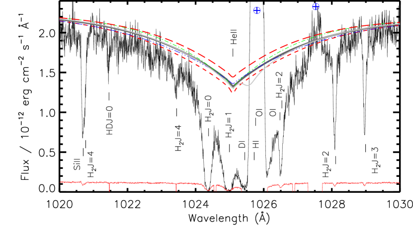
Figure 2: The grid of stellar models described in § 4.1, shifted by radial velocity $v=-52$ km s^-1 and plotted against the LiF1A data and $1\sigma$ errors around H I Ly$\beta$. Thick (dark grey) solid line: $T=115000$ K, $\log g=7.5$, He-dominated (reference model). Thick (red) dashed lines: $T=103500$ K, $\log g=7.5$, He-dominated (lower) and $T=126500$ K, $\log g=7.5$ (upper). Thin (green) dash-dotted line: $T=115000$ K, $\log g=7.2$, He-dominated. Thin (blue) dash-triple dotted line: $T=115000$ K, $\log g=7.8$, He-dominated. Thin (light grey) solid line: $T=115000$ K, $\log g=7.5$, [H/He]=0.2, [C/H]$=5\times 10^{-5}$, [N/H]$=10^{-3}$ and [O/H]$=5\times 10^{-5}$. $\bigoplus$: Geo-coronal Ly$\beta$, O I$\lambda\,1027.5$ emission. ISM and photospheric absorption lines are noted with ticks and labelled. The feature at 1022.7 Å is not in the LiF2B data and appears to be noise.

For the purposes of fitting a stellar continuum to the data, the stellar radial velocity is estimated to be $-52$ km s^-1, based on O VI photospheric absorption lines. We then fitted the model spectra described above to the FUSE data, using separate flux normalizations for each of the eight FUSE detector/channel segments. The models are shown for the Ly$\beta$ region in Fig. 2.

The stellar models were used as a first attempt at a continuum fit for absorption line analysis, except for LiF1B, which had to have a continuum fitted by hand due to the “worm” feature (Sahnow et al., 2000), an optical anomaly due to the astigmatism in the system and a wire mesh in front of the detector. The stellar models were finally given a minor linear correction, determined by eye, to match the flux level in each channel segment. Further local zero-point corrections to the continuum will be allowed in the subsequent analysis. We see no indication of scattered light.

4.2 Methods of line analysis

Curve of growth: The COG technique is often used with FUSE data because it offers an independent technique to determine column densities and Doppler parameters for species with many different oscillator strengths, such as H₂. See Oliveira et al. (2003) for details.

Apparent optical depth: In the AOD technique, the column density is determined by directly integrating the apparent column density profile over the velocity range of the absorption profile. See Savage & Sembach (1991) and Sembach & Savage (1992) for details. We use the AOD technique as a consistency check of the results obtained with PF and COG, and to determine lower limits on the column densities of species which only have saturated transitions in the $FUSE$ bandpass.

Profile fitting: If there are several components contributing to a given atomic transition, profile fitting in principle yields much more information than simple curve of growth analyses. However, the FUSE resolution of $15-20$ km s^-1 is not high enough to resolve typical ISM lines, which generally arise from a number of narrow components over a small velocity interval. H I lines are particularly challenging, in that their intrinsic widths are high due to their low atomic mass. Nevertheless, for blended complexes of lines, one can obtain reasonably accurate estimates for total column density (with a corresponding inflated composite Doppler parameter), provided that the distribution of intrinsic component optical depths and Doppler parameters is smooth (Jenkins, 1986). We employ two profile fitting programs for this work: Owens and vpfit. Owens was developed by M. Lemoine and the French FUSE team at the Institut d’Astrophysique de Paris, and has been used for a number of D/H studies of Galactic targets involving FUSE data. See Lemoine et al. (2002); Hébrard et al. (2002); Hébrard & Moos (2003); Oliveira et al. (2003) for a fuller description. vpfit has been used for many years, but its contribution to D/H work has so far concentrated on extragalactic sight lines (e.g. Webb, 1991; Carswell et al., 1996; Pettini & Bowen, 2001; Crighton et al., 2003). We use both codes here as a check for the robustness of results between the two.

vpfit originally was developed for the analysis of ground-based echelle spectroscopy, but has also been used on various high resolution HST spectra. It generally works best with well-defined wavelength solutions, line spread functions and error arrays, which can be a challenge for FUSE data, and normally is not used to work with as many fitting windows as Owens. vpfit also requires more steps than Owens to deconvolve the effects of turbulent and thermal velocity. Nevertheless, vpfit is easily adaptable and well-supported. Its strength is that it can easily accommodate highly blended complexes, and can generate a $\chi^{2}$ grid relatively quickly compared to Owens. For vpfit results, our errors are calculated based on $\Delta\chi^{2}=\chi^{2}_{min}+1$ for $1\sigma$ and $\Delta\chi^{2}=\chi^{2}_{min}+4$ for $2\sigma$. Like Owens, vpfit can allow a wavelength offset for each fitting region to accommodate uncertainties in the dispersion solution. Similarly, vpfit can permit variations in continuum level. We leave such variations as zero point offsets in those windows which require them, because it is unlikely (and not desirable) that the continuum slope depart significantly from that of the stellar model over the short range (on the order of ${\lesssim}1$ Å) of each fitting window. The reliance of vpfit on a pre-determined continuum with zeroth order adjustments is one of its main differences from Owens, which uses polynomial approximations to model flips and dips in the local continuum and, if desired, to approximate absorption line wings. We employ vpfit as a check for general Owens results and the binning used in its analysis, and typically use vpfit to solve for column densities and Doppler parameters for one or a small number of species at a time. For this reason, we generally leave the Doppler parameter free to vary by species, with the benefit that unphysical Doppler parameters may signal that the LSF or blended component structure may be poorly understood in a fitting region.

For the vpfit analysis, the data were left unbinned, to permit the exclusion of the narrowest intervals which are suspected noise spikes and regions contaminated by airglow. For the AOD, COG and Owens analyses in this paper, the data were chosen to be binned by three pixels to increase the signal to noise ratio, as allowed by the oversampling of the LSF. For the vpfit analysis, we use negative $\sigma$ values as flags to omit data from profile fits, whereas for Owens, bad data were flagged by high $\sigma$ values. Wavelength ranges for measurement intervals for the COG, AOD and the two PF methods were not required to be the same.

All three methods described above provide formal statistical error estimates. Systematic errors, which were discussed in detail by Hébrard et al. (2002), also have an important effect in overall error estimates, and will also be considered in this study.

4.3 Na I Optical Data

The Keck spectra of the Na I 5891,5897 lines are shown in Fig. 3. We used the PF and AOD techniques to determine the column density of Na I. Following the procedure outlined in Sembach & Savage (1992), we find equivalent widths W_λ($\lambda$5891) = 173.72 $\pm$ 5.62 mÅ, and W_λ($\lambda$5897) = 107.71 $\pm$ 4.00 mÅ.

4.3.1 Profile Fitting

Profile fitting of the Na I doublet with Owens was performed independently of the other atomic species, with one and two absorption components. The column densities derived with one and two components are consistent with each other: $\log N(\mbox{{Na~{}I}})=12.19\pm 0.04$ ($2\sigma$). The fits are shown in the bottom panels of Fig. 3. Using two components does not significantly improve the quality of the fit determined from the $\chi^{2}$ statistic, leading us to conclude that at the Keck spectrum’s resolution of 8.3 km s^-1 the Na I lines are consistent with a single absorption component centered at $v\sim-$6 km s^-1. (Radial velocities are given in the heliocentric frame). vpfit gave a satisfactory fit for a single component at $v=-5.1\pm 0.3$ km s^-1, with Doppler parameter $3.6^{+0.4}_{-0.2}$ km s^-1  and $\log N(\mbox{{Na~{}I}})=12.25\pm 0.04$ ($2\sigma$ errors). We adopt $v=-5.1$ km s^-1 as an absolute velocity reference for the neutral gas in the FUSE data. We note that Na I is an imperfect tracer of H I (Cha et al., 2000), but have no other high resolution information for the ISM absorption velocity structure.

4.3.2 Apparent Optical Depth

The top panel of Fig. 3 compares the apparent column density of the two components of the Na I doublet as a function of velocity. The two profiles are not consistent in the range $-12<v<-$1 km s^-1, indicating that there is some unresolved saturated structure at these velocities. Disagreements between the two profiles for $v<-20$ km s^-1 and $v>+4$ km s^-1 are at the level of noise in these regions. We derive apparent column densities, $\log N(\mbox{{Na~{}I}})=12.15\pm 0.02$ for the weaker line (5897.56 Å) and $\log N(\mbox{{Na~{}I}})=12.11\pm 0.02$ for the stronger line (5891.58 Å). Since the difference between the log of the two apparent column densities is less than 0.05 dex, we can use the procedure outlined by Savage & Sembach (1991) to correct for the small saturation effects in these transitions. A better estimate of the true column density is then achieved with $\log N_{a}=\log N(\mbox{{Na~{}I}})_{\lambda 5897}+\Delta\log N(\mbox{{Na~{}I}})_{\lambda 5891-5897}$, where the first term in the equation is the column density derived from the weaker member of the doublet (Na I 5897 Å) and the second term corresponds to the difference in column density derived from the two lines of the doublet. Using the equation above we obtain $\log N(\mbox{{Na~{}I}})=12.19\pm 0.04$ ($1\sigma$), consistent with the profile fitting results and which we adopt.

4.4 Molecular hydrogen

The PG 0038$+$199 FUSE data have a rich H₂ absorption spectrum, and many of the H₂ features are saturated and/or blended. It is crucial, however, to have a good constraint on the various H₂ transitions, because the lines are often blended with D I, H I and all other atomic ISM species. We used both curve-of-growth and profile fitting methods to constrain $N(\mbox{H${}_{2}$})$.

4.4.1 Curve of Growth

For the COG method it was assumed that a single Doppler parameter, $b$, describes all the rotational levels of H₂ and HD. For both of these molecules, equivalent widths corresponding to a total of 91 different transitions (6, 7, 33, 25, and 14 for the $J=0,1,2,3,4$ rotational levels of H₂ respectively; 6 for HD $J$ = 0) were measured in all the FUSE channels where they are detected (Table 2). We did not use $J=5$ for a COG analysis because it is too weak. The equivalent widths for each line, measured in different detector/channel segments, were then compared. All of them agree within the 2$\sigma$ errors, though we regard the results for $J=0$ and 1 with caution due to blending. These equivalent widths were then combined through a weighted average, and a single-component COG was fitted to the 91 values. It is shown in Figure 4. The COG fit yields $b=3.1^{+0.3}_{-0.2}$ km s^-1.

4.4.2 Profile Fitting

For profile fitting with Owens, CO used a single Gaussian line spread function (LSF) to describe the instrumental line spread function, with a full width FWHM of 10.5 unbinned pixels. GH allowed the LSF to vary. Hébrard et al. (2002) found from Owens profile fits for D/H work that $\Delta\chi^{2}=4$ (or $2^{2}$) at the $2\sigma$ level for errors in line fitting parameters such as column density, $\Delta\chi^{2}=9$ (or $3^{2}$) for $3\sigma$, and similarly up to $7\sigma$. This $\Delta\chi^{2}=k^{2}$ for $k\sigma$ relation is used in our Owens analysis to establish $2\sigma$ errors based on averages from 1$\sigma$ to 7$\sigma$. The profile fitting of the H₂ and HD lines was performed simultaneously with the other atomic species for which the column densities were being sought. We used 11, 18, 12, 8, 18, 14 lines for the $J=0,1,2,3,4,5$ H₂ rotational levels in all the FUSE channel segments where they were seen. H₂ and HD were not restricted in radial velocity in comparison to atomic species nor, in the case of the analysis of GH, to each other, who found a radial velocity difference $|v_{\mathrm{H}_{2}}-v_{\mathrm{H}D}|=4.6$ km s^-1 using this approach. We derive $b_{\mathrm{H}_{2},HD}\sim 2.7$ km s^-1.

vpfit is less well-suited than Owens for fitting simultaneously the very large number of spectral regions containing H₂ and HD lines in the PG 0038$+$199 data. We therefore used it to determine the wavelength-dependent LSF, based on H₂ column densities and Doppler parameters from the COG and Owens results (Appendix B). It is then possible to offer a consistency check and estimate of the profile fitting uncertainties with vpfit, using a subsample of fitting regions from the LiF1A segment. We made trial fits fixing the Doppler parameter at $b=2.7$, 3.1, 3.4 km s^-1 based on the PF and COG estimates, and took the range of H₂ column densities as a function of $b$ for the various rotational levels as roughly $2\sigma$ systematic errors. The range in values from the COG and Owens PF measurements were also treated as $2\sigma$ contributions to the systematic error. We then compared the $2\sigma$ statistical errors for the various PF and COG methods, and the variations in column density as a function of Doppler parameter and the variations in column density between the various PF and COG methods as approximate $2\sigma$ errors in the approach taken by Wood et al. (2004), to form overall $2\sigma$ estimates in the H₂ and HD column densities. The exact H₂ column densities do not make a significant difference to atomic column densities except in the case of H I (§ 4.6).

H₂ and HD column densities are presented in Table 3. The quoted uncertainties are $2\sigma$. Discrepancies in the COG and PF results make $1\sigma$ uncertainties difficult to estimate, but we assume that $1\sigma$ errors would be roughly half the $2\sigma$ errors. The total H₂ column density along this line of sight is $\log{\mathrm{N}}(\mbox{H${}_{2}$})=19.33\pm 0.04$ ($2\sigma$), and $\log({\mathrm{HD}}/\mbox{H${}_{2}$})=-5.38^{+0.06}_{-0.05}$ ($2\sigma$). Column density results were insensitive to the exact LSF used.

To estimate the H₂ excitation temperature, we fitted the $J=0$ and 1 levels independently of the other levels, and find $T_{\rm 01}=136\pm 21$ K. The column densities for the various $J$ levels divided by their relative statistical weights are shown in Fig. 5. We can also fit the H₂ $0<J<4$ and HD $J=0$ column densities with a single temperature, $T_{\rm 04}=143\pm 5$ K. We note that the $0<J<4$ levels are not usually consistent with a single temperature, and that $T\sim 140$ K is unusually high for Galactic H₂ (Black & Dalgarno, 1973; Snow et al., 2000; Rachford et al., 2001, 2002). Using the H I column density derived in § 4.6, we compute the fraction of H₂ along the sight line, $f(\mbox{H${}_{2}$})=2N(\mbox{H${}_{2}$})/(N(\mbox{{H~{}I}})+2N(\mbox{H${}_{2}$}))=0.14\pm 0.02$ ($2\sigma$ errors).

Finally, we checked the accuracy of our continuum placement by examining 33 HD lines in the six FUSE segments covering 915-1100 Å. The HD lines are optically thin, and therefore quite sensitive to continuum level. vpfit can calculate zero point continuum correction factors for each of the 33 fitting windows. A simultaneous fit to the HD lines yields an average correction factor of $\langle{\rm cont}\rangle=0.967\pm 0.044$. The continuum we use is thus not systematically low or high, and adjustments have a scatter of $\sim$4%.

4.5 Column Densities of Metal Species

The column densities presented in this work for the atomic species were determined with the PF, AOD and COG techniques. Wavelengths and $f\lambda$ values (and equivalent widths for Fe II) of the metal, H I and D I transitions used in this work are listed in Table 4. In some cases, it was only possible to quote a lower limit via the AOD method for column densities due to saturated transitions in the FUSE bandpass. The COG was used only with Fe II, because this species is the only one which has enough non-saturated and non-blended transitions sufficient for this method.

We included in our model fit for metal lines a molecular cloud with H₂ and HD, as described in § 4.4, because many atomic transitions are blended with H₂. The C I absorption will follow cool gas like that responsible for the H₂ and Na I absorption rather than the warm gas that will be responsible for much of the H I, D I, N I and O I absorption. Therefore, for Owens PF results, for co-author CO, D I, N I, O I and Fe II were fitted in one component, and C I and H₂ in another. Co-author GH did not include C I in his fits. Atomic column densities are listed in Table 5.

An example fit to O I $\lambda 974$, which is the only available unsaturated O I line and the entire basis of our O I column density measurement, is in Fig. 6. It is strongly blended with H₂ $J=2$ and 5. The resolution in SiC2A at 974 Å is $\sim 18$ km s^-1, which is among the best in our data. However, in SiC1B it is $\sim 30$ km s^-1, among the worst. The SiC2A data therefore provide the strongest constraints. Co-author GH only used the SiC2A data for his Owens fit, while co-authors CO and GW also included the SiC1B data for their Owens and vpfit (see below) calculations, respectively. All three co-authors found consistent results with each other. We regard $N(\mbox{{O~{}I}})$ with caution, because of its dependence on one line with good resolution only in the SiC2A data. We will discuss $N(\mbox{{O~{}I}})$ further in § 5.1.

For vpfit PF results, we used the wavelength-dependent LSF derived in Appendix B, and fitted each species independently. The Doppler parameters were left free to vary, as a check for LSF problems or evidence of substantial unresolved blending. A significant ($>2\sigma$) difference between vpfit and Owens results only arose for N I, for which the best fit Doppler parameter would require $b=9.0^{+1.1}_{-0.5}$ km s^-1, which is high compared to $b$ from H₂. If we fix the Doppler parameter to $b_{\mathrm{NI}}=3.1$ km s^-1 (based on the value from H₂), then we obtain $N(\mbox{{N~{}I}})$ from vpfit, consistent with the fits from both co-authors who used Owens. However, despite the simplicity of the Na I absorption, it is likely that the H I, O I and N I absorption (which will be from warm as well as cold gas) will have multiple components, in which case $b=9.0$ km s^-1 is not unreasonably high but is simply a consequence of the unresolved velocity structure. Likewise, assuming the $b$ value from the H₂ fit for N I may be completely inappropriate since to a large extent the H₂ and N I absorption may be coming from entirely different places.

Otherwise, the results are consistent between the one vpfit and two Owens calculations, and in particular are independent of how C I is included in the fits. The column densities derived for the atomic species are presented in Table 5, and are a compromise of Owens and vpfit values. We also found a number of unidentified lines, listed in Table 6, which may be either stellar or interstellar.

4.6 H I and D I Column Densities

The Ly$\alpha$ transition provides the best determination of $N(\mbox{{H~{}I}})$ for the highest column densities, based on damping wings. Unfortunately, only IUE low resolution data cover the Ly$\alpha$ region for PG 0038$+$199, and the ISM Ly$\alpha$ trough is filled in, presumably by geo-coronal emission. FUSE provides wavelength coverage from the Lyman limit up to Ly$\beta$. We must therefore make an estimate of H I column density based on Ly$\beta$, which is blended with a large number of H₂ and O I transitions, but which offers promise due to strong damping wings.

4.6.1 H I and D I column densities

H I: For the Owens calculations, we fitted the Ly$\beta$ profile separately from the other species. However, because H I and D I are blended with O I and H₂, we used the column densities of the latter, determined in § 4.4.2–4.5, as fixed constraints. All four of the H I Ly$\beta$ profiles obtained with the LiF and SiC channels were used simultaneously. The two LiF channels dominate the results because of their higher signal to noise ratio.

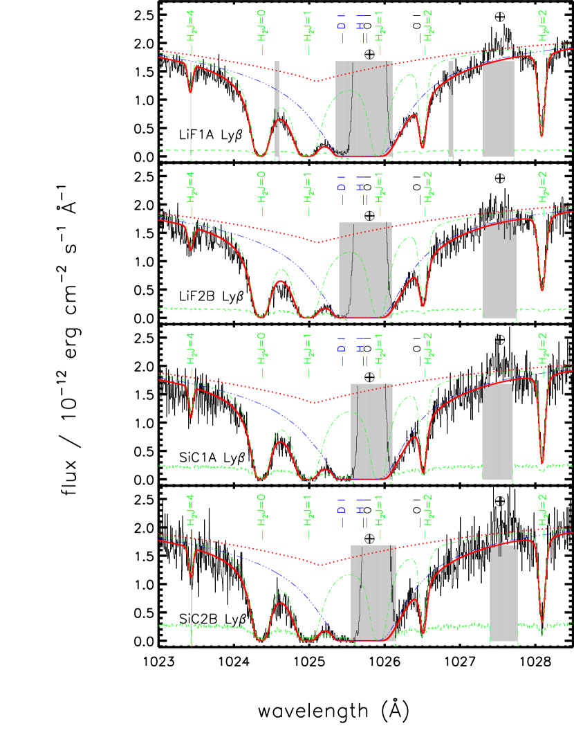
Figure 7: Solid (red) line: vpfit combined fit to H I, D I, O I and H₂. Dashed (green) line: $1\sigma$ error array. Dash-dotted (green) line: H₂ profiles (all lines shown after convolution with local LSF). Dash-triple-dotted (blue) line: HI, DI profiles. Dotted (red) line: Stellar continuum. O I profiles are not shown because they fall in geo-coronal Ly$\beta$ emission and are dominated by H₂ lines. $\bigoplus$: Geo-coronal Ly$\beta$, O I$\lambda\,1027.5$ emission. Grey zones: regions which were excluded from the fit, including geo-coronal emission and noise spikes. H₂, H I, D I and O I transitions are marked by ticks.

The vpfit analysis of the H I column density included a simultaneous fit to all segments covering Ly$\beta$, Ly7, Ly8, Ly9 and Ly10. However only Ly$\beta$ determines the column density, with the profile fit shown in Fig. 7. The higher order lines were included in the fit for consistency and to constrain the Doppler parameter, as will be discussed below. We did not include Ly$\gamma$, $\delta$, $\epsilon$ and Ly-6 in the fits because they do not present strong enough damping wings to constrain the H I column density, and are too saturated to constrain the D I column density. As a check, we did obtain a statistically consistent fit for our adopted results (see below) for Ly$\gamma$ and Ly$\delta$ with vpfit, after exercising care in excluding regions affected by geo-coronal emission, which we confirmed by separating our data into day and night subsets. The various H₂ and HD column densities were fixed according to the values in Table 3, which resulted in a best fit of $\log N(\mbox{{H~{}I}})$ = 20.41. Errors will be discussed in the next section. The effective H I Doppler parameter is $13.6\pm 0.2$ km s^-1 ($2\sigma$ errors), which is most likely an inflated value of $b$ due to the presence of unresolved components (Jenkins, 1986).

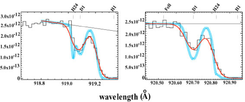
Figure 8: Owens fit to D I Ly9 and Ly10 profiles (SiC2A channel, normalized data, binned by 3 pixels). Red lines: fit after convolution with the local LSF. Thick blue lines: individual components (labelled with ticks), before convolution. Solid black lines: local continua. Flux is in erg cm^-2 s^-1 Å^-1.

D I: With Owens, the D I lines for Ly7, 8, 9, 10 were fitted, and the H I line parameters were also permitted to vary in the fit. For GH, only the SiC2A data were used. A fit from Owens to Lyman 9 and 10 is shown in Fig. 8. The reduced $\chi^{2}$ value is 1.04, with 1442 degrees of freedom. CO included both SiC1B and SiC2A in the calculation, and had $\chi^{2}=1.65$ for 1878 degrees of freedom. Results between the two measurements were consistent, showing that including only the highest resolution data made no significant difference.

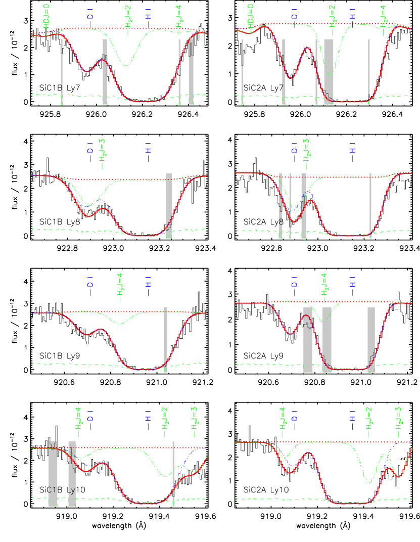
Figure 9: Solid (red) line: vpfit combined fit to H I, D I and H₂ (all profiles shown after convolution with local LSF). Dashed (green) line: $1\sigma$ error array. Dot-dashed (green) line: H₂ profiles. Triple-dot-dashed (blue) line: HI, DI profiles. Dotted (red) line: Stellar continuum. Grey zones: regions which were excluded from the fit, including geo-coronal emission and noise spikes. The thick dashed and solid lines represent the continuum and the fit, respectively. H₂, H I and D I transitions are marked by ticks. Flux is in units of $10^{-12}$ erg cm^-2 s^-1 Å^-1.

With vpfit, the reduced $\chi^{2}$ value is 1.03 for 3635 degrees of freedom over Ly$\beta$,7,8,9,10, shown in Fig. 9. In case the saturated Ly$\beta$ D I line skews the statistics, we also made a fit with only Ly7,8,9,10. Results were not changed significantly.

Comparing the Owens and vpfit results, we agree on a column density $\log N(\mbox{{D~{}I}})=15.75$. Errors are discussed below. The Doppler parameter, assumed to be a composite from several unresolved components as for H I, is $b=11.9\pm 1.6$ km s^-1 ($2\sigma$ errors).

We checked the D I column density using the AOD and COG methods. For the AOD method we find $\log N(\mbox{{D~{}I}})=15.68\pm 0.15$ ($1\sigma$ error in the mean). A COG study for the SiC2A data (which have higher resolution than SiC1B) yields $\log N(\mbox{{D~{}I}})=15.80^{+0.07}_{-0.06}$, $b=10.7^{+2.8}_{-1.8}$ km s^-1. These values are consistent with our PF results.

4.6.2 H I and D I Column density errors

Hébrard et al. (2002) identified and discussed a number of systematic effects which can affect column density estimates. Following their example, we considered the potential systematic effects from the following sources:

Continuum uncertainty: Both vpfit and Owens can explicitly include local normalization corrections in their calculations of statistical uncertainties.

For the Owens analyses, the local continuum is free to vary for each spectral window, and is approximated by a polynomial of order $\sim 2-4$. Uncertainties from the continuum approximation are reflected in the $\chi^{2}$ statistics (e.g. Hébrard et al., 2002; Oliveira et al., 2003).

For the vpfit analysis, we allowed the continuum for each stellar model to have a zeroth order correction factor in each of the 12 fitting regions (4 for Ly$\beta$ and 2 each for Ly7, 8, 9, 10), with a mean value of $0.963\pm 0.041$ ($1\sigma$). The correction factor is thus (just) consistent with unity, and is consistent with the continuum uncertainty from HD (§ 4.4.2). We note that the multiplicative corrections for the four Ly$\beta$ regions are $0.974\pm 0.004$, $0.930\pm 0.005$, $0.936\pm 0.006$ and $0.936\pm 0.007$ for the LiF1A, LiF2B, SiC1A and SiC2B segments respectively, which may indicate a local systematic overestimation of the stellar model flux. Continuum differences between the models throughout the data except in the Ly$\beta$ region are ${\lesssim}4-5$% (§ 4.1), and are thus consistent with the local continuum variations in the Ly$\beta$ region for our profile fits. Continuum differences in the Ly$\beta$ region are discussed below. The stellar model including [He/H]=5 and metals produced smaller continuum normalization corrections at H I $\lambda 923$ and D I $\lambda 922$, because it included contributions from N IV. However, the model with metals did not produce a statistically acceptable overall fit in the Ly$\beta$ region, in contrast to the metal-free models. In any case, the inclusion of metals in the stellar model had no significant effect on either H I or D I column densities.
Stellar model: We compare results for the grid of stellar models described in § 4.1. The maximum deviation between the best fit and other models is $\pm 10$% . This occurs for the He-rich, metal-free models over $1025.2-1025.4$ Å (He II $\lambda 1025$), or for the model with [He/H]=5 and metals at Ly$\beta$. Typical deviations in the damping wings are on the order of $\leq 5$%. For the Owens analysis, the Ly$\beta$ region was fitted using the stellar model grid without allowing for continuum corrections, producing a systematic error of $\sim\pm 0.05$ dex ($2\sigma$). For the vpfit analysis, a similar calculation employing local continuum zeroth order corrections resulted in variations in column density of $\Delta\log N(\mbox{{H~{}I}})=0.02$ and $\Delta\log N(\mbox{{D~{}I}})=0.002$ ($2\sigma$).
Line spread function: We varied the LSF by 2 km s^-1 ($\sim 1\sigma$), which produced changes of $\Delta\log N(\mbox{{H~{}I}})=0.005$ and $\Delta\log N(\mbox{{D~{}I}})<0.001$. These differences are both significantly smaller than the statistical errors (see below). We do not consider LSF uncertainties further in our source of error.
H₂ column densities: We varied the H₂ column densities, trying the COG and PF results for $\log N(\mbox{H${}_{2}$})$ for the ensemble of $J=$0,1,2,3,4,5 and HD as rough $2\sigma$ upper and lower $\log N(\mbox{H${}_{2}$})$ bounds, respectively. The resulting column density variations are $\Delta\log N(\mbox{{H~{}I}})=0.03$ and $\Delta\log N(\mbox{{D~{}I}})=0.01$ ($\sim 2\sigma$). H₂ column density uncertainty is a major systematic error for our H I and D I column densities.

A $\chi^{2}$ grid in $\log N(\mbox{{H~{}I}})$, $\log N(\mbox{{D~{}I}})$ gives statistical errors of $\Delta\log N(\mbox{{H~{}I}})=0.02$ and $\Delta\log N(\mbox{{D~{}I}})=0.04$ (both $2\sigma$). Combining the systematic and statistical errors in quadrature yields $\log N(\mbox{{H~{}I}})=20.41\pm 0.08$ and $\log N(\mbox{{D~{}I}})=15.75\pm 0.08$ ($2\sigma$).

We are encouraged that the results are so similar between the Owens and vpfit analyses by three different people, and including four independent FUSE measurements. Furthermore, the results are robust, despite the use of binned vs. unbinned data, the variation of continua, stellar models, LSF and H₂ column densities. This line of sight is only the third D/H target for which only FUSE data are used to determine $N$(H I), the first two being from Wood et al. (2004).

4.6.3 Other estimates for H I column density

The total H column density, $\log N(\mbox{{H~{}I}}+2\mbox{H${}_{2}$})$, defined here as H_T, is $20.48\pm 0.07$ ($2\sigma$), which is in accord with that predicted using Na I (Ferlet, Vidal-Madjar & Gry, 1985). They employed 78 stellar sight lines to determine $\log N(\mbox{{Na~{}I}})=1.04[\log N(\mbox{{H~{}I}}+\mbox{H${}_{2}$})]-9.09$ (their equation 1), with a correlation coefficient of 0.85 and slope of $1.04\pm 0.08$. Using our measured column density of $\log N(\mbox{{Na~{}I}})=12.19\pm 0.04$ ($2\sigma$) yields $\log N(\mbox{H${}_{T}$})=20.46^{+1.75}_{-1.42}$, with the uncertainty dictated by the slope error in the Ferlet, Vidal-Madjar & Gry relation. The color excess $E(B-V)=0.037$ offers a prediction of $\log N(\mbox{H${}_{T}$})=20.3$ with a scatter of $\sim 50$% (Savage & Mathis, 1979).

We also examined the H I 21 cm profile from the Leiden-Dwingeloo H I survey (Hartmann & Burton, 1997), and find $\log N(\mbox{{H~{}I}})=20.36$. This result is for a velocity resolution 1.03 km s^-1, 0.07 K temperature sensitivity and $0.5^{\circ}$ resolution on the sky centered at Galactic coordinates $\ell=120^{\circ}$, $b=-42.5^{\circ}$ (13 arcmin from PG 0038$+$199). See Fig. 10 for a velocity profile of the H I 21 cm flux. We integrated at the position of PG 0038$+$199 between $-20<v<20$ km s^-1 to avoid a secondary peak of emission on the blue side. If we integrate over $-100<v<100$ km s^-1, $\log N(\mbox{{H~{}I}})=20.47$. The beam size is likely large compared to variations in H I, and there is no way to tell from our FUSE data how much H I lies behind PG 0038$+$199, which would increase the column density compared to what we could see in absorption with FUSE. Gas which is far behind PG 0038$+$199 would likely be very far from the disk, given its Galactic latitude. Despite these uncertainties, the closeness of the Leiden-Dwingeloo survey column density to that of our absorption measurement lends supporting evidence to our result, and implies that the H I is not very patchy in this part of the sky. In any case, there is no evidence for a column density as large as $\log N(\mbox{{H~{}I}})=20.57$, which would be necessary to bring the D/H ratio (discussed in the next section) down to the Local Bubble value of $1.5\times 10^{-5}$.

5 Results and Discussion

Combining the results of our column densities for N I and O I with those for D I, H I, HD and H₂, we obtain the relative column density ratios as listed in Table 7 and shown in Fig. 11. We consider the ratios between the column densities for D I, H I, O I, N I each in turn, beginning with ratios relative to hydrogen, and compare our results to those in the literature. If we include H₂ and HD contributions, we find $\log[N(\mbox{H${}_{T}$})]=20.48\pm 0.07$ ($2\sigma$), and $\log[N(\mbox{{D~{}I}})+N({\mathrm{HD}})]=15.76\pm 0.08$ ($2\sigma$). We therefore quote various ratios including H₂ and HD, as well as the traditional form D/H, plus the HD/H₂ ratio. We approximate $1\sigma$ errors for HD and H₂ as half the $2\sigma$ errors for contributions to [D I + HD]/[H I + 2H₂], O/[H+2H₂] and N/[H+2H₂]. We neglect HD for the total H contribution since (HD/[H I+2H₂] $<10^{-6}$).

5.1 Column density ratios

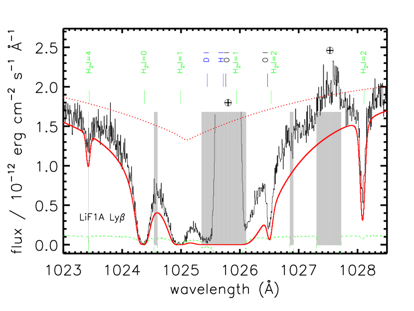
Figure 13: A model curve for $\log N(\mbox{{H~{}I}})=20.83$ plotted with the LiF1A data, which would be necessary to bring D/H=$0.85\times 10^{-5}$, in accord with other high H I column density sight lines. Such a high column density is firmly excluded by the data. Line styles and symbols are as in Fig. 7. Column densities for D I, O I and H₂ have been kept constant at their best-fit values.

[D I + HD]/[H I + 2H₂]: We obtain a value of $(1.91^{+0.52}_{-0.42})\times 10^{-5}$ ($2\sigma$ errors), shown in Fig. 12, which is significantly high compared to $\mbox{\rm D/H}=(0.85\pm 0.09)\times 10^{-5}$ for sight lines with $\log N(\mbox{{H~{}I}})\geq 20.5$ and distances $d>500$ pc (Wood et al., 2004). The possibility of a low D/H value toward distant sight lines was first proposed by Hébrard & Moos (2003), based on D/O and D/N measurements, and previously published D/H values. Wood et al. corroborated the argument, compiling a large set of D/H measurements from the literature (though only four were for $\log N(\mbox{{H~{}I}})>20.5$). If we exclude the molecular component, $\mbox{\rm D/H}=(2.19^{+0.65}_{-0.50})\times 10^{-5}$ ($2\sigma$ errors) making an even greater discrepancy with similar H I column density sight lines. We believe that our [D I + HD]/[H I + 2H₂] and D/H ratios for PG 0038$+$199 are robust, based on measurements from three individuals using two different software packages and allowing for a variety of systematic errors. Our largest source of uncertainty is systematic errors in the H I column density, because we do not have access to Ly$\alpha$. We would require $\log N(\mbox{{H~{}I}}+\mbox{H${}_{2}$})=20.83$ to have $\mbox{\rm[\mbox{{D~{}I}}\ + HD]/[\mbox{{H~{}I}}\ + 2\mbox{H${}_{2}$}]}=0.85$, which is many $\sigma$ from our result. Such a high value makes a poor fit to the data, and is shown in Fig. 13.

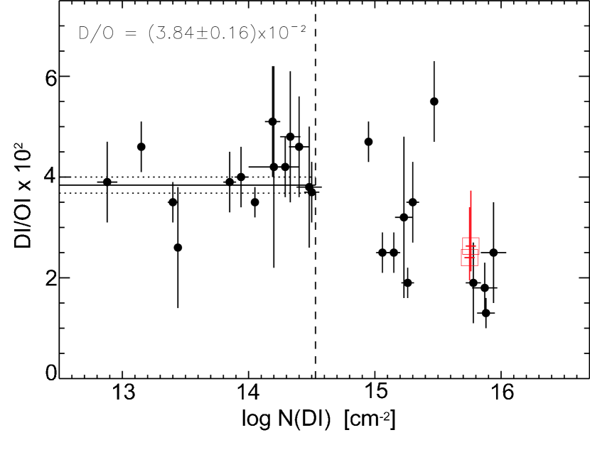
Figure 14: DO vs. $\log N(\mbox{{D~{}I}})$ for a number of sight lines, with $1\sigma$ error bars, as in Hébrard & Moos (2003) and including values from Wood et al. (2004). Values for PG 0038$+$199 (both including and excluding HD contributions) are indicated by open boxes. The dotted line indicates the limit inside the Local Bubble, inside which the D/O ratio is homogeneous.

[D I + HD]/O I: Our result is $(2.63^{+2.18}_{-0.85})\times 10^{-2}$ ($2\sigma$). If the HD contribution is excluded, the ratio drops to: $\mbox{\rm D/O}=(2.40^{+2.19}_{-0.78})\times 10^{-2}$ ($2\sigma$). For the sample $\log N(\mbox{{D~{}I}})>15.5$ and distance $d>300$ pc, our values are within the Hébrard & Moos range for $(1.5{\lesssim}\mbox{\rm D/O}{\lesssim}2.5)\times 10^{-2}$, shown in Fig. 14, though we note that there are only three values with that D I column density threshold in their sample. The $N(\mbox{{O~{}I}})$ error dominates the uncertainty.

O/[H+2H₂]: We regard our O I column density measurement with extreme caution, because it depends entirely on one line at 974 Å strongly blended with two H₂ lines, dominated by the SiC2A data. We compare our results with the O/H determination of Meyer, Jura, & Cardelli (1998), whose sample resembles our sight line in H I column density. Our value of $\mbox{\rm O/[H+2\mbox{H${}_{2}$}]}=(7.76^{+3.38}_{-3.49})\times 10^{-4}$ ($2\sigma$ errors) is $>2\sigma$ higher than the local ISM value of $\mbox{\rm O/H}=(3.43\pm 0.15)\times 10^{-4}$ ($1\sigma$) from Meyer et al. using the updated O I oscillator strength of Welty et al. (1999). If a H I column density error were the sole cause of the O/H discrepancy, we would require $\log N(\mbox{{H~{}I}})=20.82$ to bring O/H to $3.58\times 10^{-4}$, or within the $1\sigma$ error of the revised Meyer, Jura, & Cardelli value. However, such a high value for $N(\mbox{{H~{}I}})$ is highly unlikely, given our determinations from the FUSE data and in light of other $N(\mbox{{H~{}I}})$ estimation methods discussed in § 4.6.3.

Another source of O/H uncertainty depends on the accuracy of the O I 974 Å line oscillator strength, which is theoretically calculated and is estimated to be good to 25% (Biémont & Zeippen, 1992; Wiese, Fuhr & Deters, 1996). In addition to PG 0038$+$199, other objects in the literature for which $N(\mbox{{O~{}I}})$ depends only on O I 974 are JL9, LSS 1274 (Hébrard & Moos, 2003; Wood et al., 2004) and HD 90087 (Hébrard et al., 2004). They, too, exhibit high values of O/H, though the local ISM value lies close to or within their $2\sigma$ formal errors. If the O I 974 oscillator strength were to increase by 15% (0.06 dex), then the nominal O I column density toward PG 0038$+$199 would drop to $\log N(\mbox{{O~{}I}})=17.31$, with O/[H+2H₂] $=6.8\times 10^{-4}$, putting the local ISM value within the $2\sigma$ error for PG 0038$+$199. The nominal D/O value would increase from to $2.40\times 10^{-2}$ to $2.57\times 10^{-2}$, which still lies within the scatter of high column density data points from Hébrard & Moos (2003) (see above). The O I 974 oscillator strength appears consistent with that of O I 1356 in the case of HD 195965 (Hoopes et al., 2003; Hébrard et al., 2004), with the Hoopes et al. (2003) uncertainty in $\log N(\mbox{{O~{}I}})$ being $+0.04,-0.06$ dex – close to the value we require if the discrepant O/H value toward PG 0038$+$199 arises because of an oscillator strength difference. Our D/H and D/O results are consistent with a larger variation in D/H than in D/O (Hébrard & Moos, 2003). However, we find O/H toward PG 0038$+$199 anomalous, because the variations in O/H found by Meyer et al. were small, and we cannot identify a specific reason why the measurement would be in error. If we exclude the H₂ contribution, the O/H discrepancy is even larger: $\mbox{\rm O/H}=(8.51^{+4.09}_{-3.86})\times 10^{-4}$ ($2\sigma$). Observations of additional lines of sight will show whether the combination of D I, H I and O I column densities found toward PG 0038$+$199 produce an outlier, are consistent with other sight lines or are subject to an unidentified error.

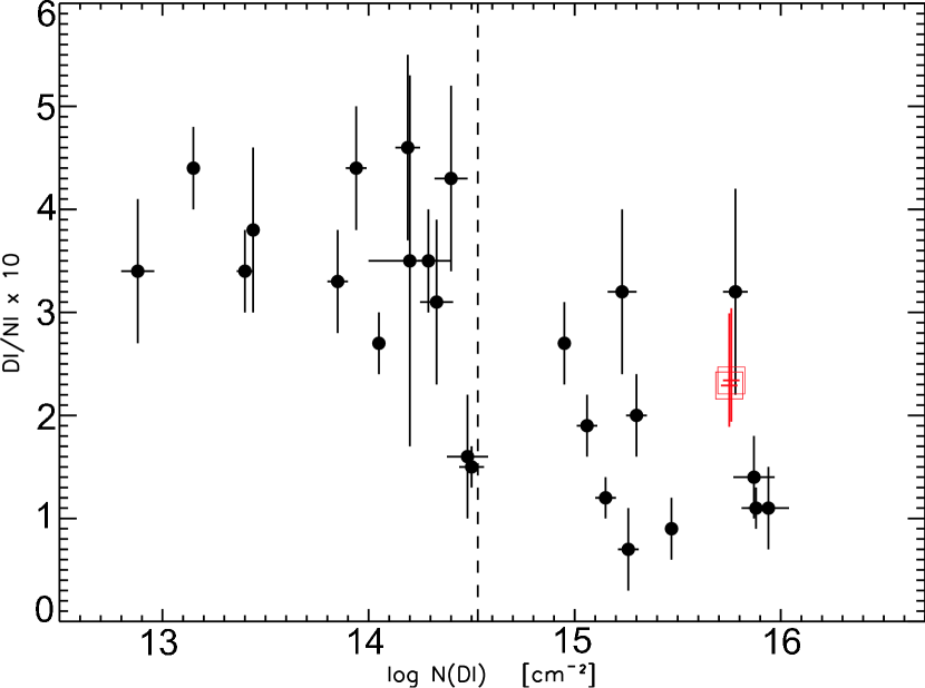
Figure 15: As in Fig. 14, but D/N vs. $\log N(\mbox{{D~{}I}})$.

D/N: We find $\mbox{\rm[\mbox{{D~{}I}}\ + HD]/\mbox{{N~{}I}}}=(2.34^{+1.35}_{-0.72})\times 10^{-1}$ ($2\sigma$), which is high compared to the Hébrard & Moos (2003) values of $(1.0{\lesssim}\mbox{\rm D/N}{\lesssim}1.5)\times 10^{-1}$, shown in Fig. 15, for $\log N(\mbox{{D~{}I}})\geq 15.5$. Omitting the HD fraction results in $\mbox{\rm D/N}=(2.29^{+1.32}_{-0.71})\times 10^{-1}$ ($2\sigma$).

N/[H+2H₂]: We find values of $(0.81^{+0.36}_{-0.29})\times 10^{-4}$ and $\mbox{\rm N/H}=(0.95^{+0.43}_{-0.34})\times 10^{-4}$ (all $2\sigma$), which are consistent within $1\sigma$ errors of the ISM value of $\mbox{\rm N/H}=(0.75\pm 0.04)\times 10^{-4}$ (Meyer, Cardelli, & Sofia, 1997).

N/O: Our value of $\mbox{\rm N/O}=(1.12^{+1.05}_{-0.47})\times 10^{-1}$ ($2\sigma$) is low compared to the ratio $(2.35\pm 0.15)\times 10^{-1}$ for N/H and O/H in the ISM from Meyer, Cardelli, & Sofia (1997) and Meyer, Jura, & Cardelli (1998), due to the high O/H ratio we find. See the discussion above about the reliability of the O I measurement.

HD/2H₂: The deuterium fraction in molecular form is $(2.08^{+0.34}_{-0.25})\times 10^{-6}$ ($2\sigma$ errors), and the column density ratio is HD/H₂ $=(4.17^{+0.68}_{-0.49})\times 10^{-6}$ ($2\sigma$). The HD and H₂ column densities place it within the range of measurements at similar $N(\mbox{H${}_{2}$})$ from Spitzer, Cochran, & Hirschfeld (1974) and Savage et al. (1977), a factor of $\sim 3$ above the expected ratio from charge exchange reactions between H and D (Liszt, 2003), but consistent with the scatter in values.

5.2 Comparison with other high D/H lines of sight

There are only two other noteworthy detections of $\mbox{\rm D/H}\geq 2.1\times 10^{-5}$: $\gamma^{2}$ Vel (Sonneborn et al., 2000) and Feige 110 (Friedman et al., 2002). $\gamma^{2}$ Vel exhibits both high and low ionization absorbers in a 7-member complex (3 H II, 4 H I). Its H I absorption spans a velocity interval of $\Delta v=32$ km s^-1, with a very low H₂ fraction of $1.4\times 10^{-5}$, and $\log N(\mbox{{H~{}I}})=19.71\pm 0.03$ ($1\sigma$ errors), $N(\mbox{{D~{}I}})=(1.12^{+0.15}_{-0.12})\times 10^{15}$ (90% confidence limits) and $\mbox{\rm D/N}=(2.7\pm 0.4)\times 10^{-1}$ at 90% confidence or $1.65\sigma$ significance (Cha et al., 2000; Fitzpatrick & Spitzer, 1994). Although the D/N ratios are consistent within the errors for $\gamma^{2}$ Vel and PG 0038$+$199, in contrast, PG 0038$+$199 does not exhibit numerous high ionization species (though it does show S III), and has a much higher H₂ fraction and H I column density. We cannot compare D/O because the O I column density is difficult to measure for both $\gamma^{2}$ Vel and PG 0038$+$199. Feige 110 has only a slightly smaller H I column density than PG 0038$+$199 ($\log N(\mbox{{H~{}I}})=20.14^{+0.13}_{-0.20}$, $2\sigma$ errors), and $\mbox{\rm D/H}=(2.14\pm 0.82)\times 10^{-5}$ ($2\sigma$). It is possible that PG 0038$+$199 is slightly higher out of the Galactic plane, and is sampling richer, infalling gas, one of several explanations which we consider in the next section.

Another way to characterize the nature of the PG 0038$+$199 sight line versus the $\gamma^{2}$ Vel sight line is in terms of the iron abundance. Jenkins, Savage, & Spitzer (1986) have examined the iron abundances determined from N(Fe II) measured by Copernicus as a function of the average density $\langle N_{H}\rangle$. $\langle N_{H}\rangle$ is defined as $N({\mathrm{H}})=N(\mbox{{H~{}I}})+2N(\mbox{H${}_{2}$})$ divided by the distance to the star. For PG 0038$+$199, $\mbox{$\langle N_{H}\rangle$}=0.3^{+0.2}_{-0.1}$ cm^-3 ($1\sigma$) and the relative iron abundance assumed to be $\log(N(\mbox{{Fe~{}II}})/N({\mathrm{H}}))=-6.06$. This iron abundance is higher than average, but consistent within the uncertainties with the mid-density range results presented by Jenkins and coworkers. On the other hand, $\gamma^{2}$ Vel has an iron abundance more than twice as great as PG 0038$+$199 (Jenkins, Savage, & Spitzer, 1986; Fitzpatrick & Spitzer, 1994) and $\langle N_{H}\rangle$ is much lower, 0.06 cm^-3. In the model discussed by Spitzer (1985) and used by Jenkins, Savage, & Spitzer to analyze the Fe abundance, the two sight lines are quite different. The $\gamma^{2}$ Vel sight line samples only relatively warm diffuse gas with a density of $\sim 0.1$ cm^-3, while the PG 0038$+$199 sight line samples both warm gas and cold higher density fluctuations with a density of $\sim 0.7$ cm^-3 (Spitzer). Jenkins, Savage, & Spitzer assumed that the properties of the grains vary between the two densities and showed by fitting their data set that the relative iron abundance would decrease a factor of four between the extreme cases of only hot gas and only cold gas. However, in this case, although the iron abundance changes by more than a factor of two, as expected, these two sight lines do not show an analagous change in the abundance of deuterium. The values of $\langle N_{H}\rangle$ and the Fe abundances are quite different for PG 0038$+$199 versus $\gamma^{2}$ Vel, indicating that the grain properties along the two sight lines are likely to be different, but there is no evidence for a similar variation in the deuterium abundance.

5.3 Variations in D/H: possible causes

A number of different potential causes for variations in D/H have been discussed in the literature. All causes that have been proposed could produce inhomogeneities in D/H, provided that the ISM mixing time is sufficiently large. Wood et al. (2004) suggested that D/H variations occur on a scale where ISM mixing produces inhomogeneities on scales larger than the Local Bubble, which has a well-established D/H ratio, yet small enough so that the sight lines to the most distant targets investigated for D/H pass through enough inhomogeneous zones for D/H variations to average out to their observed low value of $\approx 8.5\times 10^{-6}$. The strongest challenge to the Wood et al. model would be a sight line with $N(\mbox{{H~{}I}})>20.5$ (or in the Local Bubble) with a high D/H value. PG 0038$+$199 is the highest H I column density sight line with a high D/H value, just below the $\log N(\mbox{{H~{}I}})=20.5$ upper limit for the meso-mixing scale of Wood et al. We now briefly discuss some of the proposed causes of D/H variability below, but see Lemoine et al. (1999) and Draine (2004) for details.

a. Inhomogeneous Galactic infall: Material which has undergone little astration could fall inhomogeneously onto the Galactic disk and produce the observed variation in D/H distribution. One example is from Chiappini, Renda, & Matteucci (2002), which predicts a gradient in D/H as a function of Galactic radius. More data are needed to determine the validity of the model (e.g. Hébrard & Moos, 2003).

b. Astration variations: Variations in the amount of stellar processing experienced by different regions of the ISM could result in D/H variability. An anticorrelation between D/H and O/H has been suggested, on the basis that gas is enriched in O as D is destroyed in stars (e.g. Steigman, 2003). However, the suggestion was tentative because the D/H sample size at the time was noted to be limited. PG 0038$+$199, with its high values of both D/H and (if confirmed) O/H, clearly would be an exception to such an anticorrelation. We share Steigman’s view that more sight lines need to be analyzed to explore the topic further.

c. Variable deuterium depletion: Variations of D/H could be caused by preferential depletion of D onto dust grains relative to H. Draine (2004) noted that such a process could account for the variation in D/H in the ISM while allowing for the relative homogeneity of abundances for N and O. Lipshtat et al. (2004) showed that it is possible for dust to enhance the production rates of HD and D₂ vs. H₂. Observational evidence comes from Peeters et al. (2004), who found infrared spectral evidence of deuterated polycyclic aromatic hydrocarbons (PAHs), and pointed out the large deuterium excess in primitive carbonaceous meteorites and interplanetary dust particles (e.g. Messenger, 2000). Draine also suggested that high velocity shocks could also work in the opposite sense to destroy grains and increase D/H.

Dust depletion processes occur in cold regions of the ISM where H₂ is the dominant reservoir of H. Preferential depletion of D onto dust requires particularly low temperatures (Draine, 2004), so one might expect lines of sight with low H₂ temperatures to have low D/H ratios. Typical ISM H₂ temperatures have been measured to have mean values of $T_{01}\sim 70$ K and rms scatter of $\sim 15$ K for over 80 lines of sight (Savage et al., 1977; Rachford et al., 2002). Wood et al. (2004) noted similar temperatures toward the high H I column density sight lines JL 9 and LSS 1274, and proposed that lines of sight which were recently shocked should have relatively high D/H. H₂ temperatures could be increased in star formation regions, such as near $\alpha$ Cru and $\gamma^{2}$ Vel, the latter being near the Vela supernova remnant. As gas cools, deuterium could be preferentially depleted onto PAHs or grains (Draine, 2004; Peeters et al., 2004; Lipshtat et al., 2004). The H₂ temperature of $T_{01}=136\pm 21$ K toward PG 0038$+$199 is unusually high compared to the mean ISM value, so this is consistent with a high D/H value in the depletion model. Quantitatively, such depletion could reduce D/H by $1\times 10^{-5}$, which is consistent within the errors with the difference in D/H between the PG 0038$+$199 sight line and sight lines with $\log N(\mbox{{H~{}I}})>20.5$.

However, we find no evidence of supernova remnants near PG 0038$+$199 (Stephenson & Green, 2002), nor any sign of nearby anomalous X-ray emission (Snowden et al., 1995) or H$\alpha$ emission (Haffner et al., 2003). The H₂  temperature of PG 0038$+$199 could be raised by the faint remnants of a planetary nebula, though. Two other similarly hot DO stars have H$\alpha$ detections of huge, old, faint PN: PG 0109+111 (Werner et al., 1997, a search which found no old PN around PG 0038$+$199) and PG 1034+001 (Rauch, Kerber, & Pauli, 2004).

If a correlation exists between H₂ temperature and deuterium depletion, it would have to explain sight lines with low D/H and high H₂ rotation temperatures. $\delta$ Ori and $\epsilon$ Ori (Jenkins et al., 2000) exhibit such high rotation temperatures with absorption components having $T_{03}\sim 190-850$ K. (The temperatures for $T_{01}$ are similar to $T_{03}$ for those sight lines. Reasons for the similarity are discussed in Jenkins et al., though we recognize that $T_{01}$ is usually assumed to be the best estimate of the actual thermal temperature.) The H I column densities toward $\delta$ Ori and $\epsilon$ Ori are relatively high ($\log N(\mbox{{H~{}I}})=20.193\pm 0.025$, $\log N(\mbox{{H~{}I}})=20.40\pm 0.08$, $1\sigma$ errors), yet the D/H ratios are low ($0.74^{+0.12}_{-0.09}$, $0.65\pm 0.3\times 10^{-5}$ respectively, $1\sigma$ errors). Their H₂ fractions are low, however ($7\times 10^{-6}$, $1.3\times 10^{-4}$), so a different physical mechanism from that toward PG 0038$+$199 may be at work. In addition, Spitzer, Cochran, & Hirschfeld (1974) found the rotation temperatures of $\gamma^{2}$ Vel and $\zeta$ Pup to be $T_{03}=964\pm 119$ K and $T_{04}=1140\pm 154$ K, (both $1\sigma$) respectively. (Spitzer, Cochran, & Hirschfeld state that their excitation temperatures for $T_{03}$ and $T_{04}$ fit all the observed values of $N(\mbox{H${}_{2}$})$ for the $J$ levels included in the calculation; we estimate $T_{01}$ from their H₂ column densities for $J=0$ and 1 and their equation 1 to be $\sim 300\pm 150$ K and $\sim 350\pm 100$ K respectively, which are still high.) D/H toward $\gamma^{2}$ Vel is high, as discussed in the previous section, but toward $\zeta$ Pup is $(1.42^{+0.25}_{-0.23})\times 10^{-5}$ (90% confidence, Sonneborn et al., 2000), which, given our uncertainties, is marginally below the value for PG 0038$+$199. A larger data set is necessary to investigate the relationship of H₂ temperature and D/H ratio in further detail. Additionally, if this depletion scenario is correct, then D/H may be correlated with the abundance of refractory elements such as Fe. However, as discussed in § 5.2, there is no convincing evidence of such a relationship for PG 0038$+$199.

It is clear that variation in D/H is significant outside of the Local Bubble, and its cause remains an open question. Our understanding of variations in the D/H will improve as theory evolves and further measurements of D/H, H₂ and other ISM species are made at large distances in the Galactic disk and halo.

6 Conclusions

We have observed the He-rich white dwarf PG 0038$+$199 with FUSE and Keck+HIRES and found the following.

1. Keck HIRES data hint at unresolved structure on the order of $\leq 8$ km s^-1 based on Na I.

2. We have compared column densities for a number of ISM species based on a variety of measurements using profile fits from Owens and vpfit, curve-of-growth and apparent optical depth determinations, and found broadly consistent results between the various methods.

3. The H I, D I and H₂ column densities are $\log N(\mbox{{H~{}I}})=20.41\pm 0.08$, $\log N(\mbox{{D~{}I}})=15.75\pm 0.08$, $\log N(\mbox{H${}_{2}$})=19.33\pm 0.04$ with a H₂ fraction $f_{\mbox{H${}_{2}$}}=0.14\pm 0.02$ ($2\sigma$ errors quoted throughout the conclusions, unless otherwise noted). The measurement of $N(\mbox{{H~{}I}})$ for a D/H target is only the third based solely on FUSE data. The H₂ fraction is high enough that we include effects for it and HD in our column density ratios.

4. $\mbox{\rm[\mbox{{D~{}I}}\ + HD]/[\mbox{{H~{}I}}\ + 2\mbox{H${}_{2}$}]}=(1.91^{+0.52}_{-0.42})\times 10^{-5}$ is unusually high for a Galactic value. Variations in D/H outside the Local Bubble are significant. $\mbox{{N~{}I}}/(\mbox{{H~{}I}}+2\mbox{H${}_{2}$})=(0.81^{+0.36}_{-0.29})\times 10^{-5}$ is consistent with the mean ISM value (Meyer, Cardelli, & Sofia, 1997). $\mbox{\rm[\mbox{{D~{}I}}\ + HD]/\mbox{{N~{}I}}}=(2.34^{+1.35}_{-0.72})\times 10^{-1}$ is high for $\log N(\mbox{{D~{}I}})\geq 15.5$ (Hébrard & Moos, 2003, though their sample size is small). $\mbox{\rm O/[H+2\mbox{H${}_{2}$}]}=(7.76^{+3.38}_{-3.49})\times 10^{-4}$ is unusually high, with $\log N(\mbox{{O~{}I}})$ depending on a single line measurement. However, $\mbox{\rm D/O}=(2.40^{+2.19}_{-0.78})\times 10^{-2}$ is consistent with three other distant sight lines (Hébrard & Moos, 2003). Further observations should determine whether the high O/H value remains an anomaly, arises as a result of some uncertainty (e.g. O I 974 oscillator strength) or can in fact be statistically expected.

5. The HD/H₂ ratio is $(4.17^{+0.68}_{-0.49})\times 10^{-6}$, consistent with the scatter of previously measured values for $\log N(\mbox{H${}_{2}$})\approx 19.3$ (Liszt, 2003).

6. A number of mechanisms which produce variation in D/H remain plausible. The H₂ excitation temperature of $143\pm 5$ K ($1\sigma$) may indicate past star formation in the vicinity of PG 0038$+$199, liberating D which may otherwise be depleted onto grains, thereby potentially explaining the high D/H value. However, there are low D/H sight lines with even higher excitation temperatures. More sight lines outside the Local Bubble need to be observed to characterize the D/H distribution and physical processes associated with it.

Appendix A Details on the reduction of $FUSE$ data

We present details on the reduction of FUSE data, as the use of vpfit creates a need for accurate $\sigma$ errors, a desire for the most accurate wavelength calibration possible and requirement for knowledge of the LSF as a function of segment and wavelength.

A.1 Correction of $\sigma$ values

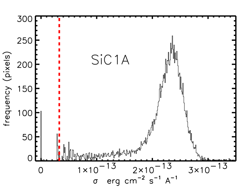
Figure 16: Example distribution of $\sigma$ error values for SiC1A segment. The dotted line shows the point at which we set a floor for $\sigma$ values for SiC1A data.

We established a minimum value for the $\sigma$ array based on the distribution of $\sigma$ values for each segment. Individual pixels with values of $\sigma$ which are unrealistically low make it difficult or impossible to obtain acceptable statistical results for profile fitting. The mean flux and signal to noise ratio per pixel for the eight segments before modification of the $\sigma$ values, for $\lambda>915$ Å and where $\sigma>0$, ranges over $1.4-1.8\times 10^{-12}$ erg cm^-2 s^-1 Å^-1 and $5.0-18.2$. We plotted histograms of the unmodified $\sigma$ values, and noted narrow, secondary peaks of low $\sigma$ values significantly (4–5 full width half maxima) below the main peak of the $\sigma$ distribution. There were a number of instances with $\sigma=0$. We therefore set a minimum $\sigma$ value for each FUSE detector segment. The floors in the $\sigma$ distribution range from $1.4-5.5\times 10^{-14}$ erg cm^-2 s^-1 Å^-1, which affects pixel fractions of 0.4-1.5% per detector segment. An example is shown in Fig. 16.

We then calculated an empirical correction factor to the $1\sigma$ error arrays propagated by the CalFUSE pipeline and affected by any rebinning of the data, fixed pattern noise etc. The correction is necessary to ensure proper $\chi^{2}$ probabilities for the profile fitting, and is recommended in vpfit documentation. We first divided the data in each detector segment by the continuum to normalize the spectrum. We then binned the data for each segment, starting with increments of 5 pixels, divided the root mean square ($rms$) by the mean of the $1\sigma$ error array $\langle\sigma\rangle$ for all bins in a segment, and examined the distribution of $rms/\sigma$ ratios as a function of bin size to find a characteristic ratio. The process was repeated for bins of 6,7,8,…,100 pixels, in increments of one pixel.

The mode of the distribution is the most stable characteristic quantity of the distribution of $rms/\sigma$ ratios, because the mean and median can be skewed by bins containing large absorption features. We therefore plotted the mode of $rms/\langle\sigma\rangle$ as a function of bin size to look for a trend in the values. A resolution element is $\sim 10$ unbinned pixels, therefore the mode grows quickly with bin size up to $\sim 10-15$ pixels for small bins, then stabilizes as the bin size increases to 20-40 pixels, which is characteristic of the size of spectral intervals between absorption lines. (There are deemed to be no significant intrinsic emission lines in the stellar spectrum.) At the bin size ${\gtrsim}40$ pixels, the ratio increases again because the wavelength range covered becomes characteristically larger than the interval between absorption features. There was always a plateau in the value of the mode at $\sim 20-40$ pixels in bin width. We took the value of the plateau to be the $\sigma$ correction factor. The correction factors (plateaus) are 1.4, 1.1, 1.3, 1.3, 1.1, 1.1, 1.2, 1.1 for LiF1A, LiF1B, LiF2A, LiF2B, SiC1A, SiC1B, SiC2A, SiC2B respectively.

The large correction factor for LiF1A is likely due to fixed pattern noise. Because focal plane splits (which move the spectrum around on the detector) were not done for these observations, fixed pattern noise should be present. In the other segments, some movement of PG 0038$+$199 in the LWRS aperture is expected. However, LiF1A is used for guiding, so the movement of the spectrum between exposures is smaller relative to the other segments. LiF1A data are therefore predicted to suffer the most from fixed pattern noise, hence the large $\sigma$ correction factor.

A.2 Correction of velocity scale

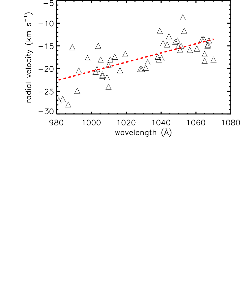
Figure 17: Example distribution of H₂ radial velocities for segment LiF2B, which had the largest correction to the slope of the wavelength solution (10 km s^-1 100 Å^-1). The dashed line shows the best linear fit. The slope was removed and a linear offset applied to match the radial velocity derived from our Keck observations of Na I (-5.1 km s^-1).

We made trial profile fits of H₂ lines with vpfit  to evaluate the accuracy of the relative wavelength scale within each segment. Radial velocity uncertainties for each H₂ line are $\sim 1$ km s^-1 (0.5 pixels). With $\sim 50$ H₂ lines per segment (save for the long wavelength ones LiF1B and LiF2A), linear dispersion corrections of 2–10 km s^-1 100 Å^-1 were applied, plus a zero point offset to make the H₂ velocities match the Na I heliocentric velocity of -5.1 km s^-1 measured from our Keck data. See Fig. 17 for an example. Standard deviations of radial velocity residuals after applying the linear corrections to each segment were 1–4 km s^-1 (0.5–2 pixels).

Appendix B Determination of the line spread function using H₂ lines

We made an independent determination of the FUSE instrumental profile (line spread function, LSF), which is poorly known. The LSF is suspected to vary with detector/channel/side segment, wavelength, time, pointing accuracy, and how accurately individual exposures are cross-correlated and summed (Kruk et al., 2002). The problem was also studied by Hébrard et al. (2002). Wood et al. (2002) attempted to solve for the LSF, coming up with a double Gaussian fit. We attempted to incorporate their solution into the FUSE LSF for profile fits with vpfit, but found that a single Gaussian gave better results based on the $\chi^{2}$ statistic. However, the FWHM of the Gaussian which gave the best fit varied between FUSE segments. We therefore decided to derive the FUSE LSF by using H₂ lines as fiducials. This was done by assuming the results from a combination of profile fitting with Owens (which leaves the LSF as a free parameter) and the COG method, and varying the width of a Gaussian LSF in km s^-1 for a each of a large number of H₂ lines. We only used unblended lines of the H₂ $J=2,3,4$ rotation levels, because the $J=0$ and 1 transitions are in the damping part of the curve of growth and are thereby mostly resolved, making them useless for assessing the LSF. (This is borne out by their showing uniformly inflated LSF FWHM values compared to the lower column density $J=2,3,4$ levels.) The number of H₂ lines fitted per segment was 29–45 except for the two long wavelength segments (LiF1B and LiF2A), which only had 4 and 7 respectively.

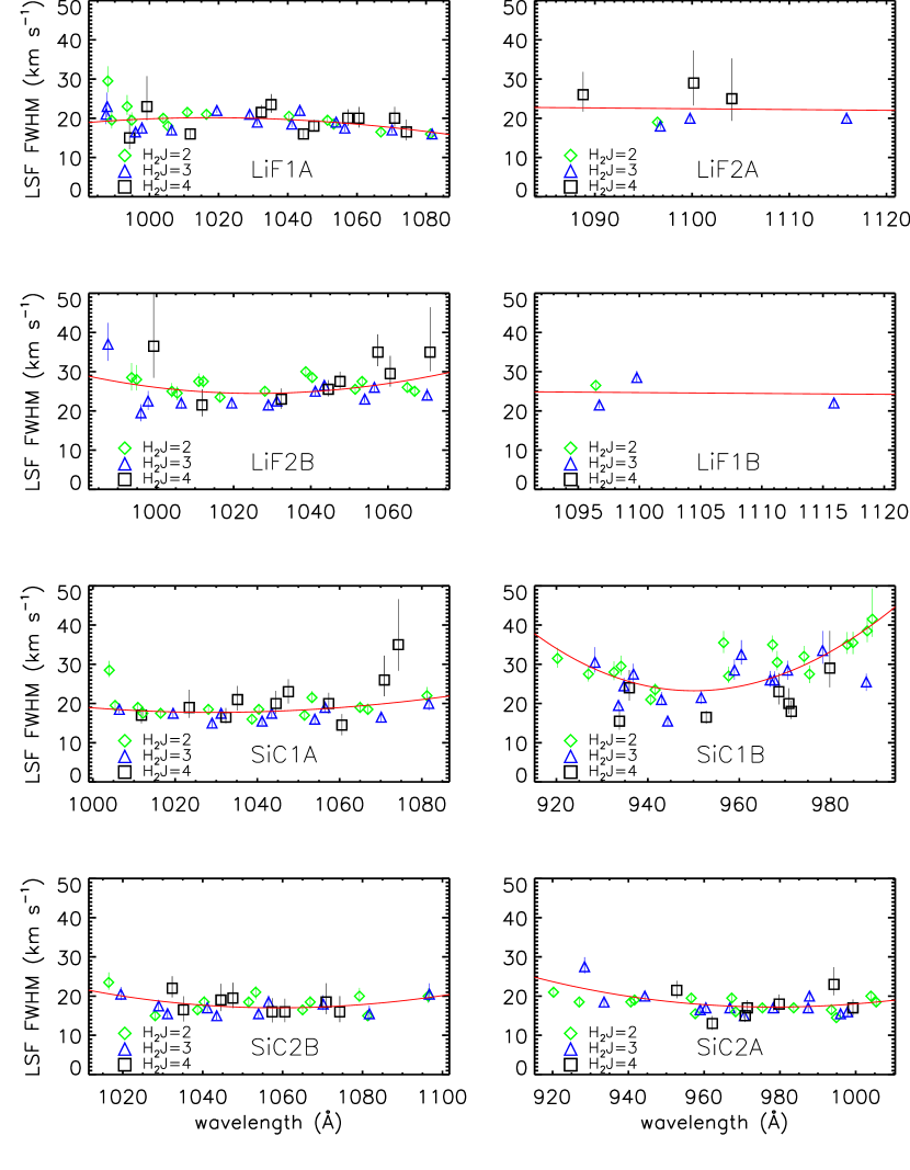
Figure 18: Fit to LSF for all segments, based on H₂ lines of rotation level $J=2,3,4$. Error bars are $1\sigma$.

vpfit can accommodate a line spread function which varies as a function of wavelength, and uses a power series in FWHM in Å as a function of wavelength. We therefore converted the FWHM from km s^-1 to Å and fitted a quadratic function to each of the segments using the interactive IRAF routine curfit, except in the case of LiF1B and LiF2A, which we fitted with simple constants in km s^-1. The root mean square of the LSF residuals ranged from 0.007–0.018 Å ($\sim 2.0-5.6$ km s^-1), with by far the worst fit for SiC1B. Plots for the LSF determinations are in Fig. 18.

Table 1: PG 0038$+$199 stellar properties

Quantity	Value	Reference
Galactic coordinates	$\ell=119.79^{\circ}$, $b=-42.66^{\circ}$	Green et al. (1986)
Spectral type	DO	Wesemael et al. (1993)
V	$14.544\pm 0.016$	Williams et al. (2001)
$T_{eff}$	115000$\pm 11500$ K	Dreizler & Werner (1996)
$\log g$	$7.5\pm 0.3$	Dreizler & Werner (1996)
Mass	0.59 M⊙	Dreizler & Werner (1996)
log(H/He)	$-0.7$	Dreizler et al. (1997)
log(N/He)	$-3$:	Dreizler & Werner (1996)
E(B-V)	${\lesssim}0.037$	Schlegel et al. (1998)
Distance	$297^{+164}_{-104}$ pc	this work

Table 2: H₂ and HD lines used for COG analysis.

			Equiv Width
Species	$\lambda$ (Å)	$\log f\lambda$	(mÅ)
H2 $J$=0	923.990	0.751	$125.0\pm 6.3$
H2 $J$=0	931.069	0.990	$137.7\pm 13.2$
H2 $J$=0	962.985	1.101	$200.6\pm 7.7$
H2 $J$=0	981.442	1.306	$265.0\pm 19.7$
H2 $J$=0	1077.141	1.100	$256.8\pm 8.2$
H2 $J$=0	1108.139	0.267	$116.5\pm 5.6$
H2 $J$=1	924.649	0.580	$106.5\pm 8.6$
H2 $J$=1	925.180	0.256	$98.9\pm 6.9$
H2 $J$=1	932.273	0.344	$117.3\pm 9.1$
H2 $J$=1	982.839	0.824	$222.0\pm 9.0$
H2 $J$=1	992.812	0.883	$277.8\pm 11.2$
H2 $J$=1	1003.300	0.929	$282.6\pm 9.3$
H2 $J$=1	1108.644	0.078	$155.9\pm 6.2$
H2 $J$=2	920.248	0.187	$38.0\pm 4.2$
H2 $J$=2	927.026	0.329	$54.9\pm 4.8$
H2 $J$=2	932.614	0.647	$61.2\pm 7.8$
H2 $J$=2	933.245	0.803	$82.6\pm 6.9$
H2 $J$=2	934.151	0.317	$45.1\pm 4.1$
H2 $J$=2	940.632	0.749	$51.1\pm 3.0$
H2 $J$=2	941.606	0.498	$53.7\pm 3.6$
H2 $J$=2	956.586	0.941	$63.4\pm 4.6$
H2 $J$=2	957.660	0.661	$58.2\pm 4.6$
H2 $J$=2	965.794	1.495	$83.4\pm 6.7$
H2 $J$=2	967.283	1.530	$90.9\pm 5.4$
H2 $J$=2	968.297	0.844	$68.9\pm 4.9$
H2 $J$=2	975.351	0.810	$62.3\pm 4.1$
H2 $J$=2	983.594	1.054	$70.3\pm 3.8$
H2 $J$=2	984.867	0.905	$64.4\pm 4.6$
H2 $J$=2	987.978	1.557	$99.1\pm 5.4$
H2 $J$=2	989.092	0.903	$48.2\pm 4.9$
H2 $J$=2	993.552	1.228	$96.6\pm 5.9$
H2 $J$=2	994.877	0.935	$92.3\pm 6.0$
H2 $J$=2	1003.988	1.222	$81.0\pm 4.4$
H2 $J$=2	1005.397	0.998	$64.1\pm 3.8$
H2 $J$=2	1009.030	1.200	$64.0\pm 4.3$
H2 $J$=2	1010.135	1.147	$57.2\pm 5.1$
H2 $J$=2	1010.945	1.381	$94.6\pm 4.0$
H2 $J$=2	1016.466	1.016	$75.8\pm 3.7$
H2 $J$=2	1038.695	1.234	$97.6\pm 5.2$
H2 $J$=2	1040.372	1.030	$79.5\pm 4.2$
H2 $J$=2	1051.505	1.168	$77.8\pm 4.0$
H2 $J$=2	1053.291	0.980	$74.9\pm 3.7$
H2 $J$=2	1065.001	1.057	$75.8\pm 4.7$
H2 $J$=2	1066.907	0.881	$85.3\pm 4.3$
H2 $J$=2	1079.227	0.868	$67.9\pm 5.5$
H2 $J$=2	1081.268	0.709	$79.4\pm 3.7$
H2 $J$=3	928.443	0.481	$32.4\pm 4.8$
H2 $J$=3	933.588	1.260	$41.4\pm 3.7$
H2 $J$=3	934.800	0.820	$51.2\pm 4.8$
H2 $J$=3	942.970	0.729	$47.2\pm 3.9$
H2 $J$=3	951.681	1.079	$49.1\pm 5.1$
H2 $J$=3	958.953	0.930	$50.0\pm 3.9$
H2 $J$=3	960.458	0.674	$46.0\pm 3.9$
H2 $J$=3	966.787	0.879	$39.5\pm 5.0$
H2 $J$=3	967.677	1.340	$58.1\pm 4.6$
H2 $J$=3	970.565	0.974	$53.4\pm 4.5$
H2 $J$=3	978.223	0.818	$46.2\pm 3.8$
H2 $J$=3	987.450	1.406	$48.8\pm 4.3$
H2 $J$=3	987.772	0.945	$51.7\pm 4.9$
H2 $J$=3	995.974	1.218	$65.0\pm 4.3$
H2 $J$=3	997.830	0.942	$59.4\pm 4.9$
H2 $J$=3	1006.417	1.199	$62.4\pm 4.1$
H2 $J$=3	1028.991	1.250	$55.2\pm 3.4$
H2 $J$=3	1031.198	1.059	$50.5\pm 3.2$
H2 $J$=3	1041.163	1.216	$68.6\pm 3.9$
H2 $J$=3	1043.508	1.052	$61.1\pm 3.5$
H2 $J$=3	1053.982	1.150	$54.8\pm 3.2$
H2 $J$=3	1056.479	1.006	$57.4\pm 3.2$
H2 $J$=3	1067.485	1.028	$54.1\pm 3.2$
H2 $J$=3	1070.148	0.909	$56.1\pm 3.6$
H2 $J$=3	1099.795	0.448	$46.6\pm 3.2$
H2 $J$=3	1115.907	-0.081	$36.9\pm 3.0$
H2 $J$=4	935.969	1.264	$29.5\pm 4.1$
H2 $J$=4	952.765	1.420	$33.7\pm 4.1$
H2 $J$=4	962.158	0.921	$19.4\pm 3.6$
H2 $J$=4	968.671	1.097	$26.9\pm 4.3$
H2 $J$=4	971.392	1.533	$33.1\pm 4.1$
H2 $J$=4	979.808	1.095	$22.8\pm 3.4$
H2 $J$=4	994.234	1.134	$21.3\pm 4.4$
H2 $J$=4	999.272	1.217	$23.5\pm 3.7$
H2 $J$=4	1011.818	1.154	$35.8\pm 3.0$
H2 $J$=4	1023.441	1.031	$22.2\pm 3.6$
H2 $J$=4	1032.355	1.247	$21.0\pm 3.0$
H2 $J$=4	1035.188	1.068	$27.3\pm 3.0$
H2 $J$=4	1044.548	1.206	$30.1\pm 3.2$
H2 $J$=4	1060.588	1.019	$20.4\pm 2.3$
HD $J$=0	959.817	1.150	$13.4\pm 4.0$
HD $J$=0	1007.283	1.515	$14.8\pm 3.2$
HD $J$=0	1011.457	1.423	$15.9\pm 2.7$
HD $J$=0	1042.848	1.332	$13.6\pm 2.2$
HD $J$=0	1054.288	1.238	$12.8\pm 2.3$
HD $J$=0	1066.271	1.089	10$6.6\pm 2.1$

Table 3: H₂ and HD Column Densities.

000Species000	000000$J$000000	000Adopted ($2\sigma$)  000
H2	0	$18.76\pm 0.05$
H2	1	$19.18\pm 0.05$
H2	2	$17.73\pm 0.40$
H2	3	$16.74\pm 0.40$
H2	4	$14.63\pm 0.15$
H2	5	$14.04\pm 0.15$
H2	total	$19.33\pm 0.04$
HD	0	$13.95\pm 0.10$

Table 4: Atomic lines used for column density measurements

Species	$\lambda$ (Å)	$\log f\lambda$
H I	919.351	0.043
H I	920.963	0.168
H I	923.150	0.312
H I	926.226	0.471
H I	1025.722	1.909
D I	919.102	0.043
D I	920.712	0.170
D I	922.899	0.311
D I	925.974	0.470
D I	1025.443	1.909
C I	945.191	2.157
C I	1111.421	0.996
C I	1122.438	0.820
C I	1129.193	0.998
C I	1139.793	1.206
C I	1157.910	1.451
C I	1158.324	0.810
C I∗	945.338	2.157
C II	1036.337	2.102
C III	977.020	2.875
N I	951.079	-0.794
N I	952.523	-0.401
N II	1083.994	2.072
O I	974.070	-1.807
Na I	5891.583	3.596
Na I	5897.558	3.296
Si II	1020.699	1.188
P II	1152.818	2.435
S III	1012.501	1.634
Ar I	1048.220	2.408
Fe II	940.192	1.056
Fe II	1055.262	0.926
Fe II	1081.875	1.180
Fe II	1096.877	1.545
Fe II	1121.975	1.351
Fe II	1125.448	1.093
Fe II	1127.098	0.529
Fe II	1133.665	0.833
Fe II	1142.366	0.757
Fe II	1143.226	1.182

Table 5: Atomic Column Densities.

Ion	Adopted	Errors		Technique
	Value	$1\sigma$	$2\sigma$
H I	$\geq$o$20.41$	0.04	0.08	PF (3)
H I+2H2	$\geq$o$20.48$	0.04	0.07	PF, COG
D I	$\geq$o$15.75$	0.04	0.08	PF (3)
D I+HD	$\geq$o$15.76$	0.04	0.08	PF, COG
C I	$\geq$o$13.80$	0.04	0.08	PF (2)
C I∗	$\geq$o$13.25$	0.19	${}^{+0.32}_{-0.54}$	PF (1)
C II	$\geq$ 14.47	$\cdots$	$\cdots$	AOD
C III	$\geq$ 13.95	$\cdots$	$\cdots$	AOD
N I	$\geq$o$16.39$	${}^{+0.07}_{-0.10}$	${}^{+0.14}_{-0.18}$	PF (3)
N II	$\geq$ 14.12	$\cdots$	$\cdots$	AOD
O I	$\geq$o$17.37$	${}^{+0.08}_{-0.15}$	${}^{+0.15}_{-0.25}$	PF (3)
Na I	$\geq$o$12.19$	0.03	0.04	AOD, PF (2)
Si II	$\geq$ 15.17	$\cdots$	$\cdots$	AOD
P II	$\geq$ 13.34	$\cdots$	$\cdots$	AOD
S III	$\geq$o$13.98$	${}^{+0.03}_{-0.06}$	${}^{+0.07}_{-0.10}$	PF (1)
Ar I	$\geq$ 13.35	$\cdots$	$\cdots$	AOD
Fe II	$\geq$o$14.42$	${}^{+0.03}_{-0.02}$	${}^{+0.06}_{-0.05}$	PF (3),COG

Table 6: Unidentified lines in FUSE data for PG 0038$+$199 

Wavelength range (Å)	Wavelength range (Å)	Wavelength range (Å)
973.0 - 973.2	1062.2 - 1062.4	1144.7 - 1144.9
976.6 - 976.8	1067.0 - 1067.2	1146.0 - 1146.5
997.3 - 997.5	1071.9 - 1072.1	1146.55 - 1146.8
999.5 - 999.8	1073.65 - 1073.85	1147.2 - 1147.4
1014.6 - 1014.8	1080.35 - 1080.7	1147.9 - 1148.1
1051.9 - 1052.1	1080.95 - 1081.10	1173.45 - 1173.89
1052.6 -1052.8	1125.15 - 1125.35	1180.48 - 1180.68
1061.3 - 1061.5	1141.1 - 1141.3

Table 7: D I, H I, O I, N I, HD, H₂ ratios.

Species	Ratio	Errors ($1\sigma$)	Errors ($2\sigma$)
$10^{5}$[D I + HD]/[H I + 2H2]	$1.91$	$+0.26\,-0.24$	$+0.52\,-0.42$
$10^{5}$D/H	$2.19$	$+0.30\,-0.27$	$+0.55\,-0.50$
$10^{4}$O/[H+2H2]	$7.76$	$+1.78\,-2.33$	$+3.38\,-3.49$
$10^{4}$O/H	$8.51$	$+1.99\,-2.56$	$+4.09\,-3.86$
$10^{4}$N/[H+2H2]	$0.81$	$+0.17\,-0.18$	$+0.36\,-0.29$
$10^{4}$N/H	$0.95$	$+0.20\,-0.20$	$+0.43\,-0.34$
$10^{2}$[D I + HD]/O I	$2.63$	$+1.13\,-0.49$	$+2.18\,-0.85$
$10^{2}$D/O	$2.40$	$+1.03\,-0.45$	$+2.19\,-0.78$
$10^{1}$[D I + HD]/N I	$2.34$	$+0.66\,-0.39$	$+1.35\,-0.72$
$10^{1}$D/N	$2.29$	$+0.65\,-0.39$	$+1.32\,-0.71$
$10^{2}$N/O	$1.12$	$+0.52\,-0.28$	$+1.05\,-0.47$
$10^{6}$HD/H2	$4.17$	$\cdots$	$+0.68\,-0.49$

Figure 1: FUSE data for PG 0038$+$199 with ISM and geo-coronal ($\oplus$) identifications. Data are binned by four pixels, scaled and merged for presentation only. Photospheric lines of Si IV are marked with dashed lines. We could not identify some absorption lines, particularly in the range 1080–1180 Å (Table 6; a stellar origin is suspected).

Figure 3: Top panel: Apparent column density per velocity unit for the Na I doublet observed toward PG 0038$+$199. The $f$-values of the two transitions differ by a factor of 2. A small amount of unresolved saturation can be seen in the range $-12<v<-1$ km s^-1  where the profile of the stronger line falls below that of the weaker line. Bottom two panels: Owens fit to the Keck HIRES data.

Figure 4: Single-component COG for H₂ and HD along the PG 0038$+$199 sight line. A different symbol is used for each $J$ level. The $J=5$ level was not included because the equivalent widths for its transitions are too small.

Figure 5: Excitation for H₂ along the PG 0038$+$199  line of sight, using the adopted values from Table 3. H₂ J levels are marked at top. See text for details.

Figure 6: Owens profile fit to O I  showing the fit before convolution with the local LSF (light blue line) and after convolution (red line). Flux is in erg cm^-2 s^-1 Å^-1. See stand-alone JPEG file.

Figure 10: The H I 21 cm flux in units of brightness temperature vs. radial velocity toward PG 0038$+$199 from the Leiden-Dwingeloo survey.

Figure 11: Ratios, with $1\sigma$ and $2\sigma$ errors, for [D I+HD], [H I+2H₂], O I, N I column densities. Best fit values are shown by asterisks.

Figure 12: (a) D/H and $1\sigma$ error bars plotted vs. line-of-sight distance, using D/H measurements in Wood et al. (2004) and this work (red). Different symbols are used for different sources of the D I measurement. Red open boxes: PG 0038$+$199, representing D/H (upper box) and [D I + HD]/[H I + 2H₂] (lower box), slightly offset in distance for clarity. (b) D/H plotted vs. line-of-sight H I column density. The symbols are the same as in (a), specifically that the red open boxes represent PG 0038$+$199, showing the H I column density (upper box) and the [H I+ 2H₂] column density (lower box). Black horizontal and dotted lines: weighted means and $1\sigma$ standard deviations as a function of $N(\mbox{{H~{}I}})$ from Wood et al. Red solid and dashed lines: the primordial D/H value (Kirkman et al., 2003; O’Meara et al., 2001; Pettini & Bowen, 2001; Levshakov et al., 2002) and lower $1\sigma$ standard deviation, respectively. For intermediate values $19.2<\log N(\mbox{{H~{}I}})<20.5$, D/H appears variable.

References

- Abgrall et al. (1993a) Abgrall, H., Roueff, E., Launay, F., Roncin, J.-Y., Subtil, J.-L. 1993, A&AS, 101, 273
- Abgrall et al. (1993b) Abgrall, H., Roueff, E., Launay, F., Roncin, J.-Y., Subtil, J.-L. 1993, A&AS, 101, 323
- André et al. (2003) André, M. K. et al. 2003, ApJ, 591, 1000
- Biémont & Zeippen (1992) Biémont, E., & Zeippen, C. S. 1992, A&A, 265, 850
- Black & Dalgarno (1973) Black, J. H. & Dalgarno, A. 1973, ApJ, 184, L101
- Burles (2000) Burles, S. 2000, Nucl. Phys. A, 663, 861
- Burles et al. (2001) Burles, S., Nollett, K. M., & Turner, M. S. 2001, ApJ, 552, L1
- Carswell et al. (1996) Carswell, R. F., Webb, J. K., Lanzetta, K. M., Baldwin, J. A., Cooke, A. J., Williger, G. M., Rauch, M., Irwin, M. J., Robertson, J. G., Shaver, P. A. 1996, MNRAS, 278, 506
- Cartledge et al. (2004) Cartledge, S. I. B., Lauroesch, J. T., Meyer, D. M., Sofia, U. J. 2004, ApJ, in press
- Cha et al. (2000) Cha, A. N. S., Sahu, M. S., Moos, H. W., Blaauw, A. 2000, ApJS, 129, 281
- Chiappini, Renda, & Matteucci (2002) Chiappini, C., Renda, A., & Matteucci, F. 2002, A&A, 395, 789
- Crighton et al. (2003) Crighton, N. H. M., Webb, J. K., Carswell, R. F., Lanzetta, K. M. 2003, MNRAS, 345, 243
- Cyburt et al. (2003) Cyburt, R., H., Fields, B. D., & Olive, K. A. 2003, Physics Letters B, 567, 227
- deAvillez & MacLow (2002) deAvillez, M. A., & MacLow, M.-M. 2002, ApJ, 581, 1047
- Draine (2004) Draine, B. T. 2004, to appear in “Carnegie Observatories Astrophysics Series, Vol. 4: Origin and Distribution of the Elements”, ed. A. McWilliam and M. Rauch (Cambridge: Cambridge Univ. Press), astro-ph/0312592
- Dreizler et al. (1997) Dreizler, S., Werner, K., Heber, U., Reid, N., Hagen, H. 1997, in The Third Conference on Faint Blue Stars, ed. A. G. D. Philip, J. Liebert, R. Saffer, D. S. Hayes (L. Davis Press), 303
- Dreizler & Werner (1996) Dreizler, S., & Werner, K. 1996, A&A, 314, 217
- Ferlet et al. (2000) Ferlet, R. et al. 2000, ApJ, 538, 69
- Ferlet, Vidal-Madjar & Gry (1985) Ferlet, R., Vidal-Madjar, A., & Gry, C. 1985, ApJ, 298, 838
- Fitzpatrick & Spitzer (1994) Fitzpatrick, E. L. & Spitzer, L., Jr. 1994, ApJ, 427, 232
- Friedman et al. (2002) Friedman, S. D., et al. 2002, ApJS, 140, 37
- Green et al. (1986) Green, R. F., Schmidt, M., & Liebert J. 1986, ApJS, 61, 305
- Haffner et al. (2003) Haffner, L. M., Reynolds, R. J., Tufte, S. L., Madsen, G. J., Jaehnig, K. P., Percival, J. W. 2003, ApJS, 149, 405
- Hartmann & Burton (1997) Hartmann, L. & Burton, W. B. 1997, Atlas of Galactic Neutral Hydrogen. Cambridge Univ. Press, ISBN 0521471117
- Hébrard et al. (2002) Hébrard, G. et al., ApJS, 140, 103
- Hébrard & Moos (2003) Hébrard, G. & Moos, H. W. 2003, ApJ, 599, 297
- Hébrard et al. (2004) Hébrard, G., Chayer, P., Dupuis, J., Moos, H. W., Sonnentrucker, P., Tripp, T. M., Williger, G. M. 2004, Astrophysics in the Far UV: Five Years of Discovery with FUSE, ed. Sonneborn, G., Moos, H. W. & Andersson, B.-G., ASP Conf. Series, in prep.
- Hoopes et al. (2003) Hoopes, C. G., Sembach, K. R., Hébrard, G., Moos, H. W., & Knauth, D. C. 2003, ApJ, 586, 1094
- Howk et al. (2000) Howk, J. C., Sembach, K. R., Roth, K. C., Kruk, J. W. 2000, ApJ, 544, 867
- Hubeny & Lanz (1995) Hubeny, I., & Lanz, T. 1995, ApJ, 439, 875
- Jenkins (1986) Jenkins, E. B. 1986, ApJ, 304, 739
- Jenkins, Savage, & Spitzer (1986) Jenkins, E.B., Savage, B.D., & Spitzer, L., Jr. 1986, ApJ, 301, 355
- Jenkins et al. (1999) Jenkins, E. B., Tripp, T. M., Wożniak, P. R., Sofia, U. J., & Sonneborn, G. 1999, ApJ, 520, 182
- Jenkins et al. (2000) Jenkins, E. B., Wożniak, P. R., Sofia, U. J., Sonneborn, G., Tripp, T. M. 2000, ApJ, 538, 275
- Kirkman et al. (2003) Kirkman, D., Tytler, D., Suzuki, N., O’Meara, J. M., & Lubin, D. 2003, ApJS, 149, 1
- Kohoutek (1997) Kohoutek, L. 1997, Astron. Nachr., 318, 35
- Kruk et al. (2002) Kruk, J. W., et al. 2002, ApJS, 140, 19
- Lacour et al. (2004) Lacour, S., André, M. K., Sonnentrucker, P., LePetit, F., Welty, D. E., Desert, J.-M., Ferlet, R., Roueff, E., York, D. G. 2005, A&A, 430, 967
- Laurent et al. (1979) Laurent, C., Vidal-Madjar, A., & York, D. G. 1979, ApJ, 229, 923
- Lemoine et al. (1999) Lemoine, M. et al. 1999, NewA, 4, 231
- Lemoine et al. (2002) Lemoine, M. et al. 2002, ApJS, 140, 67
- Levshakov et al. (2002) Levshakov, S. A., Dessanges-Zavadsky, M., D’Odorico, S., & Molaro, P. 2002, ApJ, 565, 696
- Linsky (1998) Linsky, J. L. 1998, Space Sci. Rev., 84, 285
- Lipshtat et al. (2004) Lipshtat, A., Ofer, B., & Herbst, E. 2004, MNRAS, 348, 1055
- Liszt (2003) Liszt, H. 2003, A&A, 398, 621
- Messenger (2000) Messenger, S. 2000, Nature, 404, 968
- Meyer, Cardelli, & Sofia (1997) Meyer, D. M., Cardelli, J. A., & Sofia, U. J. 1997, ApJ, 490, L103
- Meyer, Jura, & Cardelli (1998) Meyer, D. M., Jura, M., & Cardelli, J. A. 1998, ApJ, 493, 222
- Morton (1991) Morton, D. C., 1991, ApJS, 77, 119
- Morton (2003) Morton, D. C., 2003, ApJS, 149, 205
- Moos et al. (2000) Moos, H. W. et al. 2002, ApJ, 538, L1
- Moos et al. (2002) Moos, H. W. et al. 2002, ApJS, 140, 3
- Oliveira et al. (2003) Oliveira, C. M., Hébrard, G., Howk, J. K., Kruk, J. W., Chayer, P., & Moos, H. W. 2003, ApJ, 587, 235
- O’Meara et al. (2001) O’Meara, J. M., Tytler, D., Kirkman, D., Suzuki, N., Prochaska, J. X., Lubin, D., & Wolfe, A. M. 2001, ApJ, 552, 718
- Peeters et al. (2004) Peeters, E., Allamandola, L. J., Bauschlicher, C. W., Jr., Hudgins, D. M., Sandford, S. A., Tielens, A. G. G. M. 2004, ApJ, 604, 252
- Pettini & Bowen (2001) Pettini, M., & Bowen, D. V. 2001, ApJ, 560, 41
- Rachford et al. (2002) Rachford, B. L. et al. 2002, ApJ, 577, 221
- Rachford et al. (2001) Rachford, B. L. et al. 2001, ApJ, 555, 839
- Rauch, Kerber, & Pauli (2004) Rauch, T., Kerber, F., & Pauli, E.-M. 2004, A&A, 417, 647
- Romano et al. (2003) Romano, D., Tosi, M., Matteucci, F., & Chiappini, C. 2003, MNRAS, 346, 295
- Sahnow et al. (2000) Sahnow, D. J., et al. 2000, ApJ, 538, L7
- Savage et al. (1977) Savage, B. D., Drake, J. F., Budich, W., & Bohlin, R. C. 1977, ApJ, 216, 291
- Savage & Mathis (1979) Savage, B. D. & Mathis, J. S. 1979, ARAA, 17, 73
- Savage & Sembach (1991) Savage, B. D., & Sembach, K. R. 1991, ApJ, 379, 245
- Schlegel et al. (1998) Schlegel, D. J., Findbeiner, D. P., & Davis, M. 1998, ApJ, 500, 525
- Schramm & Turner (1998) Schramm, D. N., & Turner, M. S. 1998, Rev. Mod. Phys., 70, 303
- Sembach & Savage (1992) Sembach, K. R., & Savage, B. D. 1992, ApJS, 83, 147
- Sembach et al. (2004) Sembach, K. R., et al. 2004, ApJS, 150, 387
- Sfeir et al. (1999) Sfeir, D. M., Lallement, R., Crifo, F., & Welsh, B. Y. 1999, A&A, 346, 785
- Snow et al. (2000) Snow, T. P. et al. 2000, ApJ, 538, 65
- Snowden et al. (1995) Snowden, S. L. et al. 1995, ApJ, 454, 643
- Sonneborn et al. (2000) Sonneborn, G., Tripp, T. M., Ferlet, R., Jenkins, E. B., Sofia, U. J., Vidal-Madjar, A., Wozniak, P. R. 2000, ApJ, 545, 277
- Spitzer (1985) Spitzer, L., Jr. 1985, ApJ, 290, L21
- Spitzer, Cochran, & Hirschfeld (1974) Spitzer, L., Jr., Cochran, W. D., & Hirschfeld, A. 1974, ApSS, 28, 373
- Steigman (2003) Steigman, G. 2003, ApJ, 586, 1120
- Stephenson & Green (2002) Stephenson, F. R. & Green, D. A. 2002, “Historical Supernovae and their Remnants” (Oxford: Clarendon Press), ISBN 0198507666
- Verner, Barthel, & Tytler (1994) Verner, D. A., Barthel, P. D., & Tytler, D. 1994, A&AS, 108, 287
- Vogt et al. (1994) Vogt, S. S., et al. 1994, Proc. SPIE, 2198, 362
- Webb (1987) Webb, J. K. 1987, PhD thesis, Cambridge University
- Webb (1991) Webb, J. K., Carswell, R. F., Irwin, M. J., Penston, M. V. 1991, MNRAS, 250, 657
- Welty et al. (1999) Welty, D. E., Hobbs, L. M., Lauroesch, J. T., Morton, D. C., Spitzer, L., Jr., York, D. G. 1999, ApJS, 124, 465
- Werner et al. (1997) Werner, K., Bagschik, K., Rauch, T., Napiwotzki, R. 1997, A&A, 327, 721
- Wesemael et al. (1993) Wesemael, F., Greenstein, J. L., Liebert, J., Lamontagne, R., Fontaine, G., Bergeron, P., & Glaspey, J. W. 1993, PASP, 105, 761
- Wiese, Fuhr & Deters (1996) Wiese, W. L., Fuhr, J. R., & Deters, T. M. 1996, J. Phys. Chem. Ref. Data Monogr. 7
- Williams et al. (2001) Williams, T., McGraw, J.T., Mason, P.A., & Grashius, R. 2001, PASP, 113, 490
- Wood et al. (2002) Wood, B. E., Linsky, J. L., Hébrard, G., Vidal-Madjar, A., Lemoine, M., Moos, H. W., Sembach, K. R., & Jenkins, E. B. 2002, ApJS, 140, 91
- Wood et al. (2004) Wood, B. E., Linsky, J. L., Hébrard, G., Williger, G. M., Moos, H. W., & Blair, W. P. 2004, ApJ, 609, 838
- York & Rogerson (1976) York, D. G., & Rogerson, J. B. 1976, ApJ, 203, 378
- York (1983) York, D. G. 1983, ApJ, 264, 172
- Zuckerman & Reid (1998) Zuckerman, B. & Reid, I. N. 1998, ApJ, 505, L143