X-ray variability, viscous time scale and Lindblad resonances in LMXBs.

Abstract

Based on RXTE/ASM and EXOSAT/ME data we studied X-ray variability of persistent LMXBs in the $\sim 10^{-8}-10^{-1}$ Hz frequency range, aiming to detect features in their power density spectra (PDS) associated with the viscous time scale of the accretion disk $t_{\rm visc}$. As this is the longest intrinsic time scale of the disk, the power density of its $\dot{M}$ variations is expected to be independent on the frequency at $f\la 1/t_{\rm visc}$. Indeed, in the PDS of 11 sources out of 12 we found very low frequency break, below which the spectra are nearly flat. At higher frequencies they approximately follow the $P_{\nu}\propto\nu^{-1.3}$ law.

The break frequency correlates very well with the binary orbital frequency in a broad range of binary periods $P_{\rm orb}\sim 12{\rm~{}min}-33.5{\rm~{}days}$, in accord with theoretical expectations for the viscous time scale of the disk. However, the value of $f_{\rm break}/f_{\rm orb}$ is at least by an order of magnitude larger than predicted by the standard disk theory. This suggests that a significant fraction of the accretion $\dot{M}$ occurs through the optically thin and hot coronal flow with the aspect ratio of $H/R\ga 0.1$. The predicted parameters of this flow, $T\sim 10^{4}-10^{6}$ K and $n_{e}\sim 10^{12}-10^{15}$ cm^-3 are in qualitative agreement with recent Chandra and XMM-Newton observations of complex absorption/emission features in the spectra of LMXBs with high inclination angle.

We find a clear dichotomy in the value of $t_{\rm visc}/P_{\rm orb}$ between wide and compact systems, the compact systems having $\sim 10$ times shorter viscous time. The boundary lies at the mass ration $q\approx 0.3$, suggesting that this dichotomy is caused by the excitation of the 3:1 inner Lindblad resonance in low-$q$ LMXBs.

1 Introduction

X-ray binaries show X-ray flux variations in a broad range of time scales (Fig.1). Their power density spectra often reveal a number of periodic and quasi-periodic phenomena, corresponding to the orbital frequency of the binary system, the spin frequency of the neutron star and quasi-periodic oscillation, which nature is still poorly understood. In addition, aperiodic variability is observed, giving rise to the broad band continuum component in power density spectra, extending from $\sim 10-100$ msec to the longest time scales accessible for monitoring instruments.

The aperiodic variability is often characterized by the fractional rms values of $\sim$ tens of per cent, indicating that variations of the mass accretion rate $\dot{M}$ in the broad range of time scales are present in the innermost region of the accretion flow, where X-ray emission is produced. From the point of view of characteristic time scales, the high frequency variations could potentially be produced in the vicinity of the compact object. Longer time scales, on the contrary, exceed by many orders of magnitude the characteristic time scales in the region of the main energy release. Hence, the low frequency $\dot{M}$ variations have to be generated in the outer parts of the accretion flow and to be propagated to the region of the main energy release. Due to the diffusive nature of the standard Shakura-Sunyaev disk (Shakura & Sunyaev, 1973), it plays the role of the low-pass filter, at any given radius $r$ suppressing $\dot{M}$ variations on the time scales shorter than the local viscous time $t_{\rm visc}(r)$. The viscous time is, on the other hand, the longest time scale of the accretion flow. Hence, it is plausible to suppose that any given radius $r$ contributes to $\dot{M}$ and X-ray flux variations predominantly at the frequency $f\sim 1/t_{\rm visc}(r)$ (Lyubarskii, 1997; Churazov et al., 2001). Lyubarskii (1997) demonstrated that in this picture $P_{\nu}\propto\nu^{-\alpha}$ power density spectra can naturally appear with slope $\alpha\sim 1$, in good agreement with observations.

Owing to the finite size of the accretion disk, the longest time scale which can appear in the disk is restricted by the viscous time on its outer boundary $t_{\rm visc}(R_{d})$. Below this frequency the X-ray flux variations are uncorrelated, therefore the power density spectrum of the accretion disk should become flat at $f\la f_{\rm visc}\sim 1/t_{\rm visc}(R_{d})$. If there are several components in the accretion flow each having a different viscous time scale (e.g. geometrically thin disk and diffuse corona above it), several breaks can appear on the power spectra at the frequencies, corresponding to the inverse viscous time scale of each component. Yet another source of $\dot{M}$ variations might be the variability of the mass transfer rate from the donor star. As these variations also have to be propagated through the accretion disk, only low frequency perturbations, with $f\la 1/t_{\rm visc}(R_{d})$, will reach the region of the main energy release. This might give rise to an independent continuum component in the power density spectrum at $f\la 1/t_{\rm visc}(R_{d})$. The shape of the final power density spectrum of X-ray binary will depend on the relative amplitudes of the $\dot{M}$ variations due to different components of the accretion flow and the donor star. As these are independent from each other, a distinct features should appear in the power density spectrum of X-ray binary at frequencies $f\sim 1/t_{\rm visc}(R_{d})$.

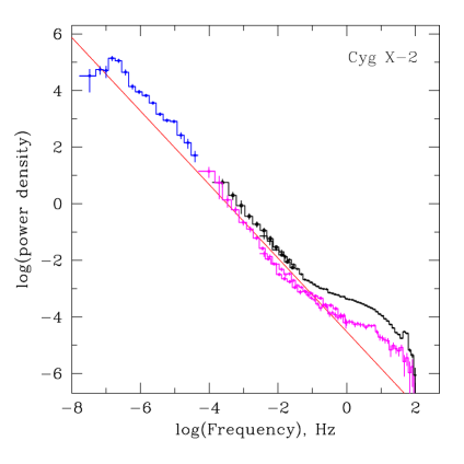
Figure 1: The power spectrum of Cyg X-2 in broad frequency range. Based on non-simultaneous ASM, PCA and EXOSAT data. The solid line shows $P_{\nu}=1\cdot 10^{-4}\,\nu^{-1.3}$ power law.

The viscous time scale of the accretion disk is (Shakura & Sunyaev, 1973)

$$t_{\rm visc}=\frac{2}{3\alpha}\,\left(\frac{H_{d}}{R_{d}}\right)^{-2}\frac{1}{\Omega_{K}(R_{d})}$$ (1)

where $H_{d}$ is the disk half thickness and $\Omega_{K}(R_{d})$ is the Keplerian frequency at the outer disk boundary $R_{d}$. For a geometrically thin disk, $H/R\ll 1$, the viscous time scale is significantly longer than the Keplerian time at the outer disk boundary. If the disk fills a large fraction of the Roche-lobe of the primary, as is the case for steady disks in persistent LMXBs, $R_{d}\sim 0.7-0.9\,R_{L}$, (section 4.3), the viscous time at the outer boundary $t_{\rm visc}(R_{d})$ will exceed the orbital period of the binary system $P_{orb}$ as well. Therefore, one might expect to find features associated with the viscous time of the accretion disk at frequencies below the orbital frequency of the binary system. Detection of such features for a sample of LMXBs would give an opportunity to probe the accretion disk parameters, such as viscosity parameter $\alpha$ and the disk thickness at its outer boundary.

In this paper we study a sample of persistent low mass X-ray binaries aiming to detect such features in their power density spectra. Longevity of typical orbital periods in LMXBs requires long monitoring observations to achieve this goal. This has become possible thanks to the long operations of the All Sky Monitor aboard Rossi X-ray Timing Explorer, which provided long term light curves of hundreds of galactic sources covering period of $\sim 7-8$ years. Some sources with rather short orbital period, $\la$ few hours may be studied based on the EXOSAT data.

Table 1: The binary system parameters for LMXBs from the ASM and EXOSAT samples.

Source	$M_{1}$	$M_{2}$	$P_{\rm orb}$	$a$	q	$i$	D	Ref.
	$M_{\odot}$	$M_{\odot}$	hrs	$10^{10}$ cm		$\deg$	kpc
	(1)	(2)	(3)	(4)	(5)	(6)	(7)	(8)
ASM sample
GRS 1915+105	$14.0\pm 4.4$	$0.81\pm 0.53$	$804\pm 36$	$747\pm 78$	$0.058\pm 0.033$	$66\degr\pm 2\degr$	$12.1\pm 0.8$	1,2
GX 13+1	1.4	$5\pm 1$ a	592.8	$461\pm 25$	$3.6\pm 0.9$	—	$7\pm 1$	3
Cir X-1	1.4	$4\pm 1$	398.4	$334\pm 21$	$2.9\pm 0.8$	—	$5.5$	4
Cyg X-2	$1.78\pm 0.23$	$0.60\pm 0.13$	236.3	$180\pm 7$	$0.34\pm 0.04$	$62.5\pm 4\degr$	$7.2\pm 1.1$	5
GX 349+2	1.4	$1.5\pm 1$	22.5$\pm$0.1	$40.0\pm 4.7$	$1.07\pm 0.73$	—	$9.2$	6
Sco X-1	1.4	0.42	18.92	$30.5\pm 1.1$	$0.30\pm 0.05$	$38\degr$	$2.8\pm 0.3$	7
EXOSAT sample
EXO 0748-676	1.4	$0.45$	$3.824$	$10.6\pm 0.4$	$0.32\pm 0.06$	$\sim 75\degr$	$7.6$	8
4U 1636-536	$1.4$	$0.36$	$3.793$	$10.3\pm 0.4$	$0.26\pm 0.05$	—	5.9	9
4U 1323-619	1.4	0.26	2.93	$8.53\pm 0.35$	$0.19\pm 0.03$	$\la 80\degr$	$15\pm 5$	9
4U 1916-053	1.4	$0.09\pm 0.02$	0.83	$3.55\pm 0.16$	$0.064\pm 0.017$	$\ga 70\degr$	10.0	10
1H 1627-673	$1.4$	$0.08\pm 0.01$	$0.690$	$3.13\pm 0.14$	$0.057\pm 0.011$	$\la 8\degr$	8.0 11,12
4U 1820-303	$1.4$	$0.07\pm 0.01$	$0.190$	$1.32\pm 0.06$	$0.050\pm 0.010$	—	8.0	13

(1) – the mass of the compact object, if the uncertainty is not given $\sigma=0.2M_{\odot}$ is assumed; (2) – the mass of the secondary, if the uncertainty is not given, $10\%$ relative error is assumed; (3) – orbital period; (4) – binary separation computed from the 3rd Kepler law; (5) – mass ratio $q=M_{1}/M_{2}$. For GRS 1915+105 and Cyg X-2 from refs (1) and (5) respectively, for other sources computed from the masses given in the columns (1) and (2) of the table. (6) – inclination; (7) – source distance; (8) – reference for binary system parameters: ¹ Harlaftis & Greiner 2004; ² Fender et al. 1999; ³ Bandyopadhyay et al. 1999; ⁴ Johnston et al. 1999; ⁵ Orosz and Kuulkers 1999; ⁶ Wachter & Margon 1996; ⁷ Steeghs and Casares 2002; ⁸ Parmar et al. 1986; ⁹ an estimate based on the empirical $P_{orb}-$mass relation from Patterson, 1984; ¹⁰ Nelson et al. 1986; ¹¹ Levine et al. 1988; ¹² Chakrabarty 1998; ¹³ Rappaport et al. 1987; ^a the companion mass estimate is very uncertain.

The paper is structured as follows. In section 2 we describe the selection criteria and sample of LMXBs. Power density spectra and their approximations are presented in the section 3. The viscous time scale of the accretion disks as obtained from the power spectra analysis and constrains on parameters of the outer disk are discussed in the section 4. In section 5 we consider the vertical structure of the semi-thick accretion flow, derive parameters of the disk corona and compare these with other evidence of the existence of diffuse coronal flow in LMXBs. Our results are summarized in section 6. In the Appendix we describe the method used to calculate power density spectra from the ASM light curves.

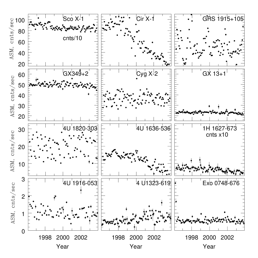
Figure 2: Long term X-ray light curves of selected sources obtained by ASM (2–12 keV). The light curves cover the period from 1996–2004

2 The data and selection criteria

2.1 Data

We used data of the ASM instrument of RXTE observatory (Swank, 1999), covering the period from 1996–2004 (MJD range from $\approx 50100-53100$). The ASM instrument operates in the 2–12 keV energy range and performs flux measurements for over $\sim 300$ X-ray sources from the ASM source catalog once per satellite orbit, i.e. every $\sim 90$ min. Each flux measurement (dwell) has duration of $\sim 90$ sec. Due to navigational constrains and appearance of very bright transient sources, the ASM light curves for individual sources sometimes have gaps of duration of up to few months. The dwell-by-dwell light curves were retrieved from the public RXTE/ASM archive at HEASARC.

For sources with short orbital periods, $P_{\rm orb}\la 4$ hours, we used the data of the medium energy (ME) detector of EXOSAT satellite (Turner, Smith & Zimmermann, 1981). It provided $\sim$ several tens of ksec long light curves with typical time resolution of $\sim 1$ sec in the 0.9–8.9 keV energy range. The EXOSAT data were also retrieved from HEASARC.

2.2 Selection criteria

We have selected low mass X-ray binaries, satisfying the following criteria:

1. Persistent sources, which light curves do not show off-states or X-ray Novae-like outbursts. This ensures that the accretion disk was in the same state during the analyzed period.

2. The orbital period $P_{orb}$ is known. Orbital parameters of X-ray sources were taken from the catalog of Liu et al. (2001).

   The Nyquist frequency in the power density spectra obtained from the ASM light curves, $f_{\rm Nyq}\sim 10^{-4}$ Hz, correspond to period of $\sim 3$ hours. In practice, due to specifics of the ASM light curves, the high frequency part of the power spectra can sometimes be distorted by the aliasing effect. To minimize the contribution of this effect we selected source with sufficiently long orbital periods, $P_{\rm orb}\ga 10$ hours.

   Although the aliasing is not an issue for EXOSAT light curves, their duration, typically limited by $\sim 50$ ksec, imposes a different constrains on the $P_{\rm orb}$. As we are looking for features at the time scales larger than $P_{\rm orb}$, we required that the light curve covers at least several $P_{\rm orb}$. This leads to the constrain for the sources which can be studied using EXOSAT light curves, $P_{orb}\la 4$ hours.

3. Source brightness. We selected sources with the average count rate exceeding $\ga 2$ cnts/s for ASM and $\ga 5$ cnts/s for EXOSAT.

4. The noise level, calculated for ASM power spectra, although approximately correct, is not accurate enough, due to existence of unaccounted systematic errors in the flux measurements (e.g. Grimm et al., 2002). To avoid additional uncertainties in the power spectra we considered only sources with sufficiently high signal at the orbital frequency, $P_{\rm signal}\ga 10P_{\rm noise}$ at $f_{\rm orb}$. For EXOSAT light curves the noise level is not an issue.

2.3 The sample

There are 6 sources from the ASM catalog and 6 sources observed by EXOSAT, satisfying the selection criteria of the section 2.2. The final ASM sample includes the following sources: GRS 1915+105, GX 13+1, Cir X-1, Cyg X-2, GX 349+2, Sco X-1 The EXOSAT sample includes: 4U 1323–619, 4U 1636–536, 4U 1820–303, 4U 1916–053, 1H 1627–673, Exo 0748–676

The binary system parameters for selected sources are listed in Table 1 and their X-ray light curves obtained by ASM are shown in Fig. 2.

3 Power density spectra

Power density spectra were computed in the 2-12 keV (ASM) and 0.9–8.9 keV (EXOSAT ME) energy range. The PDS of the sources from ASM sample were obtained using the method based on the autocorrelation function calculation as described in the Appendix A. The EXOSAT light curves were analyzed with the aid of the powspec task from FTOOLS 5.1. In analyzing the EXOSAT data we averaged the power spectra obtained in (nearly) all individual observations with adequate time resolution available in the public archive at HEASARC.

All but one source in the EXOSAT sample are X-ray bursters. The presence of X-ray bursts in their light curves can results in appearance of an additional component in the PDS, having no relation to the power spectrum of $\dot{M}$ variations due to the accretion disk. To avoid this contamination, we screened the EXOSAT light curves to exclude the time intervals corresponding to X-ray bursts. In the case of EXO 0748–676 we also excluded the time intervals corresponding to the X-ray eclipses. No attempt to screen out the X-ray dips has been done, due to ambiguity of their identification. The power spectra based on the ASM data are not subject to a significant contamination due to X-ray bursts and dips/eclipses.

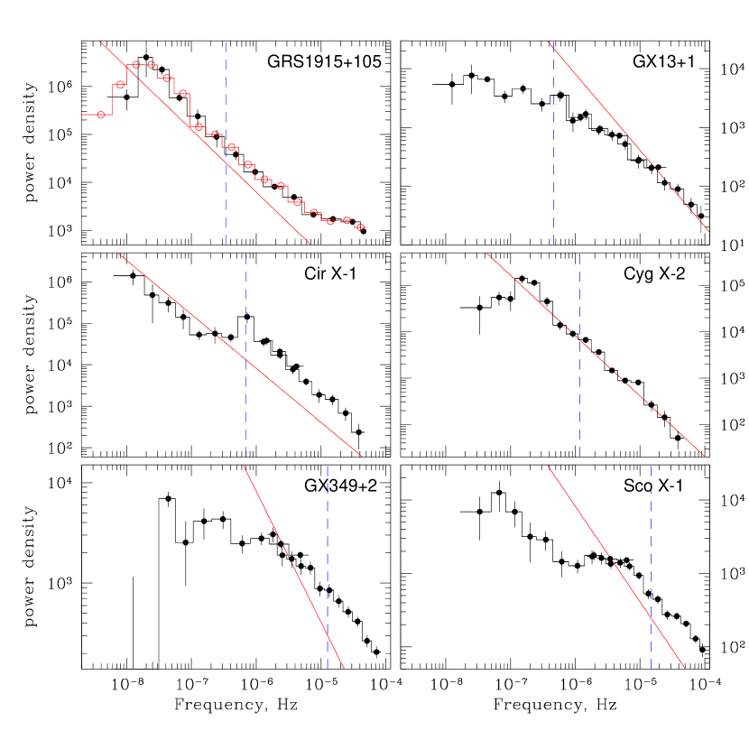
Figure 3: Power density spectra of LMXBs from the ASM sample. The solid line in each panel shows $P_{\nu}=1\cdot 10^{-4}\,\nu^{-1.3}$ power law. The vertical dashed line marks the orbital frequency. In the upper left panel the histogram marked with hollow circles without error bars shows the power spectrum of GRS1915+105 obtained from the entire ASM time series of duration $\approx 8$ years. Note that the vertical scale is different in different panels.

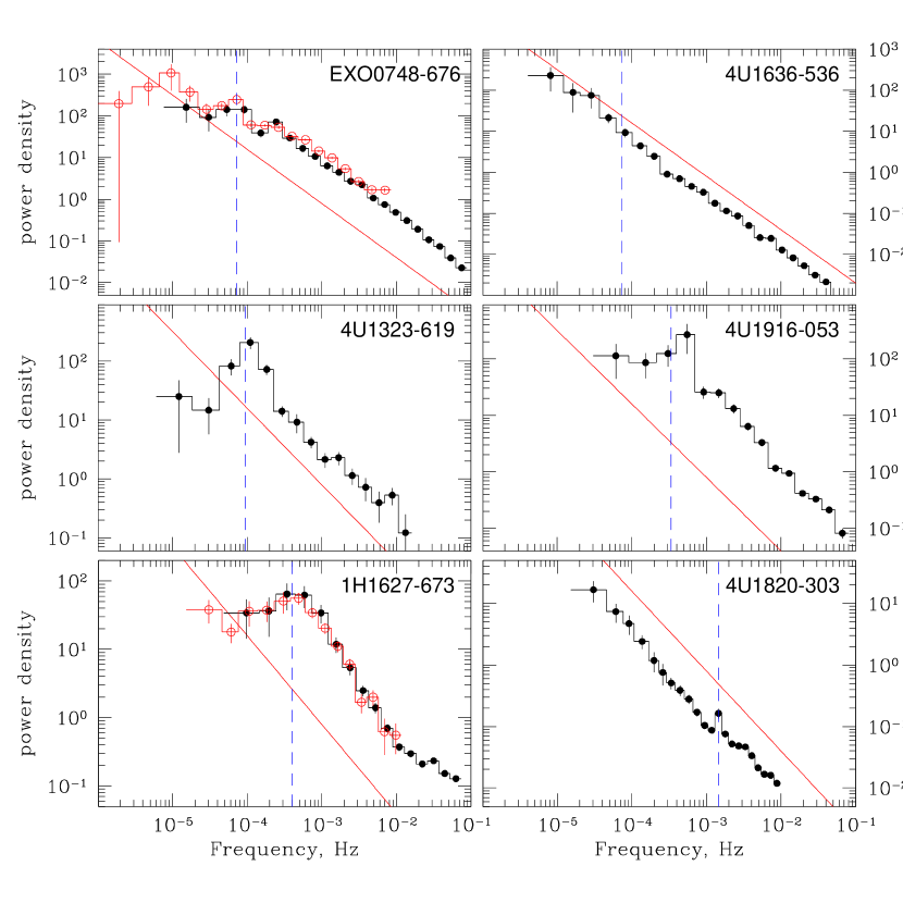
Figure 4: Power density spectra of LMXBs from the EXOSAT sample obtained from the ME data. The solid line in each panel shows $P_{\nu}=1\cdot 10^{-4}\,\nu^{-1.3}$ power law, the same as in Fig.3. The vertical dashed line marks the orbital frequency. For EXO0748–676 and 1H1627–673 the power spectra obtained from the GSPC data are also shown (histograms marked with hollow circles). Note that the vertical scale is different in different panels.

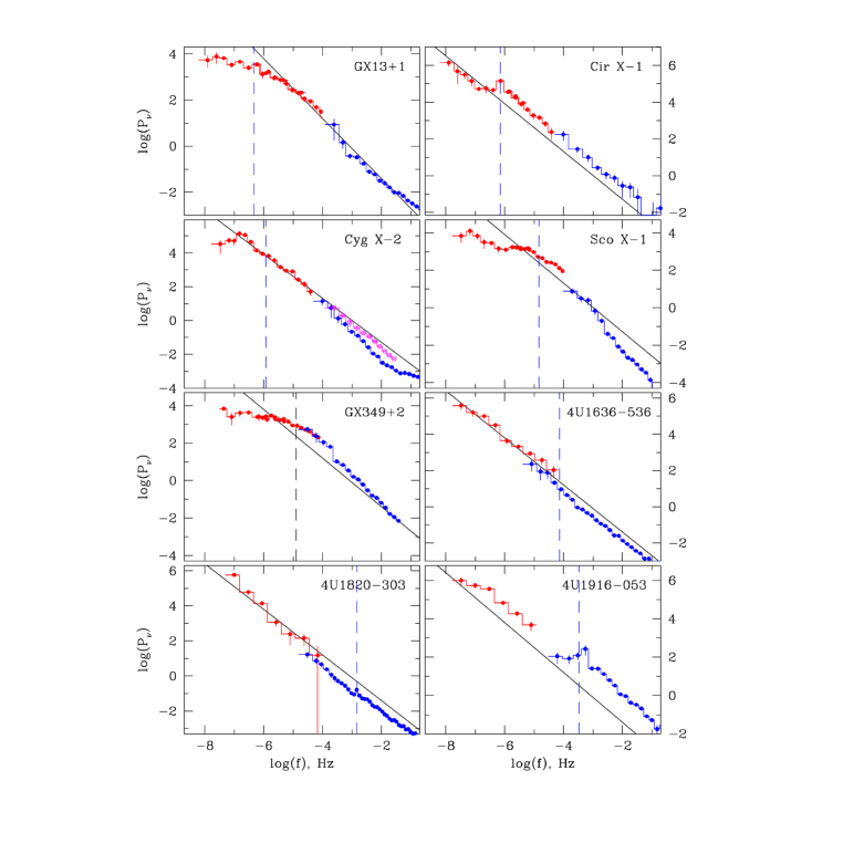
Figure 5: Broad band power spectra of LMXBs based on ASM and EXOSAT data. The solid line in each panel shows $P_{\nu}=1\cdot 10^{-4}\,\nu^{-1.3}$ power law, the same as in Fig.3 and 4. The vertical dashed line marks the orbital frequency. For Cyg X-2 the power spectrum obtained from the RXTE/PCA data is also shown (the histograms marked with open circles). Note that the vertical scale is different in different panels.

The power spectra of selected sources are shown in Figs.3 and 4. For reference, we plot in each panel a power law spectrum $P_{\nu}=1\cdot 10^{-4}\,\nu^{-1.3}$. Flattening at frequencies $f\ga 10^{-5}$ Hz can be seen in the PDS of GRS 1915+105. This can potentially be related to the specifics of ASM light curves, namely, it can be caused by the aliasing effect leading to the leakage of higher frequency power below the Nyquist frequency. The assessment of the reality of this flattening is beyond the scope of the present paper. Also seen for some sources (most prominently for Cir X-1 and 4U1820–303) are the peaks due to the orbital modulation. In Fig.5 we show combined power spectra based on the ASM and EXOSAT light curves. These spectra cover $\sim 10^{-8}-10^{-1}$ Hz frequency range. For several faint sources from the EXOSAT sample no meaningful power spectra can be obtained from the ASM light curves due to too low count rate. For GRS1915+105, obviously, no EXOSAT data exist.

The power spectra of almost all sources show a clear low frequency break, below which they are nearly flat. For some sources the second very low frequency component is present at lower frequencies. The most clearly this component can be seen in the case of Cir X-1, Sco X-1 and 4U1916–536. Some sources also show broad QPO like features near or below the break frequency. At high frequencies, above the break, the power spectra follow the $P_{\nu}\propto\nu^{-\alpha}$ power law. Remarkably, the slope of the power law appears to be similar in all 12 sources, $\alpha\sim 1.3$. The same is true for the normalization.

3.1 4U 1636-536 and 4U 1820-303

There is at least one exception from the above behavior. No evidence for break was found in the PDS of 4U 1636-536. Although the power spectrum of this source might have several weak features, its overall behavior in an extremely broad frequency range from $10^{-8}-10^{-1}$ Hz is well represented by the power law with slope $\alpha\approx 1.3$ and without any obvious break (Fig.5).

The second possible exception is 4U 1820-303. In addition to clearly visible peak due to the orbital modulations, it appears to have a shoulder at $f\sim 10^{-3}-10^{-2}$ Hz followed by a power law at lower frequencies. The presence of this shoulder is more obvious in the data of individual EXOSAT observations, shown in Fig.6. In the formal statistical sense the existence of the low frequency break is highly significant. For example, approximation of the Aug. 19–20, 1985 data in the $10^{-3}-2\cdot 10^{-2}$ Hz frequency range gave the following values: $\chi^{2}=12.7$ (11 d.o.f.) and $\chi^{2}=42.2$ (12 d.o.f.) for the power law model with and without low frequency break respectively, resulting in $\Delta\chi^{2}\approx 30$ for one additional parameter. However, considering the overall shape of the power spectrum (e.g. Fig.5), this source presents a less obvious case than the others in our sample.

Chou & Grindlay (2001) analyzing long term X-ray variability of 4U 1820-303 confirmed earlier suggestion that it is a hierarchical triple system, where ultra-close X-ray binary is orbited by companion with orbital period about 1.1 day. Due to influence of the third star the well-known 176 day X-ray modulation of 4U 1820-303 is generated. Influence of the third star can also give rise to very low frequency modulation of the mass transfer rate in this system, unrelated to the $\dot{M}$ variations intrinsic to the accretion disk. This could, in principle, explain strong very low frequency power law component at $f\la 10^{-3}$ Hz. In the following we associate the shoulder at $\log(f)\sim-2.5$ with the low frequency break similar to the ones observed in other LMXBs in our sample. We emphasize that this interpretation is not unique and 4U 1820-303, like 4U 1636-536, can show the behavior different from other sources in our sample.

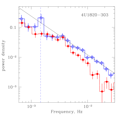
Figure 6: The power spectrum of 4U1820-303 obtained by EXOSAT on April 16 (open circles) and August 19–20 (filled circles), 1985. The solid line shows $P_{\nu}=3\cdot 10^{-5}\,\nu^{-1.3}$ power law. The vertical dashed line marks the orbital frequency.

3.2 PDS approximation

The power density spectra were approximated by a model of a power law with low frequency break:

$$P(f)=\left\{\begin{array}[]{ll}A\,f^{-\alpha}&\mbox{~{}~{}~{} $f\geq f_{\rm break}$}\\ A\,f_{\rm break}^{-\alpha}&\mbox{~{}~{}~{} $f<f_{\rm break}$}\end{array}\right.$$ (4)

An additional Lorentzian component was added to the model for the sources with strong orbital modulation and/or broad low frequency QPO peaks. The frequency range was chosen for each source individually, depending on the duration of the available time series and the presence of the additional noise component below $f_{\rm break}$. The adopted frequency ranges and best fit values of the model parameters are listed in Table 2, along with the count rates and X-ray luminosities of the sources. The large width of the QPO component present in the power spectra of several sources close to the low frequency end makes the determination of the break frequency somewhat ambiguous. For these sources (GRS1915+105, Cyg X-2 and 4U 1323–619) we list the values of the break frequency obtained with and without the Lorentzian component in the model. In the following the average of the frequencies of the two models are used. The statistical uncertainty of the break frequency in these sources are obtained from combined confidence intervals of the models with and without Lorentzian component. At least three harmonics of the orbital frequency are present in the power spectrum of 4U1323–619. The corresponding bins of the power spectrum were excluded from the fitting procedure.

Table 2: The parameters of power spectra approximation.

Source	ASM	EXOSAT	$L_{X}$	$f_{\rm break}$	$\alpha$	$f_{\rm QPO}$	$f$ range
	cnts/sec	cnts/sec	$10^{37}$ erg/s	Hz		Hz	Hz
	(1)	(2)	(3)	(4)	(5)	(6)	(7)
GRS 1915+105	60.7	—	34	$4.03_{-0.64}^{+1.07}\times 10^{-8}$	$1.32_{-0.09}^{+0.08}$	—	$5\cdot 10^{-9}-1\cdot 10^{-6}$
				$6.50_{-1.64}^{+2.78}\times 10^{-8}$	$1.26_{-0.11}^{+0.18}$	$2.8_{-2.8}^{+7.0}\times 10^{-8}$	$5\cdot 10^{-9}-1\cdot 10^{-6}$
GX 13+1	23.1	—	4.3	$1.13\pm 0.25\times 10^{-7}$	$0.56\pm 0.03$	—	$1\cdot 10^{-8}-1\cdot 10^{-5}$
Cir X-1	74.2	—	8.6	$1.14_{-0.18}^{+0.12}\times 10^{-6}$	$1.51\pm 0.13$	$7.26_{-0.84}^{+1.11}\times 10^{-7}$	$1\cdot 10^{-7}-1\cdot 10^{-5}$
Cyg X-2	37.9	—	7.5	$2.28_{-0.38}^{+0.15}\times 10^{-7}$	$1.26\pm 0.06$	—	$1\cdot 10^{-8}-1\cdot 10^{-5}$
				$3.66_{-1.47}^{+0.36}\times 10^{-7}$	$1.13\pm 0.09$	$1.87\pm 0.09\times 10^{-7}$	$1\cdot 10^{-8}-1\cdot 10^{-5}$
GX 349+2	51.6	—	16.7	$2.78_{-0.92}^{+0.63}\times 10^{-6}$	$0.66\pm 0.06$	—	$1\cdot 10^{-8}-1\cdot 10^{-5}$
Sco X-1	917	—	27.4	$6.14_{-0.71}^{+1.06}\times 10^{-6}$	$0.89_{-0.06}^{+0.10}$	—	$5\cdot 10^{-7}-5\cdot 10^{-5}$
EXO 0748–676	0.57	44.0	0.37	$1.03_{-0.12}^{+0.16}\times 10^{-4}$	$1.25\pm 0.01$	—	$1\cdot 10^{-5}-3\cdot 10^{-2}$
4U1636–536	14.7	153		—	$1.29\pm 0.01$	—	$1\cdot 10^{-5}-3\cdot 10^{-2}$
4U1323–619	0.60	4.4	0.14	$2.01\pm 0.22\times 10^{-4}$	$1.26_{-0.08}^{+0.10}$	—	$1\cdot 10^{-5}-3\cdot 10^{-2}$
				$2.10\pm 0.60\times 10^{-4}$	$1.21\pm 0.11$	$8.14_{-0.30}^{+0.36}\times 10^{-5}$	$1\cdot 10^{-5}-3\cdot 10^{-2}$
4U1916–053	1.0	17.8	0.26	$4.25_{-0.83}^{+1.22}\times 10^{-4}$	$1.41\pm 0.05$	—	$3\cdot 10^{-5}-3\cdot 10^{-2}$
1H1627–673	0.59	44.5	0.41	$5.78_{-1.25}^{+0.86}\times 10^{-4}$	$1.53\pm 0.08$	—	$4\cdot 10^{-5}-3\cdot 10^{-2}$
4U1820–303	19.8	368	3.4	$2.99_{-0.20}^{+0.21}\times 10^{-3}$	$1.43\pm 0.06$	—	$4\cdot 10^{-5}-3\cdot 10^{-2}$

(1), (2) – ASM and EXOSAT count rates; (3) – X-ray luminosity calculated using respective count rates and source distances listed in Table 1; (4) – break frequency; (5) – power law slope; (6) – the centroid frequency of the Lorentzian component; (7) – frequency range for PDS fits.

4 Viscous time scale in LMXBs

For the standard accretion disk (Shakura & Sunyaev, 1973) the viscous time scale at the outer edge of the disk $R_{d}$ can be estimated as:

$$t_{\rm visc}=\frac{2}{3\alpha}\,\left(\frac{H_{d}}{R_{d}}\right)^{-2}\frac{1}{\Omega_{K}(R_{d})}$$ (5)

where $R_{d}$ is the disk outer radius, $\Omega_{K}=\sqrt{GM_{1}/R_{d}^{3}}$ is the Keplerian frequency, $H_{d}$ is the disk half-thickness at the outer edge, $M_{1}$ is the mass of the primary and $\alpha$ is the dimensionless viscosity parameter.

Combining the eq.(5) with the third Kepler law:

$$P_{orb}=2\pi a^{3/2}[G(M_{1}+M_{2})]^{-1/2},$$ (6)

and assuming that the binary has a circular orbit one finds:

$$\frac{f_{\rm visc}}{f_{\rm orb}}=\frac{3\pi\alpha}{\sqrt{1+q}}\left(\frac{H_{d}}{R_{d}}\right)^{2}\left(\frac{R_{d}}{a}\right)^{-3/2}$$ (7)

where $q=M_{2}/M_{1}$ is the mass ratio, $a$ is binary separation, $f_{\rm orb}=1/P_{\rm orb}$ and $f_{\rm visc}=1/t_{\rm visc}$. From eq.(7) it follows that for fixed viscosity parameter and relative disk thickness and size, the viscous time scale is directly proportional to the orbital frequency of the binary system, as intuitively expected.

To estimate the expected range of values of $f_{\rm visc}/f_{\rm orb}$ one needs to know the disk size and thickness. The thickness of the standard Shakura–Sunyaev disk is

$$\frac{H}{R}\approx 1.9\cdot 10^{-2}\ \alpha^{-1/10}\ R_{\rm 10km}^{3/20}\ M_{1.4}^{-21/40}\ L_{37}^{3/20}\ R_{10}^{1/8}$$ (8)

where $M_{1}=1.4\,M_{1.4}$ is the mass of the compact object in solar units, $R_{0}=10^{6}\,R_{\rm 10km}$ cm is defined so that $L_{X}=GM_{1}\dot{M}/R_{0}$, $L_{X}=10^{37}\ L_{37}$ erg/s is X-ray luminosity, and $R_{d}=10^{10}\ R_{10}$ cm is the outer disk radius. The disk thickness predicted by this relation varies from $H/R\sim 0.02$ for the most compact and low luminosity systems to $H/R\sim 0.03-0.04$ for sources in the upper part of the Table 1. Irradiation of the disk by the X-rays from the vicinity of the compact object, although does increase significantly the surface temperature of the outer disk, has a little effect on its mid-plane temperature, due to large optical depth of the Shakura-Sunyaev disk (Lyutyi & Sunyaev, 1976). Correspondingly, account for irradiation effects does not change the above estimates significantly. With plausible values of two other parameters in eq.(7), $\alpha\approx 0.5$ and $R_{d}/a\approx 0.3-0.6$, the standard theory predicts:

$$\left(\frac{f_{\rm visc}}{f_{\rm orb}}\right)_{\rm std}\sim 0.005-0.07$$ (9)

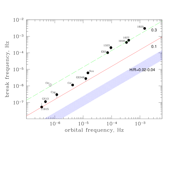
Figure 7: Relation between the PDS break frequency and the orbital frequency of the binary system. The shaded area shows the dependence $f_{\rm visc}$ vs. $f_{\rm orb}$ expected for the Shakura–Sunyaev disk, assuming $\alpha=0.5$, $\beta=f_{\rm break}/f_{\rm visc}=1$, $q=0.5$ and $R_{d}/a=0.4$. Straight solid and dashed lines are predictions for larger values of the disk thickness $H/R$, as indicated by the numbers on the plot. The two points for Cir X-1 correspond to the observed orbital period of $P_{\rm orb}\approx 16.6$ d (open circle) and corrected for the orbital eccentricity assuming $e=0.7$, as described in the section 4.2 (filled circle).

4.1 Break frequency

Power density spectra of all but one LMXBs from our sample have the low frequency break predicted in the simple qualitative picture outlined in the Introduction. Fig. 7 shows the dependence of the best fit value of the break frequency on the orbital frequency of the binary system. There is an obvious positive correlation between these two frequencies broadly consistent with eq.(7). Remarkably, this correlation holds over 3 order of magnitudes in the orbital frequency, from compact binaries 4U 1820-303 and 1H1627–673 with $P_{\rm orb}\approx 12$ and $\sim 40$ min to extremely wide system GRS 1915+105 with $P_{\rm orb}\approx 33.5$ days. The value of $f_{\rm break}/f_{\rm orb}$ ranges from $\sim 0.1-0.2$ for long period binaries to $\sim 1-2$ for the more compact ones. The broad band spectra shown in Fig.5 confirm that the breaks are indeed unique and well defined features in the power spectra.

In the following we assume that the break frequency corresponds to the viscous time scale of the accretion disk, and they are related by a simple linear relation:

$$t_{\rm visc}^{-1}=f_{\rm visc}=\beta^{-1}f_{\rm break}$$ (10)

Note that this simplified picture does not take into account complexity of the power density distribution near the viscous time scale.

With this definition the break frequency is related to the orbital frequency via:

$$\frac{f_{\rm break}}{f_{\rm orb}}=\beta\ \frac{3\pi\alpha}{\sqrt{1+q}}\left(\frac{H_{d}}{R_{d}}\right)^{2}\left(\frac{R_{d}}{a}\right)^{-3/2}$$ (11)

4.2 Cir X-1

Cir X-1 appears to deviate from the general trend in Fig.7, having the break/viscous time scale by a factor $\sim 10$ shorter than expected given its orbital period.

The significant orbital modulation of the X-ray activity suggests a highly eccentric orbit in this binary system (Murdin et al., 1980). Johnston et al. (1999) proposed a model, where the system consists of a neutron star on a highly eccentric, $e\sim 0.7-0.9$ orbit around a $\sim 3-5$ $M_{\odot}$ sub-giant companion. In this model the donor star fills its Roche lobe and the mass transfer occurs only during the periastron passage. Outside the periastron the donor star is detached from its Roche lobe surface and the mass transfer in the binary stops.

In such a system the disk radius would be defined, to first approximation, by the minimal separation between the components, $a_{\rm min}=(1-e)\ a$. As the eq.(7) was derived for a circular orbit, the following substitution should be made in interpreting the Cir X-1 data:

$$a\rightarrow a\ (1-e)\hskip 34.14322pt$$ (12)

$$P_{\rm orb}\rightarrow P_{\rm orb}\ (1-e)^{3/2}$$

Plotted in Fig.7 are two point for Cir X-1. The open circle corresponds to the observed orbital period of the source, the filled circle corresponds to the orbital period corrected for the eccentricity of the orbit assuming $e=0.7$. With this substitution the consistency with other sources is restored.

4.3 Viscous time and disk thickness

Although the break frequency does increase linearly with the binary orbital frequency, the ratio $f_{\rm break}/f_{\rm orb}\sim 0.2-2$ is notably larger than predicted for the Shakura-Sunyaev disk, $\left(f_{\rm visc}/f_{\rm orb}\right)_{\rm std}\sim 0.005-0.07$. The latter range of values is shown as the hatched area in the Fig. 7. Obviously, larger values of $f_{\rm visc}/f_{\rm orb}$ imply that the disk viscous time as traced by the position of the break on the PDS is by a factor of $\ga 5-10$ shorter than predicted by the theory. As it follows from eq.(7) and (11), there are several parameters affecting the disk viscous time, of which the strongest dependence is upon the disk size and thickness.

The theoretical and observational constrains on the disk size are summarized in Fig.8. It has two well known theoretical limits. Due to the angular momentum conservation, the disk radius can not be smaller than the circularization radius. The results of the numerical calculations of Lubow & Shu (1975) can be approximated by

$$\frac{R_{\rm circ}}{a}=0.074\ \left(\frac{1+q}{q^{2}}\right)^{0.24}$$ (13)

This approximation is accurate to $\approx 3\%$ in the range of the mass ratios $0.03\leq q\leq 10$. The upper limit on the disk size is given by the tidal truncation radius (Papaloizou & Pringle, 1977; Ichikawa & Osaki, 1994). In the case of small pressure and viscosity its value is close to the radius of the largest non-intersecting periodic orbit (Paczynski, 1977). The latter can be approximated by:

$$\frac{R_{\rm tidal}}{a}=0.112+\frac{0.270}{1+q}+\frac{0.239}{(1+q)^{2}}$$ (14)

accurate to $\approx 3\%$ in the range of $0.06\leq q\leq 10$. These two limits on the disk radius are shown as thick dash-dotted lines in Fig.8. On the observational side, there is a number of spectroscopic and photometric determinations of the disk radius in CVs (Hessman, 1988; Hessman & Hopp, 1990; Rutten et al., 1992; Harlaftis & Marsh, 1996; Harrop-Allin & Warner, 1996) and fewer in LMXBs (Orosz & Kuulkers, 1999; Shahbaz et al., 2004; Torres et al., 2004; Zurita et al., 2000). These data indicate (Fig.8) that for a steady disk the disk radius is close to the tidal truncation radius as defined by Paczynski (1977), with possible exception of the small-q systems (section 4.4).

With these values of the disk size and accepting $\alpha\sim 0.5$ as a plausible value of the viscosity parameter, the disk thickness of

$$H/R\ga 0.1\ \alpha_{0.5}^{-1/2}\beta^{-1/2}$$ (15)

is required in order explain observed values of the break frequency.

This conclusion relies on the association of the break in the power density spectra with the viscous time scale of the disk and as long as the assumption $\beta=f_{\rm break}/f_{\rm visc}\sim 1$ is valid, it is very robust. Indeed, in order to describe the data with $H/R\sim{\rm few\ \times\ }10^{-2}$, as predicted by the standard theory, one would need to increase dramatically the $\alpha$-parameter, up to implausibly high values of $\alpha\sim 5-800$. Alternatively, short viscous time of the disk could be achieved by reducing the Roche-lobe filling factor of the disk, down to $R_{d}/a\sim 0.005-0.05$. This is significantly smaller than the circularization radius and contradicts to both theoretical expectations and observations of the disks in CVs and LMXBs (Fig.8).

The latter possibility can be also interpreted that only the very inner part of the accretion disk, $R/a\sim 0.005-0.05$, contributes to the observed variability of LMXBs in X-rays. This can not be excluded a priori. We note however, that in this case the sharpness of the breaks observed in the power spectra of at least some sources (e.g. Sco X-1, EXO 0748–676, etc) implies that the transition from the (outer) region of negligibly small amplitude of the $\dot{M}$ perturbation to the (inner) region of relatively large ones should occur in a rather narrow range of radii.

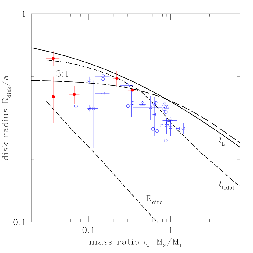
Figure 8: Theoretical and observational constrains on the disk radius. The solid curve shows the effective radius of the Roche lobe of the primary. Two dash-dotted curves show the circularization and tidal truncation radius. The dashed line is the radius of 3:1 tidal resonance. The open circles and triangles are measurements and lower limits for CVs in the outburst state. The small filled circles show the disk radius in LMXBs. The reference for these optical data are given in the text.

Figure 9: Dependence of the ratio $f_{\rm break}/f_{\rm orb}$ on the orbital period of the binary system (left) and its mass ratio (right).

4.4 Viscous time in wide and compact systems

As is evident from Fig.7, there is a significant dichotomy in the value of $f_{\rm break}/f_{\rm orb}$ ratio between long- and short-period binaries. This is further illustrated by Fig.9 where the ratio $f_{\rm break}/f_{\rm orb}$ is plotted against the binary orbital period and the mass ratio. The average values of $f_{\rm break}/f_{\rm orb}$ are $\approx 0.23$ and $\approx 1.7$ for the wide and compact systems correspondingly. The sense of the difference is that the compact systems have systematically shorter, by a factor of $\sim 8$, viscous time expressed in the orbital periods than the wide ones, the boundary lying at $P_{\rm orb}\sim 10$ hours or $q\sim 0.3$. The fact that this bimodality occurs between compact and wide systems or, equivalently, (with the exception of GRS1915+106) between small- and large-q binaries suggests that it may be caused by the excitation of tidal resonances in the accretion disk.

The phenomenon of tidal resonances in accretion disks is well studied in the context of dwarf novae (Whitehurst, 1988; Whitehurst & King, 1991; Lubow, 1991). The resonance occurs if the angular frequency of the orbital motion of the particle in the disk is commensurate with the angular frequency of the orbital motion of the secondary. For a Keplerian disk, the location of the resonant orbits is given by

$$\frac{R_{\rm res}}{a}=\left(\frac{k}{m}\right)^{2/3}\,(1+q)^{-1/3}$$ (16)

where $k,m$ are integers (e.g. Whitehurst & King, 1991). An obvious condition for a resonance being excited is that this radius lies within the accretion disk. From analytical studies and numerical simulations it is known that the strongest resonance occurs at the lowest order commensurability, $\Omega_{\rm K}:\Omega_{\rm orb}=2:1$ (e.g. Whitehurst & King, 1991). However the 2:1 resonant radius lies within the accretion disk only at extreme values of the mass ratio, $q\la 10^{-2}$. The next strongest resonance, most important in the context of binaries with not too extreme values of the mass ratio lies at the 3:1 commensurability. The higher order resonances are probably not excited in the accretion disks. The dependence of the 3:1 resonance radius on the mass ratio $q$ is shown by the dashed line in Fig.8, confirming the well known fact that the $3:1$ resonance can be excited in the systems with the mass ration $q\la 0.3-0.4$. Note that the precise value of the threshold $q$ depends on the definition of the tidal truncation radius, due to small angle between the two curves in Fig.8. Under the assumption that $R_{\rm tidal}=0.9R_{L}$ it is $q\approx 0.33$. With the definition of $R_{\rm tidal}$ used in Fig.8 the threshold value is slightly larger.

Numerical simulations of the non-linear stage of the instability have shown that excitation of tidal resonances results in a significant asymmetry of the accretion disk and causes its precession in the reference frame of the binary (Whitehurst, 1988; Whitehurst & King, 1991; Lubow, 1991). Additionally, the accretion disk is truncated near the resonant radius. This explains the values of the disk radii smaller than the tidal truncation radius observed in CVs and LMXBs with small mass ratios (Fig.8).

To conclude, with exception of GRS1915+105, discussed in section 5.2.1, the excitation of the 3:1 inner Lindblad resonance provides a natural explanation of the dichotomy in the viscous time scale between wide and compact systems.

5 Discussion.

5.1 Thickness of the disk

5.1.1 Semi-thick disk or coronal flow?

The values of the viscous time scale of the disk inferred by the position of the low frequency break in the power spectra of LMXBs require rather large disk thickness, $H/R\ga 0.1\ \alpha_{0.5}^{-1/2}\beta^{-1/2}$, by a factor of $\ga 3-5$ exceeding the prediction of the standard theory of the accretion disks. Taken at the face value, $H/R\ga 0.1$ appears to agree with the statistics of the eclipsing systems among LMXBs (e.g. Milgrom, 1978; Narayan & McClintock, 2004). However, large values of $H/R$ result in small optical depth of the outer disk, which is inconsistent with numerous observations of the optical emission from accretion disks, as discussed below.

We consider the structure of an accretion disk with some value of the vertical scale-height $H/R\sim 0.1$, without specifying the source of the additional energy dissipation. Under the assumption of vertical hydrostatic equilibrium and stationarity, both the mid-plane disk temperature and the density are steep functions of the disk thickness: $T/T_{\rm vir}\propto(H/R)^{2}$, $\rho\propto(H/R)^{-3}$. Due to strong dependence of the Rosseland mean opacity on the density and temperature, typically as $k_{R}\propto\rho^{\approx 1}\,T^{\approx-3.5}$ in the parameters range of interest, the optical depth of the disk $\tau_{R}=k_{R}\rho H$ is also steeply decreasing function of the disk thickness, $\tau_{R}\propto(H/R)^{-\gamma}$ with the power law index $\gamma$ changing from $\sim 12$ to $\sim 3$ as the $H/R$ increases (Fig.10). Therefore, even a moderate increase of the disk thickness would lead to dramatic decrease of its optical depth. As a result, for $H/R\sim 0.1$, the accretion disk in the majority of LMXBs from our sample would be optically thin. This would contradict to a number of observational facts, mostly from the optical band, proving existence of the optically thick outer disk in LMXBs. Indeed, the free-free optical depth in the optical V-band equals

$$\tau_{ff}({\rm V-band})\approx\hskip 156.49014pt$$ (17)

$$3.8\cdot 10^{-2}\ln\left(\frac{T}{5500\rm~{}K}\right)\dot{M}_{17}^{2}\,M_{1.4}^{-5/2}\,\alpha_{0.5}^{-2}\,\left(\frac{H}{R}\right)_{0.1}^{-8}R_{10}^{-1/2}$$

where $(H/R)_{0.1}$ is the disk geometrical thickness normalized to 0.1. The above approximation is accurate to $\sim 10\%$ in the $10^{4}\leq T\leq 10^{8}$ K temperature range, the logarithmic term due to the Gaunt factor varies from 2.9 to 7.5 for the temperature in the range $10^{5}-10^{7}$ K. For the parameter of binaries from our sample the optical depth in the V-band would be $\tau_{ff}\ll 1$, with the exception of sources with the largest $\dot{M}$ (Sco X-1, GX349+2 and 4U1820) where $\tau_{ff}\sim 1-10$. The low optical depth in the V-band would conflict with numerous spectroscopic observations of the optical emission from the LMXBs, suggesting existence of the continuum emission originating from the optically thick outer accretion disk (e.g. Hynes et al., 2002; Chaty et al., 2003). On this basis the possibility of the semi-thick, $H/R\sim 0.1$ outer disk in LMXBs can be excluded.

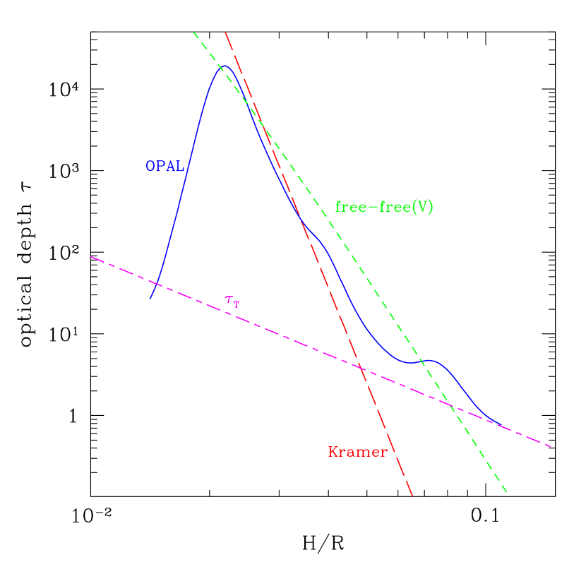
Figure 10: Dependence of optical depth of the disk at $R=5\cdot 10^{10}$ cm on the $H/R$ ratio for $\dot{M}=5\cdot 10^{17}$ g/s, $M=1.4$ $M_{\odot}$, $\alpha=0.5$. The solid line shows the optical depth based on the OPAL opacities (Iglesias & Rogers, 1996), long dashed line – Kramer law ($k_{R}=5\cdot 10^{24}\,\rho\,T^{-7/2}$ cm²/g), short dashed – free-free absorption in the optical V-band, dash-dotted – Thompson optical depth.

Instead, one can envisage a two phase accretion flow with a Shakura-Sunyaev-like disk in the mid-plane surrounded by the tenuous optically thin coronal flow with the aspect ratio $H/R\sim 0.1-0.2$ and temperature of $T\sim 10^{-2}\,T_{\rm vir}$. In order to explain the prominence of the low frequency break in the power spectrum, a significant fraction of the accretion has to take place in this corona

$$\dot{M}_{\rm corona}\sim\dot{M}_{\rm disk}$$ (18)

The temperature and density in the coronal flow are:

$$T\approx 1.4\cdot 10^{5}\ M_{1.4}\,\left(\frac{H}{R}\right)_{0.1}^{2}R_{11}^{-1}{\rm~{}~{}[K]}$$ (19)

$$n\approx 3.6\cdot 10^{13}\ f_{c}\,\dot{M}_{17}\,M_{1.4}^{-1/2}\,\alpha_{0.5}^{-1}\left(\frac{H}{R}\right)_{0.1}^{-3}R_{11}^{-3/2}{\rm~{}~{}[cm^{-3}]}$$ (20)

where $f_{c}=\dot{M}_{\rm corona}/\dot{M}$. As the surface mass density depends on the thickness of the disk as $\Sigma\propto(H/R)^{-2}$, such a corona will contain a small fraction of the mass of the accreting matter:

$$\frac{\Sigma_{\rm c}}{\Sigma_{\rm d}}\sim\frac{f_{c}}{1-f_{c}}\,\left(\frac{H_{c}}{H_{d}}\right)^{-2}\la 10^{-1}$$ (21)

assuming $fc\sim 0.5$.

The vertical and radial column density of the coronal flow are $[cm^{-2}]$:

$$n\,H\approx 3.6\cdot 10^{23}\ f_{c}\,\dot{M}_{17}\,M_{1.4}^{-1/2}\,\alpha_{0.5}^{-1}\left(\frac{H}{R}\right)_{0.1}^{-2}R_{11}^{-1/2}$$

$$n\,R\approx 3.6\cdot 10^{24}\ f_{c}\,\dot{M}_{17}\,M_{1.4}^{-1/2}\,\alpha_{0.5}^{-1}\left(\frac{H}{R}\right)_{0.1}^{-3}R_{11}^{-1/2}$$ (22)

The plausible mechanism of formation of the coronal flow is the disk evaporation process originally proposed by Meyer & Meyer-Hofmister (1994) for dwarf novae. In X-ray binaries the physics of the disk evaporation is significantly affected by the illumination and Compton heating and cooling of the disk-corona system by the X-ray emission produced in the vicinity of the relativistic object. Although the the self-consistent treatment of the problem is yet to be done, the likely net effect of the X-ray irradiation is to increase the fraction of $\dot{M}$ in the coronal flow (Meyer et al., 2000; Jimenez-Garate et al., 2002, F.Meyer, private communication).

5.1.2 Other evidence of the coronal flow

An independent evidence of the existence of a diffuse ionized gas above the accretion disk plane is provided by observations of LMXBs with high inclination – the ADC sources and dippers. Based on observations of partial X-ray eclipses in 4U1822–371, White et al. (1981) concluded that the compact X-ray source in this system is diffused by a large moderately Compton thick highly ionized corona located above and below the accretion disk. Detailed modeling of the eclipse light curves in the ADC sources 4U1822–371 and 4U2129+47 (White & Holt, 1982) yielded estimates of the radial extent of the accretion disk corona in these sources, $R_{c}\sim(1-2)\cdot 10^{10}$ cm and $R_{c}\sim(3-6)\cdot 10^{10}$. These numbers are comparable with the value of the tidal radius in the systems, $R_{\rm tidal}\sim 3.9\cdot 10^{10}$ cm. The partial nature of the eclipses in these sources, with the eclipsed flux at the level of $\sim 50\%$ of the uneclipsed value indicated that the corona had non-negligible radial optical depth, $\tau_{T}\sim 1$, in agreement with the estimate of eq.(22).

High resolution spectroscopic observations of LMXBs with Chandra and XMM-Newton gratings are revealing complex absorption/emission features in their X-ray spectra (Cottam et al., 2001; Jimenez-Garate et al., 2003; Kallman et al., 2003; Boirin et al., 2004). These features are mostly pronounced in the systems with high binary inclination angle and suggest the presence of tenuous photo-ionized plasma orbiting the compact object above the orbital plane of the binary.

From the analysis of the recombination emission lines of H- and He-like ions of O, Ne and Mg in EXO0748–676 Jimenez-Garate et al. (2003) constrained the density and radial extend of the photoionized plasma, $N_{e}\sim 10^{12}-10^{15}$ cm^-3, $7\cdot 10^{9}\la R\la 6\cdot 10^{9}$ cm and the temperature $T\la 2\cdot 10^{5}$ K. This range of the parameters is consistent with the numbers computed from the above formulae for EXO0748–676 and assuming the aspect ratio of the coronal flow $H/R=0.1$: the tidal truncation radius $R_{\rm tidal}\sim 4.8\cdot 10^{10}$ cm, density in the coronal flow $N\sim 2.7\cdot 10^{13}f_{c}$ cm^-3, and temperature of $T\sim 3\cdot 10^{5}$ K.

Based on the observations of the narrow absorption lines of the H- and He-like Fe in the spectrum of 4U1916–053, Boirin et al. (2004) estimated the ionization parameter and the column density of the absorbing gas: $\log(\xi)\approx 3.9$, $NH\sim 2\cdot 10^{22}$ cm^-2. From these numbers one can estimate the radial extent and the density of the absorbing gas, $R\sim 1.6\cdot 10^{10}$ cm, $N\sim 1.3\cdot 10^{12}$ cm^-3. The tidal radius in this system is $\approx 2\cdot 10^{10}$ cm, in agreement with the value derived from the XMM-Newton data. The density in the coronal flow with $H/R=0.1$ is $N\sim 6.7\cdot 10^{12}f_{c}$ cm^-3. The latter number is somewhat larger than derived from the XMM-Newton data. This can be explained by smaller inclination angle in this source resulting in lower density along the line of sight. Indeed, unlike EXO0748–676 showing deep X-ray eclipses, 4U1916–053 shows only X-ray dips.

5.1.3 $\dot{M}$ variations due to geometrically thin disk

In this picture, the $\dot{M}$ variations in the geometrically thin Shakura–Sunyaev disk should give rise to the second very low frequency power law component, revealing itself below the break frequency. Such power law component is indeed observed in the power spectra of some of the sources. Most obvious its presence is in Cir X–1 and 4U1916–053 and, to less extent, in Sco X–1 (Fig.5). Remarkably, the slope of the power spectrum before and after the break are very similar, suggesting similar nature of the processes causing the variability. Furthermore, the second break should be expected at the low frequencies, corresponding to the (larger) viscous time of the geometrically thin disk. The frequency of the second break is described by eq.(11) with the $H/R$ given by eq.(8). An evidence of the second break may be seen in the power spectra of Sco X-1 and, possibly, of 4U1916–053. In the former case the break frequency equals $f_{\rm break}^{(2)}=8_{-4}^{+7}\cdot 10^{-8}$ Hz and the ratio $f_{\rm break}^{(2)}/f_{\rm orb}=5_{-3}^{+5}\cdot 10^{-3}$. This value is within the range predicted for standard Shakura–Sunyaev disk with the aspect ratio of $H/R\sim{\rm few}\cdot 10^{-2}$, eq.(9). The value of the break frequency in the case of 4U1916–053 is probably $f_{\rm break}^{(2)}\sim 10^{-7}$ Hz, although this number is less secure than that for Sco X-1. If correct, this is significantly, by $\sim 2-3$ dex smaller that expected in the above scenario.

In the conclusion of this section we note that due to power law dependence of the viscous time scale on the disk radius, $t_{\rm visc}\propto r^{3/2}$, the radial drift velocity of the matter in the accretion flow should be increased throughout the most ($\sim 80-90\%$) of the radial extent of the accretion disk. Therefore the bulge at the outer edge of the disk, resulting from the disk–stream interaction (e.g. Hellier & Mason, 1989) is insufficient as it is located at the outer edge of the disk. For the same reason this analysis based on the viscous time of the disk probes the outer disk and is insensitive to the conditions in its innermost parts, e.g. $R\la 10^{4}R_{g}$, which contribution to the total viscous time is negligibly small.

5.2 Tidal resonances and viscous time scale of the disk

The dichotomy in the viscous time between long- and short-period systems is naturally explained by excitation of the 3:1 inner Lindblad resonance. This suggestion is supported by detection of superhumps in several LMXBs with small mass ratios (e.g. Haswell et al., 2001; Zurita et al., 2002). Importantly, the superhumps are detected not only in transient sources but also in one or two persistent LMXBs, including one source from our sample, 4U1916–053 (Callanan et al., 1995).

The specific mechanism by which the tidal instability is affecting the viscous time of the disk is, however, unclear. It is also unclear if the coronal flow in the small-q system has indeed $H/R\sim 0.3$ and $T\sim 0.1\,T_{\rm vir}$ as it is formally required by the observed $t_{\rm visc}\sim P_{\rm orb}$. Several possibilities can be mentioned:

1. mass transfer in tidal waves excited in the disk by the tidal forces. It has been shown theoretically and confirmed in numerical simulations, that in the non-linear regime strong tidal waves are excited in the accretion disk (Spruit et al., 1987; Lubow, 1991; Truss et al., 2002). These waves, propagating in the disk with the speed significantly exceeding the radial drift velocity of the matter, can decrease the effective viscous time scale. If correct, the aspect ratio and coronal temperature in the small-q systems may be not significantly different from those in the large-q ones.

2. heating of the outer disk due to resonant tidal interaction (Whitehurst & King, 1991; Truss et al., 2002) can increase the temperature of the disk and/or coronal flow and, correspondingly, decrease the viscous time scale. As was mentioned above, in order to explain the observed viscous time scale the coronal flow temperature of $T\sim 0.1\,T_{\rm vir}$ is required.

3. non-trivial definition of the viscous time for an eccentric and precessing disk. In the fully developed instability the particles in the disk move on non-circular trajectories with large eccentricity. Therefore, the average velocity of the radial drift of the disk particles can be significantly different from the value predicted by the standard disk theory for a circular Keplerian disk.

We note, that the truncation of the accretion disk at the 3:1 resonance radius (Fig.8) can be excluded as the cause of the shorter viscous time scale in the small-$q$ systems, because the change of the outer disk radius by a $\la 20-30\%$ is insufficient to explain the observed decrease of the viscous time by the factor of $\sim 10$.

5.2.1 Case of GRS1915+105

GRS1915+105 clearly stands out among other small-q systems (Fig.9, right panel). Although it has small mass ratio, $q=0.058\pm 0.033$ (Harlaftis & Greiner, 2004), its ratio $f_{\rm break}/f_{\rm orb}$ is close to the value found in the binaries with $q\ga 0.3$. The most plausible explanation of such behavior is related to the transient nature of the source. We outline two possibilities:

1. the tidal instability is known to have a rather long growth time, of the order of $\ga 10^{2}$ binary orbital periods (e.g. Whitehurst, 1988). For GRS1915+105 $P_{\rm orb}\approx 33.5$ days and $10^{2}P_{\rm orb}$ corresponds to $\sim 10$ years. Therefore the time passed since the onset of the outburst ($\sim 10$ years) was insufficient for the tidal instability to fully develop. In this scenario one would expect an increase of the break frequency in the course of the outburst, unless the instability growth time is significantly longer than $\sim 10$ years. However, no statistically significant difference in the break frequency has been found between the first and second halves of the data. This fact speaks against the above suggestion.

2. due to the large size of the system ($\sim 8\cdot 10^{12}$ cm), the irradiation effects are insufficient to ionize the outer disk in GRS1915+105 which is in the cold, low-viscosity state (H.Ritter, private communication). Therefore its outer boundary is located near the circularization radius rather than has expanded to the tidal radius, as is the case for the persistent sources. Therefore there is no accretion disk at the 3:1 resonance radius (Fig.8) and the tidal instability is not excited. In this respect the present outburst of GRS1915+105 might be similar to normal outbursts in dwarf novae. As well known, for the same reason the superhumps in dwarf novae are observed (tidal instability is excited) only in during the superoutbursts but not during the normal outbursts (e.g. Osaki & Meyer, 2003).

5.3 Broad low frequency QPO features

For several sources broad QPO-like features are obvious in the power density spectra. Most apparent these features are in the case of Cyg X-2 and GRS1915+105 (Fig.3, 4). Among plausible mechanisms of appearance of quasi periodic variability in X-ray binaries on these time scales are the radiation-driven warping and precession of the accretion disk (e.g. Maloney, Begelman & Pringle, Maloney et al.1996) and mass-flow oscillations caused by diffusion instability (Meyer & Meyer-Hofmister, 1990). Both types of oscillations are caused by the irradiation of the accretion disk by the primary and their characteristic time scale is of the order of the viscous time scale of the disk. Accordingly, these features should appear near the break frequency in the power density spectrum.

Another possible mechanism of appearance of broad low frequency QPOs near the viscous frequency of the disk was suggested by Vikhlinin, Churazov & Gilfanov (1994). This mechanism is related to the anti-correlation of the $\dot{M}$ perturbations in the accretion flow on the time scales $t\sim t_{\rm visc}$. The anti-correlation appears in the presence of the steady mass supply through the outer boundary of the accretion flow and is a direct consequence of the energy conservation law. In this respect the broad QPO features observed near the viscous time scale of the outer disk might be similar to the broad QPOs detected near the high frequency break of power density spectrum of Cyg X-1 in the hard state, at frequency of $\sim 0.04-0.07$ Hz (Vikhlinin et al., 1994). In the latter case the values of the break frequency and of the QPO centroid frequency are defined by the viscous time scale of the inner hot flow, $R\la 10^{2}$ R_g, responsible for the production of the hard Comptonized emission in the low spectral state of black hole candidates.

6 Summary

We studied the low frequency variability of low mass X-ray binaries in order to search for the signatures in their power density spectra related to the viscous time scale of the disk. Our results can be summarized as follows:

1. As the viscous time is the longest time scale of the accretion disk, the $\dot{M}$ variations produced in the disk due to various instabilities should become independent of each other on the time scales longer than the viscous time, i.e. $\left<\dot{M}(t)\dot{M}(t+\tau)\right>\rightarrow 0$ at $\tau\ga t_{\rm visc}$ Correspondingly, the power density of $\dot{M}$ perturbations produced in the disk and of the observed X-ray flux variations should become independent of the frequency at $f\la t_{\rm visc}^{-1}$.

2. Using archival data of RXTE/ASM and EXOSAT/ME we studied X-ray variability of persistent LMXBs in the $f\sim 10^{-8}-10^{-1}$ Hz frequency range. In power density spectra of 11 sources out of 12 satisfying our selection criteria, we found a very low frequency break. The spectra approximately follow $P_{\nu}\propto\nu^{-1.3}$ power law above the break and are nearly flat below the break (Figs. 3–5). In some cases (Sco X-1, Cir X-1 and 4U1916–053) a second power law component with the same slope appears at $f\ll f_{\rm break}$.

3. In a very broad range of binary periods, from $P_{\rm orb}\sim 11$ min in ultracompact binary 4U1820-303 to $P_{\rm orb}\sim 33.5$ days in GRS1915+105, the break frequency correlates with the orbital frequency $f_{\rm orb}=1/P_{\rm orb}$ of the binary system (Fig.7), in good agreement with the theoretical prediction for the viscous frequency $f_{\rm visc}=t_{\rm visc}^{-1}$ (eq.7)

4. Assuming that the low frequency break is associated with the viscous time scale of the disk, $f_{\rm break}\sim 1/t_{\rm visc}$, the measured values of the break frequency imply that the viscous time of the disk is by a factor of $\ga 10$ shorter than predicted by the standard theory (section 4.3, Fig.7). Taken at the face value, this requires the relative height of the outer disk $H/R\ga 0.1$. Motivated by the low vertical optical depth of such semi-thick accretion flow we propose instead, that significant fraction of the accretion occurs through the coronal flow above the standard geometrically thin Shakura-Sunyaev disk (section 5.1.1, Fig.10). The aspect ratio of the coronal flow, $H/R\ga 0.1$, corresponds to the gas temperature of $T\ga 0.01\,T_{\rm vir}$. The corona has moderate optical depth in the radial direction, $\tau_{T}\sim 1$, and contains $\la 10\%$ of the total mass of the accreting matter. The estimates of the temperature and density of the corona are in quantitative agreement with the parameters inferred by the X-ray spectroscopic observations by Chandra and XMM-Newton of complex absorption/emission features in the LMXBs with large inclination angle.

5. We found a clear dichotomy in the $f_{\rm break}/f_{\rm orb}$ between wide and compact system, the accretion flow in the compact systems having $\sim 10$ times shorter viscous time expressed in the orbital periods of the binary, than in the wide ones (Fig.9). The jump in the $t_{\rm visc}/P_{\rm orb}$ ratio occurs at the binary system mass ratio of $q\sim 0.3$. This strongly suggests that the dichotomy between small-q and large-q systems is caused by the excitation of the 3:1 Lindblad resonance in the small-q systems (section 4.4).

7 Acknowledgments

We are grateful to Friedrich Meyer and Hans Ritter for numerous discussions of the physics of the accretion disks and superhumps phenomenon in dwarf novae. VA would like to acknowledge the partial support from the President of RF grant NS-2083.2003.2 and from the RBRF grant 03-02-17286. This research has made use of data obtained through the High Energy Astrophysics Science Archive Research Center Online Service, provided by the NASA/Goddard Space Flight Center.

Appendix A Power spectra from the the ASM data

To calculate power density spectra from ASM light curves we used the method based on the auto-correlation function (cf. Edelson & Krolik, 1988).

We begin with consideration of the equally spaced data. The measured time series is $x_{k}$ and equals the number of counts detected in the $k$-th time bin corresponding to the time interval of $t=(k-1)\Delta t\div k\Delta t$, where index $k$ runs from 0 to $N-1$, N is assumed to be even. The discrete Fourier transform of the time series is defined as :

$$\hat{x}_{j}=\sum^{N-1}_{k=0}\,x_{k}\,\exp\left(i\frac{2\pi jk}{N}\right)$$ (23)

where $j$ changes in the range $1\div N/2$. The power density in the $j$-th frequency bin, which center is $f_{j}=j/T$ Hz, expressed in units of rms²/Hz (rms is fractional rms of variability) equals:

$$P_{j}=\frac{2|\hat{x}_{j}|^{2}}{N_{\rm ph}}\,\frac{1}{\left<r\right>}=\frac{2|\hat{x}_{j}|^{2}}{\left<r\right>^{2}T}$$ (24)

where $N_{\rm ph}=\sum^{N-1}_{k=0}\,x_{k}$ is the total number of counts in the time series, $T=N\Delta t$ is its total duration and $\left<r\right>=N_{\rm ph}/T$ is the average count rate.

Combining eqs.23 and 24 one finds

$$P_{j}=\frac{2}{\left<r\right>^{2}T}\left(A_{0}\,N+2\sum_{l=1}^{N-1}(N-l)\left<A_{l}\right>\cos\frac{2\pi jl}{N}\right)$$ (25)

where $\left<A_{l}\right>$ is discrete auto-correlation function:

$$\left<A_{l}\right>=\left<x_{k}\,x_{k+l}\right>$$ (26)

The eq.25 expresses the well known fact that power equals the cosine transform of the auto-correlation function. The noise level in the power density spectrum equals:

$$P_{\rm noise}=2\,\frac{\sum_{k=0}^{N-1}\sigma_{k}^{2}}{\left<r\right>^{2}T}$$ (27)

where $\sigma_{k}$ is the error of $x_{k}$. For Poisson errors in $x_{k}$, $\sigma_{k}^{2}=x_{k}$ and $P_{\rm noise}=2/\left<r\right>$, in agreement with the conventional form (e.g. Leahy et al., 1983).

The ASM time series consists of the count rate measurements $r_{k}$, [cnts/sec], at unevenly spaced moments $t_{k}$, $k=1,...,N_{\rm ASM}$. The values of $r_{k}$ are averaged over the time interval ($\sim 90$ sec) much shorter than the distance between adjacent bins ($\sim 90$ min). As before, the auto-correlation function $A_{l}$ is defined on the grid of $N$ time bins, with the $k$-th bin corresponding to the time interval $t=(k-1)\Delta t\div k\Delta t$, where index $k$ runs from 0 to $N-1$. The $\left<A_{l}\right>$ is computed as

$$\left<A_{l}\right>=\left<(r_{i}-\left<r\right>)(r_{j}-\left<r\right>)\right>\,\Delta t^{2}$$ (28)

where the averaging is performed over all pairs $(i,j)$, $i>j$, for which $\Delta t_{ij}=t_{i}-t_{j}$ falls in the $l$-th time bin of the grid.

The time interval $\Delta t$ and the duration of the time series $T=N\Delta t$ are parameters of the transformation and define the frequency range covered by the output power density spectrum. Their choice depends on the effective Nyquist frequency of the time series and its duration. Appropriate for the parameters of the ASM light-curves are the following values: $\Delta t\sim 5\cdot 10^{3}\div 10^{4}$ sec and $T\sim 10^{7}\div 10^{8}$ sec. Advantage of this method is that the correctness of the chosen values of $\Delta t$ and $T=N\Delta t$ can be easily checked using the number of pairs $(i,j)$ used to compute the autocorrelation value at the given time scale $l\Delta t$ and the uniformity of these numbers across the full range of the time scales, from $\Delta t$ to $T=N\Delta t$.

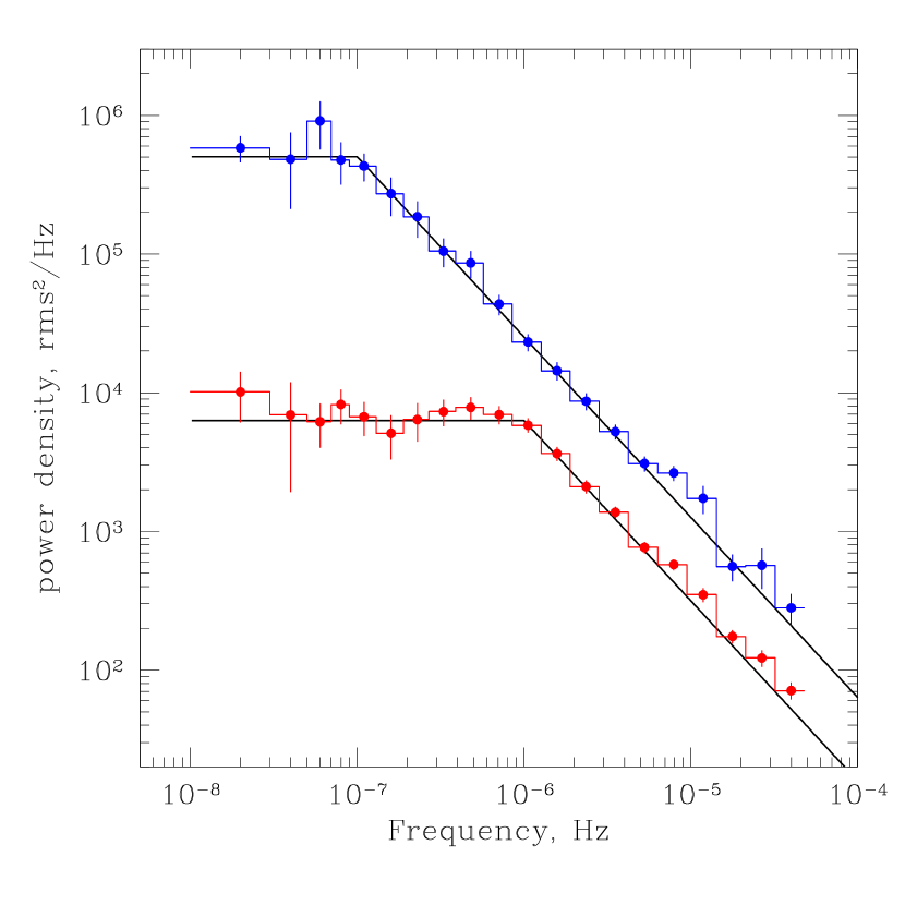
Figure 11: Results of simulations. The power density spectra of ASM light-curves simulated as described in the text. The solid lines show the model power density spectra used to generate faked ASM light curves: power law $P_{\nu}=10^{-4}f^{-1.3}$ with low frequency break at $10^{-6}$ and $10^{-7}$ Hz. The model with $f_{\rm break}=10^{-7}$ Hz and corresponding power density spectrum are shifted upwards by the factor of 4 for clarity.

With the auto-correlation computed according to eq.28, the power density spectrum can be easily computed using eq.25. As usual in the time series analysis, the entire time series is divided into $n$ segments and the power spectrum is computed for each segment separately. Their average and dispersion give estimates of the average power density spectrum and its uncertainty (under the assumption of stationarity).

If the errors for $r_{k}$ are known, the noise level in the output power spectrum can be computed as

$$P_{\rm noise}=2\,\frac{\sum_{k=1}^{N_{\rm ASM}}\sigma_{k}^{2}\,\Delta t}{\left<r\right>^{2}N_{\rm ASM}}$$ (29)

where $\sigma_{k}$ is the error of $r_{k}$ (in units of cnts/sec) and $N_{\rm ASM}$ is the number of ASM measurements used to compute one power spectrum. In practice, the flux measurement errors given in the ASM light-curves are slightly underestimated, therefore the noise level computed with eq.29 is somewhat imprecise (Grimm et al., 2002).

The performance of the method described above was verified in simulations. The initial light curve with the time resolution of $\sim 100$ sec was computed assuming the power law spectrum with slope of 1.3 and low frequency break at $f=10^{-6}$ Hz and $f=10^{-7}$ Hz and random Fourier phases. From this light curve the ASM time series was simulated using the measurements times $t_{k}$ of the real ASM light curve of Cyg X-2. The obtained light curve was randomized assuming Gaussian errors with the standard deviation equal the real ASM measurement error for the given measurement $r_{k}$. The obtained time series was analyzed with the same code as used for the analysis of the real ASM data with parameters $\Delta t=10^{4}$ sec and $T=5\cdot 10^{7}$ sec. The noise level estimated using eq.29 was subtracted from the power density spectra. The results of simulations are shown in Fig.11 along with the model power density spectra used to generate the initial high resolution light curves.

References

- Bandyopadhyay et al. (1999) Bandyopadhyay R., Shabaz T., Charles P., Naylor T., 1999, MNRAS, 306, 417
- Boirin et al. (2004) Boirin L. et al., 2004, A&A, 418, 1061
- Callanan et al. (1995) Callanan P.J., Grindlay J.E. & Cool A.M., 1995, PASJ, 47, 153
- Chakrabarty (1998) Chakrabarty D., 1998, ApJ, 492, 342
- Chaty et al. (2003) Chaty S., Haswell C.A., Malzac J., Hynes R.I., Shrader C.R., Cui W., 2003, MNRAS, 346, 689
- Chou & Grindlay (2001) Chou Y., & Grindlay J., 2001, ApJ, 563, 934
- Churazov et al. (2001) Churazov E, Gilfanov M., Revnivtsev M, 2001, MNRAS, 321, 759
- Cottam et al. (2001) Cottam J., Kahn S.M., Brinkman A.C., den Herder J.W., Erd C., A&A, 2001, 365, 277
- Edelson & Krolik (1988) Edelson R.A. & Krolik J.H., 1988, ApJ, 333, 646
- Fender et al. (1999) Fender R. et al., 1999, MNRAS, 304, 865
- Grimm et al. (2002) Grimm H.-J., Gilfanov M., & Sunyaev R., 2002, A&A, 391, 923
- Harlaftis & Marsh (1996) Harlaftis E.T. & Marsh T.R., 1996, A&A, 308, 97
- Harlaftis & Greiner (2004) Harlaftis E. & Greiner J., 2004, A&A, 414, L13
- Harrop-Allin & Warner (1996) Harrop-Allin M.K. & Warner B., 1996, MNRAS, 279, 219
- Haswell et al. (2001) Haswell C.A., King A.R., Murray J.R. & Charles P.A., 2001, MNRAS, 321, 475
- Hellier & Mason (1989) Hellier C. & Mason K.O., MNRAS, 239, 715
- Hessman (1988) Hessman F. 1988, Astron. Astrophys. Suppl., 72, 515
- Hessman & Hopp (1990) Hessman F., & Hopp U., 1990, Astron. Astrophys., 228, 387
- Hynes et al. (2002) Hynes R.I., Haswell C.A., Chaty S., Shrader C.R., Cui, W., 2002, MNRAS, 331, 169
- Ichikawa & Osaki (1994) Ichikawa S., & Osaki Y., 1994, PASJ, 46, 621
- Iglesias & Rogers (1996) Iglesias C.A. & Rogers F.J., 1996, ApJ, 464, 943
- Jimenez-Garate et al. (2002) Jimenez-Garate M. A., Raymond J.C. & Liedahl D.A., 2002, ApJ, 581, 1297
- Jimenez-Garate et al. (2003) Jimenez-Garate M. A., Schulz N.S., Marshall H. L., 2003, ApJ, 590, 432
- Johnston et al. (1999) Johnston H., Fender R., Wu K., 1999, MNRAS, 308, 415
- Kallman et al. (2003) Kallman T.R. et al., 2003, 583, 861
- Leahy et al. (1983) Leahy D.A., 1983, ApJ, 266, 160
- Levine et al. (1988) Levine A., Ma C. P., McClintock J., Rappaport S., van der Klis M., Verbunt F., 1988, ApJ, 327, 732
- Liu et al. (2001) Liu Q., van Paradijs J., van den Heuvel E., 2001, A&A, 368, 1021
- Lubow & Shu (1975) Lubow S.H. & Shu F.H., 1975, ApJ, 198, 383
- Lubow (1991) Lubow S.H., 1991, ApJ, 381, 259
- Lyubarskii (1997) Lyubarskii Yu.E., 1997, MNRAS, 292, 679
- Lyutyi & Sunyaev (1976) Lyutyi V. & Sunyaev R., 1976, Sov. Astronomy Journal, 53, 511
- (33) Maloney P.R., Begelman M.C., Pringle J.E., 1996, ApJ, 472, 582
- Milgrom (1978) Milgrom M., 1978, A&A, 67, L25
- Meyer & Meyer-Hofmister (1990) Meyer F. & Meyer-Hofmister E. 1990, A&A, 239, 214
- Meyer & Meyer-Hofmister (1994) Meyer F. & Meyer-Hofmister E. 1994, A&A, 288, 175
- Meyer et al. (2000) Meyer F., Liu B.F. & Meyer-Hofmister E. 2000, A&A, 361, 175
- Murdin et al. (1980) Murdin P. et al., 1980, A&A, 87, 292
- Narayan & McClintock (2004) Narayan R. & McClintock J.E., 2004, astro-ph/0410556
- Nelson et al. (1986) Nelson L. et al., 1986, ApJ, 304, 231
- Orosz & Kuulkers (1999) Orosz J., & Kuulkers E., 1999, MNRAS, 305, 132
- Osaki & Meyer (2003) Osaki Y.& Meyer F., 2003, A&A, 401, 325
- Paczynski (1977) Paczynski B., 1977, ApJ, 216, 822
- Papaloizou & Pringle (1977) Papaloizou J. & Pringle J.E., MNRAS, 181, 441
- Parmar et al. (1986) Parmar A. N., White N. E., Giommi P., Gottwald, M., 1986, ApJ, 308, 199
- Patterson (1984) Patterson J., 1984, ApJS, 54, 443
- Rappaport et al. (1987) Rappaport S., Nelson L., Ma C., Joss P., 1987, ApJ, 322, 842
- Rutten et al. (1992) Rutten R.G.M., van Paradijs J. & Tinbergen J., 1992, A&A, 260, 213
- Shakura & Sunyaev (1973) Shakura N.I. & Sunyaev R.A., 1973, Astron. Astrophys, 24, 337
- Shahbaz et al. (2004) Shahbaz T. et al., 2004, MNRAS, in press (astro-ph/0408057)
- Spruit et al. (1987) Spruit H.C., Matsuda T., Inoue M., Sawada, K., 1987, MNRAS, 229, 517
- Steeghs & Casares (2002) Steeghs D. & Casares J., 2002, ApJ, 568, 273
- Swank (1999) Swank J.H., 1999, Nucl.Phys. B - Proc.Suppl., 69, 12
- Torres et al. (2004) Torres M.A.P. et al., 2004, ApJ in press (astro-ph/0405509)
- Truss et al. (2002) Truss M.R., Wynn G.A., Murray J.R., King, A. R., 2002, MNRAS, 337, 1329
- Turner, Smith & Zimmermann (1981) Turner M., Smith A., Zimmermann H., 1981, Space Science Rev., 30, 513
- Vikhlinin et al. (1994) Vikhlinin A. et al., 1994, ApJ, 424, 395
- Vikhlinin et al. (1994) Vikhlinin A., Churazov E, & Gilfanov M., 1994, A&A, 287, 73
- Wachter & Margon (1996) Wachter S. & Margon B., 1996, Astron.J., 112, 2684
- White et al. (1981) White N.E. et al, 1981, ApJ, 247, 994
- White & Holt (1982) White N.E. & Holt S.S., 1982, ApJ, 257, 318
- Whitehurst (1988) Whitehurst R., 1988, MNRAS, 232, 35
- Whitehurst & King (1991) Whitehurst R. & King A., 1991, MNRAS, 249, 25
- Zurita et al. (2000) Zurita C. et al., 2000, MNRAS, 316, 137
- Zurita et al. (2002) Zurita C. et al., 2002, MNRAS, 333, 791