Reconstruction of primordial density fields

Abstract

The Monge-Ampère-Kantorovich (MAK) reconstruction is tested against cosmological $N$-body simulations. Using only the present mass distribution sampled with particles, and the assumption of homogeneity of the primordial distribution, MAK recovers for each particle the non-linear displacement field between its present position and its Lagrangian position on a primordial uniform grid.

To test the method, we examine a standard $\Lambda$CDM $N$-body simulation with Gaussian initial conditions and 6 models with non-Gaussian initial conditions: a $\chi^{2}$ model, a model with primordial voids and four weakly non-Gaussian models.

Our extensive analyses of the Gaussian simulation show that the level of accuracy of the reconstruction of the nonlinear displacement field achieved by MAK is unprecedented, at scales as small as $\sim 3\mbox{$h^{-1}$ Mpc.}$ In particular, it captures in a nontrivial way the nonlinear contribution from gravitational instability, well beyond the Zel’dovich approximation. This is also confirmed by our analyses of the non-Gaussian samples.

Applying the spherical collapse model to the probability distribution function of the divergence of the displacement field, we also show that from a well-reconstructed displacement field, such as that given by MAK, it is possible to accurately disentangle dynamical contributions induced by gravitational clustering from possible initial non-Gaussianities, allowing one to efficiently test the non-Gaussian nature of the primordial fluctuations.

In addition, we test successfully a simple application of MAK using the Zel’dovich approximation to recover in real space the present-day peculiar velocity field on scales of $8\ h^{-1}$ Mpc.

Although non trivial observational issues yet remain to be addressed, our numerical investigations suggest that MAK reconstruction represents a very promising tool to be applied to three dimensional galaxy catalogs.

1 Introduction

Recent data from the Cosmic Microwave Background (CMB), from the redshift surveys of the distribution of galaxies on large scales, and from weak lensing surveys on the projected cosmic density field have allowed not only a precise determination of the main cosmological parameters, but they have also confirmed the consistency and validity of the cold dark matter (CDM) paradigm for structure formation. The values of cosmological parameters have been pinpointed by the WMAP data (Spergel et al., 2003) from the power spectrum of the CMB temperature fluctuations, by a variety of results from the 2dFGRS and the SDSS such as the degree of anisotropy of the redshift space correlation of bright galaxies or their degree of clustering (respectively, Peacock et al. 2001; Tegmark et al. 2004a), or by lensing surveys (for example, van Waerbeke et al. 2001; Pen et al. 2003).

Some of these results depend on priors assumed for the primordial matter power spectrum (for example a “tilt” or a running index), and also on the nature of the dark matter, which affects the transfer function. However, recent measurements of both the present-day density correlations and the CMB fluctuations are consistent with the gravitational instability theory. The theory asserts that the structures we observe today have evolved from infinitesimal, adiabatic, Gaussian, scale-invariant primordial density fluctuations generated in minimal models of inflation (Peiris et al., 2003; Komatsu et al., 2003; Tegmark et al., 2004b), and indicate that dark matter is “cold” at least at scales greater than about 100 kpc.

Various details of the paradigm still need to be constrained. An important aspect is the shape of the probability distribution function (PDF) of the primordial matter density field and in particular its possible deviations from Gaussianity on scales relevant to CMB and/or to large-scale structure (hereafter LSS) of the galaxy distribution (see Peebles 1983 for early motivations). In fact, the simplest single-field inflationary models have been shown to be able to produce only a very small amount of non-Gaussianity below that detectable by current experiments (for example, Maldacena 2003; Acquaviva et al. 2003). However, a variety of physically plausible models, including those where the seeds for structure formation, at least partly, takes the form of topological defects (Avelino et al. 1998 and references therein) or those associated to multifield inflation (e.g. Linde & Mukhanov 1997; Peebles 1999; Bernardeau & Uzan 2002) can produce significant relic non-Gaussianity (see also Bartolo et al. 2004).

Recently, constraints on primordial CMB-scale non-Gaussianity have been obtained from higher-order statistics of temperature CMB maps (for example Komatsu et al. 2003) assuming a parametrisation which bears the form of a quadratic nonlinearity in the primordial gravitational potential. Additional limits are provided by the abundance of massive clusters both today and at moderately high redshifts (Chiu et al., 1998; Koyama et al., 1999; Robinson et al., 2000; Matarrese et al., 2000).

Although current CMB maps and cluster abundances are consistent with primordial fluctuations being Gaussian, certain subtleties should be kept in mind. First, the sensitivity of a given test in detecting primordial non-Gaussianity depends on the parametrisation chosen for the deviations from Gaussianity (e.g. whether one describes deviations in the gravitational potential or directly in the density: Verde & Heavens 2001a). Secondly, at a fixed comoving scale, Gaussianizing or non-Gaussianizing biases that can be induced by data reduction and also by gravitational clustering, if the scale is small, need to be carefully assessed and controlled. Finally, non-Gaussianity might be strongly scale-dependent as for models including topological defects or other kinds of phase transitions in the early Universe. Therefore, as is the case for the determination of cosmological parameters, the measurement of primordial non-Gaussianity will also benefit from combining different methods which rely on different assumptions, are sensitive to different shapes of non-Gaussianity and probe different scales. Assessing the possibilities of an original method in obtaining the statistics of the primordial density field especially on comoving scales of $\sim 3$ to $\mathrel{\hbox{\hbox to0.0pt{\hbox{\lower 4.0pt\hbox{$\sim$}}\hss}\hbox{$>$}}}10$ $h^{-1}$ Mpc is the subject of this paper.

A variety of methods which use LSS rather than CMB for the recovery of the statistics of the primordial density field have been developed recently, some of which rely on measurement of higher-order correlations of the galaxy distribution (Verde & Heavens, 2001a; Feldman et al., 2001; Scoccimarro et al., 2004) and some others on the statistics of the cosmic shear alone (Takada & Jain, 2004) or in combination with the bright X-ray cluster abundances (Amara & Refregier, 2004). The main difficulty with extracting primordial non-Gaussianity out of the statistics of the present-day LSS resides in the contribution to non-Gaussianity at lower redshifts by the nonlinear gravitational evolution of the density field (Juszkiewicz et al., 1993): gravity can generate skewness and higher-order moments in a random, initially Gaussian density field (Peebles, 1980; Bouchet et al., 1992).

An alternative approach for testing non-Gaussianity, consists of evolving the present time density field inferred from the galaxy catalogues back in time to higher redshifts, using reconstruction methods. Attempts to detect primordial non-Gaussianity applying reconstruction methods to galaxy surveys have been made, for example using the 1.2 Jy IRAS survey (Nusser et al. 1995) or IRAS PSC redshift catalogue (Monaco et al., 2000). Under the assumption of a linear bias the statistics of the primordial density field were found to be consistent with Gaussianity (Monaco et al., 2000). However, most of these reconstruction methods require a significant smoothing of the evolved density field to make it linear. This restriction calls for a Lagrangian based reconstruction algorithm which could be applicable at smaller scales.

Variational methods have already been extensively used for the reconstruction of the primordial density and the present peculiar velocity fields, the determination of masses of galaxies and clusters and of the cosmological parameters. In these methods one starts from the present positions of the galaxies taken as mass tracers or of the dark matter particles (in the case of simulations) and finds their peculiar velocities and subsequently their full orbits. These peculiar velocities (or orbits) can be obtained by minimising the Euler-Lagrange action (Peebles, 1989; Shaya et al., 1995; Nusser & Branchini, 2000), by using the perturbative Eulerian or Lagrangian theories (Gramann, 1993; Nusser et al., 1995; Monaco et al., 2000) or by solving an optimal assignment problem with stochastic algorithms (Croft & Gaztanaga 1997) or deterministic algorithms, such as the Monge-Ampère-Kantorovitch (MAK) assignment method (Frisch et al. 2002; Mohayaee et al. 2003; Brenier et al. 2003, hereafter FMB) which is used in this work.

A difficulty with the reconstructions based on Peebles’ action modeling is their lack of uniqueness: given a present distribution of mass, many different primordial density fields and past histories, all physically plausible, can be reconstructed. All of these solutions correspond to stationary points of the action. This can be a serious drawback when the primordial positions for several million particles have to be reconstructed, because the number of solutions can increase accordingly. An additional difficulty related to the lack of uniqueness of the solution is that variational-based methods cannot guarantee that the full possible solution space has been explored. In addition, fast least-action-based algorithms which could be realistically applied to large datasets do not exist whereas fast MAK algorithms have been developed and are applied for the first time here to datasets of the order of $2$ million particles. Furthermore, it has been shown that MAK reconstruction is a well-defined problem at large comoving scales ($\sim$ a few $h^{-1}$ Mpc) where multi-steaming can be neglected and has a unique solution (see FMB and references therein).

In this work, we test the MAK reconstruction method against $N$-body simulations. We first focus on a simulation with Gaussian initial condition, namely standard $\Lambda$CDM model. We check the ability of MAK as a reconstructor of the non-linear displacement field, which is the difference between the present position of a particle in the simulation and its initial position on a uniform grid. We extend the analyses to simulations with non-Gaussian initial conditions, and check whether MAK can detect the primordial non-Gaussianities. The non-Gaussian models examined in this work are a $\chi^{2}$ model where the density field is the square of a Gaussian as a proxy for a strong non-Gaussianity which is scale-independent in our simulated volume, a primordial voids model (PVM) to depict a scale-dependent non-Gaussianity which is significant at small scales but negligible on large scales, and 4 models with quadratic corrections to the primordial gravitational potential ($Q$ models) to represent a minute scale-independent non-Gaussianity consistent with the CMB (see for example Komatsu et al. 2003). We finally interpret some of the results of the analyses using the spherical collapse model.

The paper is organised as follows. Section 2 summarises the features of the Gaussian and non-Gaussian models studied here and describes the setup of the corresponding $N$-body simulations. An outline of our reconstruction method is provided in Section 3. Section 4 deals with the reconstruction of the Gaussian model. We demonstrate that MAK is an extremely good reconstructor of the non-linear displacement field measured in the simulation, despite possible limitations due to shell crossing. Section 5 is devoted to the application of MAK to our series of plausible non-Gaussian models. Since MAK is a nonlinear reconstructor, we find that the primordial non-Gaussianities are mixed up with non-Gaussianities developed by gravitational instability. A simple but efficient way of disentangling these two non-Gaussianities is illustrated in Section 6 in terms of the spherical collapse model. In Section 7, we summarise the main results of this paper and discuss the potential extra complications that could arise in the application of MAK to real galaxy catalogues.

2 Simulating models of the primordial density field

We first describe the general features common to our 7 simulations: a Gaussian $\Lambda$CDM reference model, a $\chi^{2}$ model, a primordial void model (PVM) and 4 models with different levels of quadratic non-Gaussianities in the primordial gravitational potentials ($Q$ models). We then describe the setup of the non-Gaussian initial conditions.

2.1 Common simulation parameters

We employ the public versions of the $N$-body codes HYDRA (Couchman et al., 1995) and GADGET (Springel et al., 2001) to simulate collisionless structure formation in the $\Lambda$CDM cosmology presently favoured by the WMAP observations (Spergel et al., 2003), with parameters given in Table 1. When constructing the initial conditions, we input primordial density field to the non-linear transformations when they are needed to generate the non-Gaussian field, and then smooth with the CDM transfer function of adiabatic fluctuations.

The normalisation of the Gaussian case is set so that the value of the linearly extrapolated $\sigma_{8}$ at $z=0$ is 0.9. This value provides only an approximate match to the $z=0$ abundance of clusters with optically derived masses (Bahcall et al., 2003) which is then overestimated, but it agrees with the WMAP preferred values (Spergel et al. 2003, see also Tegmark et al. 2004b and references therein). We tune the normalisation of the non-Gaussian models so that they produce the same abundance of massive clusters as the Gaussian simulation. In the $\chi^{2}$ model (resp. PVM) we end up with a slight deficit (resp. excess) compared to the Gaussian case, but the quadratic series of models agrees very well with the abundance given by the Gaussian model.

The starting redshift for all simulations is $z=70$. The softening length is kept constant in comoving coordinates (set to one tenth of the mean interparticle separation). In what follows, we distinguish for clarity between the “initial” (or “primordial”) and “unevolved” density fields which correspond to $z=70$ and $z=\infty$ respectively. Particles are distributed on a regular grid at $z=\infty$, and then displaced with the usual scheme Zel’dovich (1970) corresponding to the gravitational potential of the desired primordial density field realized on a $128^{3}$ mesh ($64^{3}$ for the $Q$ models). In the PVM model, additional displacement is imparted in regions covered by the primordial voids.

In the next paragraph, we review the main features of the 3 classes of non-Gaussian models whose initial density fields we shall reconstruct in Section 5.

2.2 $\chi^{2}$ model

The $\chi^{2}$ model with one degree of freedom is phenomenologically attractive because it is strongly positively-skewed: it could be a valid description of a possible scale-dependent non-Gaussianity present on cluster scales.

To realize the corresponding density field,

$$\rho_{\rm init}({\bf x})=\varphi_{\rm init}^{2}({\bf x}),$$ (1)

we square on the $128^{3}$ grid the scale-free $n_{s}=-2.4$ Gaussian random field $\varphi_{\rm init}$ to obtain a $n_{s}\sim-1.6$ $\chi^{2}$ density field $\rho_{\rm init}$. This slope is slightly shallower than the theoretical value ($-1.8$) because of the incomplete mode coupling resulting from squaring the field on the grid (see for example White 1999; Robinson & Baker 2000). We then apply the appropriate transfer function. Moments of the one-point PDF of a $\chi^{2}$ density field with power-law power spectrum (this holds on sufficiently small scales given the isocurvature transfer function) are theoretically independent of the smoothing length which is employed to compute them, once the shape of the smoothing window has been set (e.g. Peebles 1999; White 1999). In practice when one uses a computational mesh, this independence does not hold because of the incomplete mode coupling.

Immediately after displacing particles from grid using the Zel’dovich approximation, we measure higher-order moments of the resulting initial density field in the simulation using a cloud-in-cell (hereafter CIC) first order particle-to-grid assignment scheme, and smooth the resulting field with a top-hat kernel of radius 8$h^{-1}$ Mpc. As expected, the density is strongly positively skewed: we find $D_{3,8}=1.8$ and a kurtosis $D_{4,8}=9.5$. (The notations and definitions are those of Peebles 1999: $D_{3,8}=\langle(\delta_{8}/\sigma_{8})^{3}\rangle$ and $D_{4,8}=\langle(\delta_{8}/\sigma_{8})^{4}\rangle\,-3\,\langle(\delta_{8}/\sigma_{8})^{2}\rangle^{2}$.) These values have to be compared to the numerical values of 2.0 and 9.1 respectively found on a $128^{3}$, 200 $h^{-1}$ Mpc grid realisation of $\chi^{2}$ smoothed with an 8 $h^{-1}$ Mpc radius. Here, we employ the $\chi^{2}$ case as a typical example of models with a strongly non-Gaussian initial density field but still linear at the starting redshift over all resolved scales (see Moscardini et al.1991 for a similar simulation).

2.3 Primordial voids model

The physical motivation for primordial voids resides in a possible first-order phase transition occurring in the early Universe in the framework of extended inflation (La & Steinhardt, 1989). In some cases, incomplete nucleation of bubbles of true vacuum can result in the late-time persistence of a network of voids of astrophysically relevant radii which are completely empty of matter by the end of inflation/epoch of reheating. The radii of the voids can then increase in comoving coordinates once the Universe has entered the matter-dominated era (see Bertschinger 1985 for the appropriate scalings).

Specifically, we employ for PVM the parameters used by Griffiths et al. (2003), and consider the voids as fully empty regions immediately surrounded by thin compensating shells of the matter which were swept up during their expansion. At $z=0$, the cumulative number density of voids:

$$N_{V}(>r)=A\;r^{\alpha}\quad\mathrm{with}\quad\alpha=-3$$ (2)

is integrated from $r_{\mathrm{min}}=10$ to $r_{\mathrm{max}}=25$ $h^{-1}$ Mpc. The index $\alpha=-3$ is expected in viable models of the first-order phase transition that we assume responsible for the primordial voids (see, e.g. Occhionero & Amendola 1994). The upper cutoff $r_{\mathrm{max}}$ approximately corresponds to the largest voids observed locally (El-Ad & Piran, 2000; Peebles, 2001; Hoyle & Vogeley, 2004), and $r_{\mathrm{min}}$ is a possible lower cutoff depending on details of the phase transition. The normalising constant $A$ is then set such that to obtain a 40 percent volume fraction of the voids in the present-day Universe.

We refer the readers to Mathis et al. (2004) for the simple implementation of PVM in $N$-body simulations. In short, we first displace the uniform grid of particles with the Zel’dovich prescription exactly as it is done for the standard Gaussian models. Then, before the simulation is started, we realize the “void network”. We compute a list of voids with centres randomly placed in the box and radii set according to equation (2) (we ensure the voids are not initially overlapping). Next, we simply move any particle which is located inside one of these voids to its edge, along a straight line passing over the void centre and this particle’s Lagrangian position. We assign the local shell velocity to the particle and then start the simulation.

On 8 $h^{-1}$ Mpc scales, the skewness and kurtosis of the high-redshift density field measured immediately after constructing the initial conditions are $D_{3,8}=-1.68$ and $D_{4,8}=10.11$. In fact, the void+Gaussian initial density field is both strongly negatively-skewed and non-linear on the scales of about $3$ $h^{-1}$ Mpc. As such, it constitutes an important testbed for the possible reconstruction of the density fields for which shell crossing has already occurred at $z=70$.

2.4 Quadratic contributions to primordial gravitational potentials

The last four non-Gaussian cases which we study in this work, originate from the same generic model. The primordial gravitational potential includes a quadratic (also called “non-linear”) contribution weighted by the parameter $f_{\rm{NL}}$ in addition to the Gaussian field $\Phi_{\rm{init}}$ (see for example Verde & Heavens 2001a):

$$\Phi_{\rm{tot}}=\Phi_{\rm{init}}+f_{\rm{NL}}\,(\Phi_{\rm{init}}^{2}-\langle\Phi_{\rm{init}}^{2}\rangle).$$ (3)

Equation (3) has become a convenient parametrisation of a small primordial non-Gaussianity that would be expected in the simplest models of inflation (Maldacena, 2003). (A non-Gaussianity written as a quadratic correction to the primordial density field would be closer to a model with topological defects.) It has been found that higher-order correlation functions of the CMB temperature maps are significantly more efficient than those of LSS to constrain a non-Gaussianity such as that given by equation (3) (Verde et al., 2000b; Verde & Heavens, 2001a). The value of $f_{\rm{NL}}$ is currently constrained to lie between -58 and 134 (Komatsu et al., 2003). Here, we simulate models with $f_{\rm{NL}}$ of $\pm 50$ and $\pm 100$ ($f_{\rm{NL}}=-100$ is used to have a symmetric set). Positive (resp. negative) values of $f_{\rm{NL}}$ result in a deficit (resp. an excess) of the abundance of massive clusters at $z=0$ compared to the Gaussian, $f_{\rm{NL}}=0$, case. Note that definition (3) implies that the level of non-Gaussianity in $\Phi_{\rm{tot}}$ depends on both $f_{\rm{NL}}$ and $\langle\Phi_{\rm{init}}^{2}\rangle$. Some caution is therefore necessary when applying the nonlinear transformation to $\Phi_{\rm{init}}$ on the initial condition grid so that the non-Gaussianity effectively realized in the simulation on LSS scales corresponds to that probed in the CMB maps with the same $f_{\rm{NL}}$. This is done in the following four steps. First, we realize a Gaussian random potential field $\Phi_{\rm{init}}$ with $n_{s}=-3$ (corresponding to a density field with $n_{s}=-1$). Second, we normalise it so that its extrapolation to the $l\sim 10$ scales probed by COBE (Bunn et al., 1995) with conversion of the resulting rms to CMB temperature fluctuations assuming adiabatic modes corresponds to the value measured by COBE (Wright et al., 1994). Third, we realize equation (3) using the normalised $\Phi_{\rm{init}}$. Finally, we transform back $\Phi_{\rm{tot}}$ to a density field and normalise it to the adequate value for the matter power spectrum normalization, $\sigma_{8}$, at the starting redshift. Thereafter, the setup of the initial conditions is the same as that for the Gaussian simulation.

Compared to the PVM and $\chi^{2}$ cases, the quadratic models considered here fall within CMB constraints and are significantly closer to Gaussian models. As a result, we expect that distinguishing between these models and a Gaussian primordial density field by reconstruction techniques to be much more difficult for the $Q$ models than for the $\chi^{2}$ or the PVM models.

Next, we present the main aspects of the method employed to reconstruct the initial displacement (and density) field from the $z=0$ outputs of our Gaussian and the 6 non-Gaussian models.

3 Reconstruction of density fields at high redshifts

In this section, we start by reviewing the main features of the MAK reconstruction method. Then, we detail the various particle samples which we have used for the reconstructions.

3.1 Overview of the algorithm

On sub-$h^{-1}$ Mpc to $h^{-1}$ Mpc scales, significant multistreaming takes place in the low-redshift Universe, so that the pressureless Eulerian fluid approach to structure formation fails (Peebles, 1987). Reconstruction is a well-posed problem insofar as significant multistreaming has not occurred. Our main hypotheses are that the mapping ${\bf q}\rightarrow{\bf x}$ between the Lagrangian coordinate, ${\bf q}$ at $t_{\rm init}$, and the Eulerian coordinate of a particle, ${\bf x}({\bf q},t_{\rm final})$, can be written as the gradient of a convex potential $\Phi({\bf q},t)$. The convexity guarantees that the mapping is one-to-one, and therefore the existence of the reciprocal map ${\bf x}\rightarrow{\bf q}$. In addition, these hypotheses imply that reciprocal mapping also derives from a convex potential $\Theta({\bf x},t)$, and that $\Theta$ and $\Phi$ are related by the Legendre-Fenchel transform (Arnold, 1978). The goal of the algorithm is to obtain the mapping $\Theta$. This is addressed in the first paragraph that follows. The details of the computation of the reconstructed peculiar velocities is discussed in the second paragraph that follows.

3.1.1 From cosmological reconstruction to the assignment problem

Substituting the inverse Lagrangian map, ${\bf q}=\bf\nabla_{x}\Theta({\bf x})$, in the equation of conservation of mass, $\rho({\bf x})\mathrm{d}{\bf x}=\bar{\rho}\;\mathrm{d}{\bf q}$ yields the so-called Monge-Ampère (MA) equation:

$${\rm det}\left[{\partial^{2}\Theta({\bf x})\over\partial x_{i}\partial x_{j}}\right]={\rho({\bf x})\over\bar{\rho}}\;,$$ (4)

where $\bar{\rho}$ is the unevolved (uniform) Lagrangian density and $\rho({\bf x})$ the evolved Eulerian density. The linearisation of equation (4) yields the Poisson equation. Recently, it has been shown that the map that is solution to the MA equation is the unique solution to the Monge-Kantorovich optimisation problem (hence “MAK”), in which one seeks the map ${\bf x}\rightarrow{\bf q}$ which minimises the quadratic cost function:

$$I=\int_{\bf q}\bar{\rho}|{\bf x}-{\bf q}|^{2}\mathrm{d}^{3}q=\int_{\bf x}\rho({\bf x})|{\bf x}-{\bf q}|^{2}\mathrm{d}^{3}x$$ (5)

(see Benamou & Brenier 2000, FMB, and references therein for the detailed proofs). In practice, when the method is applied to discrete points such as galaxies or $N$-body particles at $z=0$, one discretizes the cost function (5) into:

$$I=\min_{j(i)}\left(\sum_{i=1}^{N}\left({\bf q}_{j(i)}-{\bf x}_{i}\right)^{2}\right)\;,$$ (6)

which is known as the assignment problem. We stress here for clarity that both the set of initial and final positions at $z_{\rm init}$ and $z_{\rm final}$ are known, but the correspondence between the two is not. The set of final positions is measured from the observations or the simulations, that of the initial positions is produced using the fact that the unevolved distribution is uniform: in our case, it corresponds to the nodes of a regular mesh. Given $N$ initial and $N$ final entries, the aim is to find the permutation which minimises the quadratic cost function .

The simplest algorithm which would solve the assignment problem (6) would clearly have a factorial complexity: one needs to search among $N!$ possible permutations for the one which has the minimum cost. However, advanced assignment algorithms exist which reduce the complexity of the problem from factorial to polynomial. The latest algorithm developed by M. Hénon and used in this work, which is a cosmological adaptation of Bertsekas’ auction algorithm, scales approximately as $N^{2.5}$ (for relevant details see for example Hénon 1992, 1995; Bertsekas 1998).

3.1.2 Reconstruction of the peculiar velocity field

Once we have obtained the optimal one-to-one mapping between the present-day and its Lagrangian position for every particle, we can evaluate the present, reconstructed peculiar velocities for these particles using the Zel’dovich approximation. From there, their reconstructed positions can be interpolated at any desired redshift between $z_{\rm init}$ and $z_{\rm final}$. This works as follows. In the Zel’dovich approximation, peculiar velocities are given by :

$$\dot{\bf x}=f(\Omega)\,H(t)\,({\bf x}-{\bf q})$$ (7)

where $f(\Omega)=\mathrm{d}{\rm ln}D/\mathrm{d}{\rm ln}a$ is the dimensionless linear growth rate, $D(t)$ is the amplitude of the growing mode today, $a$ is the cosmic scale factor and $H(t)$ is the value of the Hubble parameter. We note $D_{0}$ and ${\bf x}_{0}$ the growth factor and the known present-day position of a particle respectively. If we now assume the validity of the Zel’dovich approximation throughout, we can integrate equation (7) backwards from today (recall that ${\bf q}$ is known from the MAK mapping) and obtain the position at any $z$ using:

$${\bf x}(z)={\bf q}+{D(z)\over D_{0}}\left({\bf x}_{0}-{\bf q}\right)$$ (8)

Equations (7) and (8) can be regarded as a “backwards” Zel’dovich scheme going from $z=0$ to high redshifts to differentiate it clearly from the “forward” Zel’dovich scheme which is employed to go from $z=\infty$ to lower redshifts (e.g. $z=70$ in our case in order to set the initial conditions of the simulations). As we look for the map satisfying the MA equation in the following sections, we start from the $z_{\rm final}=0$ distribution of particles in the simulations and relate it to an unevolved position which is a node of a regular lattice. Before we turn to the detailed analysis of the reconstructed high-redshift fields, we define in the next paragraph the series of particle samples that we have used for our reconstructions.

3.2 Defining particle samples for reconstruction

For each simulation, we have traced back a set $S_{1}$ of $64^{3}$ particles. These particles are regularly selected at $z=\infty$ from the uniform $128^{3}$ grid of particles, then located at $z=0$ in the full, $128^{3}$ simulation output, and finally used for the reconstruction. In the case of the $Q$ series of models with $64^{3}$ particles, there is no resampling needed. The mean interparticle distance in $S_{1}$ is 3.1 $h^{-1}$ Mpc. One motivation for this was to reduce the computational cost of our $7$ reconstructions.

In the Gaussian and the $\chi^{2}$ cases, we have also reconstructed the full set $S_{0}$ of $128^{3}$ particles, to help our theoretical interpretation of MAK and to verify that our results are not affected by the under-sampling performed in $S_{1}$. Finally, for the Gaussian, the $\chi^{2}$ and the PVM models, we have reconstructed a smaller, $64^{3}$ particle “sub-box” extracted from the 200 $h^{-1}$ Mpc box, we call it “dense samples” $S_{2}$; it is obtained as follows. First, we have extracted a 100 $h^{-1}$ Mpc -size square box of $64^{3}$ particles from the original Lagrangian grid, and located them in the final simulation output. Then, we have reconstructed their final positions back in time. We will use this sample together with the sample $S_{0}$ as we discuss issues of resolution. The summary of the number of particles, boxsize and mean interparticle separation $\overline{l}$ of our various particle samples is given in Table 1.

Table 1: Parameters of the various particle samples (full box, sparse samples and dense sample, respectively $S_{0}$, $S_{1}$ and $S_{2}$) of our 7 models used to test reconstruction. Note that although we have called “full box” the particle samples of the $Q$ models which only have $64^{3}$ particles in total, their mean interparticle separation, $\overline{l}$, makes them more similar to the “sparse sample” cases. As a result we also call them $S_{1}$. Also given is the fraction of particles that the MAK reconstruction scheme reassigns to their true Lagrangian position on the uniform grid. We call these particles “ideally reconstructed”.

Sample	N	Box	$\overline{l}$	ideal
		[ $h^{-1}$ Mpc ]	[ $h^{-1}$ Mpc ]
Gaussian
$\,\Omega_{m}=0.3\,,\,h=0.65\,,\,\sigma_{8}=0.99\,,\,n_{s}=1\,,\,M=3.2\times 10^{11}h^{-1}M_{\odot}$
full box ($S_{0}$)	$128^{3}$	200	1.5	18%
sparse sample ($S_{1}$)	$64^{3}$	200	3	37%
dense sample ($S_{2}$)	$64^{3}$	100	1.5	17%
$\chi^{2}$
$\,\Omega_{m}=0.2\,,\,h=0.7\,,\,\sigma_{8}=0.61\,,\,n_{s}=-2.4\,,\,M=2.1\times 10^{11}h^{-1}M_{\odot}$
full box ($S_{0}$)	$128^{3}$	200	1.5	31%
sparse sample ($S_{1}$)	$64^{3}$	200	3	60%
dense sample ($S_{2}$)	$64^{3}$	100	1.5	33%
PVM
$\,\Omega_{m}=0.3\,,\,h=0.7\,,\,\sigma_{8}=0.9\,,\,n_{s}=1\,,\,M=3.2\times 10^{11}h^{-1}M_{\odot}$
sparse sample ($S_{1}$)	$64^{3}$	200	3	28%
dense sample ($S_{2}$)	$64^{3}$	100	1.5	10%
$Q$ models
$\,\Omega_{m}=0.2\,,\,h=0.7\,,\,\sigma_{8}=0.9\,,\,n_{s}=1\,,\,M=2.5\times 10^{11}h^{-1}M_{\odot}$
$Q_{-100}$
full box ($S_{1}$)	$64^{3}$	200	3	43%
$Q_{-50}$
full box ($S_{1}$)	$64^{3}$	200	3	43%
$Q_{+50}$
full box ($S_{1}$)	$64^{3}$	200	3	42%
$Q_{+100}$
full box ($S_{1}$)	$64^{3}$	200	3	41%

The reconstruction of the $128^{3}$ particles of the Gaussian and $\chi^{2}$ sample $S_{0}$ is unprecedented and breaks a computational barrier for cosmological reconstruction schemes.

In Fig. 1, we show for this simulation the scatter plot of the MAK-reconstructed Lagrangian positions of particles against their true Lagrangian positions, as well as the histogram of the differences between true and reconstructed positions. This very simple preliminary analysis already shows the success of MAK reconstruction, at least on large scales. However, we see that ”exact” reconstruction is achieved for only a small fraction of particles. The collapse of highly nonlinear structures indeed brings about shell crossings and local mixing. MAK is therefore unable to distinguish between particles belonging to the same condensed object as will be illustrated in detail later. In fact, we shall see that this does not pose an obstacle to the recovery of the primordial density field.

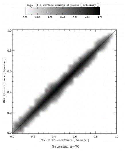
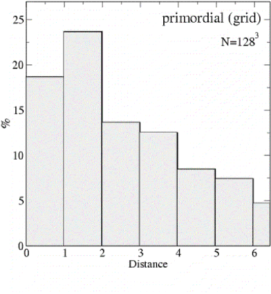
Figure 1: Performances of MAK reconstruction. left panel: Scatter plot of the MAK-reconstructed initial coordinates of a particle versus its initial, post-Zel’dovich coordinate for the $128^{3}$ particles ($S_{0}$ sample) in the Gaussian simulation. We use a “quasi-periodic projection” (QP) coordinate $\tilde{q}=(q_{1}+q_{2}\sqrt{2}+q_{3}\sqrt{3})/(1+\sqrt{2}+\sqrt{3})$, with $q_{1}$, etc… $\in[0,1]$ where 1 corresponds to the box size. These QP coordinates guarantee a 1-to-1 correspondence between the $\tilde{q}$-values and the points on a regular grid. To clearly show where the majority of particles reside on the diagram, we show the decimal logarithm of 1 plus the local density of points (the resolution is 1/256 in QP coordinate, and the Lagrangian mesh spacing is 1/128). Note that most of the particles lie almost perfectly on the diagonal already illustrating the success of MAK. right panel: Histogram of the distribution of the distances, expressed in units of mesh size, between the true Lagrangian, discrete, positions of each particle on the uniform grid and the position assigned to it by the MAK reconstruction. The first bin corresponds to what we call ”ideal” reconstruction, as shown in Table 1. If one adds up the percentages obtained in the first and the second bin, one should obtain a good estimate of the percentage of ”ideally” reconstructed positions for the sparse sample $S_{1}$, as is the case (see Table 1).

4 Efficiency of MAK as a nonlinear reconstructor

This section focuses on the Gaussian model. Firstly, we present detailed comparisons between the MAK-reconstructed displacement field with the non-linear displacement field (here after SIM NL) which it is designed to recover. Secondly, we compare the reconstructed and simulated nonlinear “density fields” that will be given by minus the divergence of the displacement field. We denote the latter by ${\bf v}$ and for this reason on occasions we refer to it as the “velocity field”. In both cases, comparisons with the Zel’dovich, initial conditions fields (hereafter SIM IC) are also given. Thirdly, we compare the present velocities found by MAK to the true peculiar velocities given by the simulation: the agreement on large scales is a notable achievement of our reconstruction method. In the last paragraph, we discuss potential resolution issues.

Except for Section 4.3 which concerns the present peculiar velocity field, the analyses are performed on the displacement field which is a Lagrangian quantity, always estimated as a function of Lagrangian coordinate, ${\bf q}$, on the primordial grid of initial unperturbed positions of the particles. In all cases, the measurements use the actual displacement between $z=\infty$ (the unperturbed grid) and $z=0$. For SIM IC, this requires a scaling of the linear displacement field using the Zel’dovich approximation.

Note furthermore that all the analyses in this section and in forthcoming ones are performed with additional top hat smoothing applied to the fields with spherical windows of various radii ($3\ h^{-1}$, $8\ h^{-1}$ Mpc, and sometimes $12\ h^{-1}$ Mpc). It is important to emphasize that top hat smoothing with a spherical window of radius $R$ is approximately equivalent to Gaussian smoothing with a window of radius $R/\sqrt{5}$. This should be kept in mind when comparing with previous works which usually use Gaussian smoothing (e.g. Monaco et al. 2000).

4.1 Comparison of the displacement fields

In the present and the next paragraph we analyse the $S_{1}$ sample of the Gaussian model to show that, as expected from the description of the algorithm in Section 3, MAK is an excellent tracer of the non-linear displacement field. We recall that the SIM NL displacement is simply measured in the simulation by joining a particle’s position on the Lagrangian grid to that particle’s position in the $z=0$ simulation output.

Fig. 2 compares, for SIM IC, MAK and SIM NL, the z-components of the displacement field projected along the z axis from a 20 $h^{-1}$ Mpc thick slice. The measurements have been performed using a nearest grid point (NGP) interpolation of the particles to a $64^{3}$ grid, followed by smoothing with a top-hat of radius 3 $h^{-1}$ Mpc . There is a very good agreement between the three panels of the figure. To have additional insight, Figure 3, displays $v_{\mathrm{z}}$ measured along a line. The two panels correspond to smoothing scales 3 $h^{-1}$ Mpc and 8 $h^{-1}$ Mpc . This figure highlights the subtle differences between the three panels of Fig. 2. In particular we see that the agreement between SIM NL and MAK is better than between SIM NL and SIM IC or between MAK and SIM IC. Note that even at mildly nonlinear scales, 3 $h^{-1}$ Mpc, the agreement between MAK and SIM NL is surprisingly good.

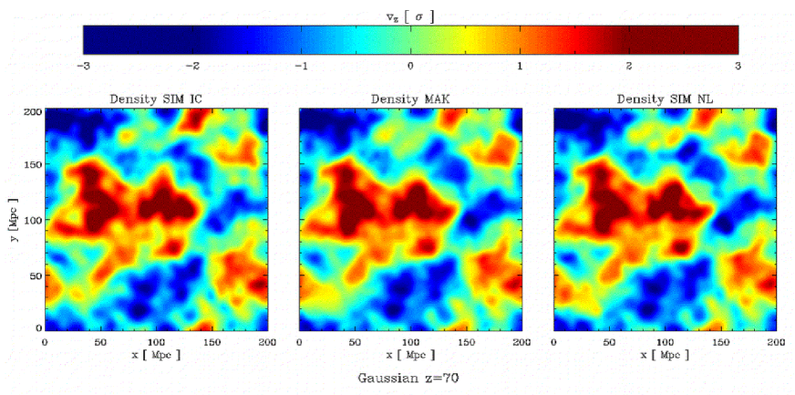
Figure 2: Projected $v_{\mathrm{z}}$ displacement field taken from a 20 $h^{-1}$ Mpc -thick slice normal to the z-direction, for the Gaussian model. The resolution before projection is $\sim$ 3 $h^{-1}$ Mpc in each direction. The left panel is the Zel’dovich initial conditions (SIM IC), the central panel is the MAK reconstruction and the right panel is the nonlinear displacement SIM NL. (Note that we will keep this tryptich structure and the corresponding SIM IC, MAK and SIM NL association for all remaining colour images.) The colour scale shown at the top is common to all plots and expressed in multiples of the rms of $v_{\mathrm{z}}$ of each field. The largest and broadest features repeat well in all three maps, but the MAK and SIM NL maps also match in detail.

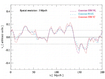
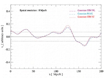
Figure 3: Profiles of the initial z-component of the displacement fields $v_{\mathrm{z}}$ in the Gaussian model, measured along a line parallel to the x-direction and located in the middle of the box. The resolution is 3 (resp. 8) $h^{-1}$ Mpc in the upper (resp. lower panel). The Zel’dovich SIM IC, MAK reconstruction and SIM NL profiles are shown with dotted, dashed and dash-dotted lines respectively. The horizontal dotted lines give $\pm\sigma$ of the SIM IC variations (the rms is measured from the profiles). Note how well MAK reproduces the SIM NL displacement field, even at 3 $h^{-1}$ Mpc resolution.

These results are confirmed by Fig. 4 which examines the PDFs of the $v_{\mathrm{z}}$ component of the displacement field, for SIM NL, MAK and SIM IC, at 3 $h^{-1}$ Mpc : the curves corresponding to MAK and SIM NL are nearly superimposed. They present a slight skewness which is due in the SIM NL case to non-Gaussianity brought by gravitational clustering. We already see that the latter feature is entirely captured by MAK.

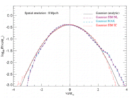
Figure 4: PDFs of the $v_{\mathrm{z}}$ displacement for the SIM IC (dotted line) and MAK reconstruction (dashed line) of the Gaussian model (rescaled to unit rms). The fields have been rescaled to unit rms.

So far we have compared single components of the displacement field: we now address the differences and/or similarities in amplitude and in direction between the three displacement fields as a function of the underlying over-density.

Figure 5 displays the measured distribution of the ratios $v_{\rm SIM\,IC}/v_{\rm MAK}$, $v_{\rm SIM\,NL}/v_{\rm MAK}$ and $v_{\rm SIM\,IC}/v_{\rm SIM\,NL}$ as a function of initial density estimated as minus the divergence of the initial displacement field. The upper and lower rows of panels correspond to a smoothing scale of 3 and 8 $h^{-1}$ Mpc respectively, prior to the calculation of their ratios. Again, the amplitudes of the MAK and SIM NL displacements agree well. The match is slightly less good for initially over-dense regions, as expected. Indeed, these regions might have experienced shell-crossing during dynamical evolution. Since SIM NL and MAK agree rather well, we notice similar discrepancy between SIM NL versus SIM IC and MAK versus SIM IC.

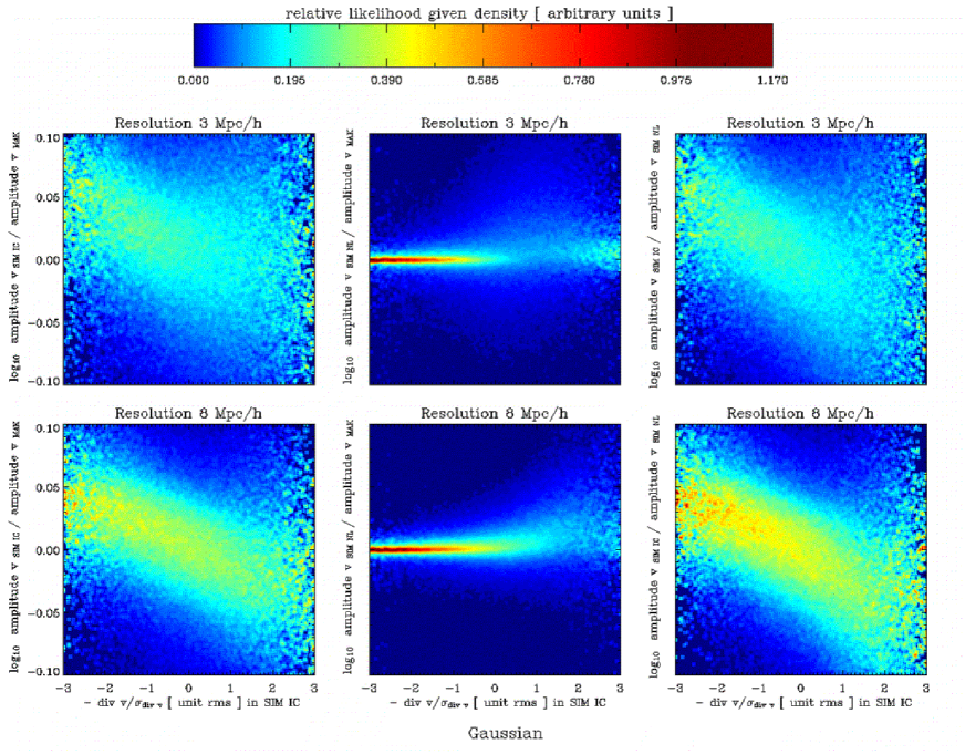
Figure 5: Left panels show the conditional PDF of the local ratio between the amplitudes of the Zel’dovich SIM IC and of the MAK-reconstructed displacements, as a function of the 3 $h^{-1}$ Mpc local over-density in the initial conditions SIM IC. The plot corresponds to the Gaussian model. The top (resp. bottom) row is for a 3 (resp. 8) $h^{-1}$ Mpc smoothing length. Middle panels: same as the left panels, but for the ratio between the amplitudes of the non-linear displacement field SIM NL and the reconstructed displacement field. Right panels: same as the left panels, but showing the ratio between the amplitudes of the Zel’dovich, SIM IC displacement field and the non-linear displacement field SIM NL.

Fig. 6 is the same as Fig. 5, but for the angle between the smoothed components of the displacement fields. The measured angle is always positive, but we made for clarity a reflection at the horizontal axis. To help understanding this figure one can assume for instance the SIM IC displacement direction to be chosen at random within a cone of angular size 10 (respectively 20) degrees centred on the MAK/SIM NL displacement direction. In this case, the observed distribution of angles would be bimodal and would peak at 6.7 (respectively 13.3) degrees.

In regions of low to average densities, the quality of the MAK reconstruction of the directions of the SIM NL displacement is striking. Above the mean density, the scatter starts to increase as expected again because these zones roughly correspond to virialized regions at $z=0$, where reconstruction is more difficult, but the bulk of the PDF remains within a $\pm$ 2 degrees offset. Note also that in the most strongly over-dense regions the displacement amplitudes are typically smaller than in regions of lower density, so that the consequences of significant errors in direction are not dramatic, simply because the magnitude of the displacement is small. On the other hand, comparing the MAK/SIM NL to SIM IC displacements, we find that the agreement is much less good, the most likely difference between the two directions being larger than $\sim 2.5$ degrees at the smoothing scales considered here.

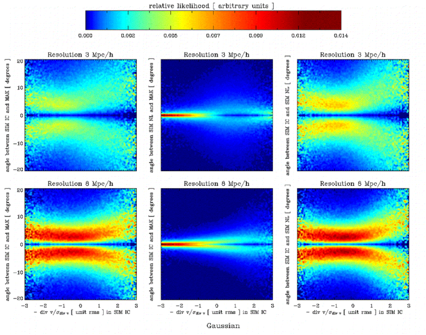
Figure 6: Same as Fig. 5 but for the angle [in degrees] between the displacement fields indicated by the vertical label of each plot, as a function of the over-density smoothed on a 3 $h^{-1}$ Mpc scale.

4.2 Comparison of the “density fields”

We estimate the density contrast, $\delta$, using the linear-regime relation $\delta({\bf x})\propto-\nabla_{q}\cdot{\bf v}$. For the SIM IC sample this is a fair estimate of the density field at this redshift. For the SIM NL and MAK samples, this basically gives an estimate of the primordial density by simple application of the Zel’dovich approximation.

In practice, to estimate $\nabla_{q}\cdot{\bf v}$, we first assign the displacement field of the particle set $S_{1}$ to a $64^{3}$ grid using nearest grid point interpolation (hereafter NGP) and then Fourier transform to take the gradient. As a result of taking the derivative, the $\nabla_{q}\cdot\bf v$ field is intrinsically more noisy than the displacement field. Fig. 7 is the pendant of Fig. 2 but for $\nabla_{q}\cdot\bf v$. It is supplemented with Fig. 8, which shows the 3- and 8 $h^{-1}$ Mpc smoothed divergence field computed along a line parallel to the $x$ direction cutting through the centre of the box.

The MAK density field clearly reproduces the SIM NL field very well at all values of $\nabla_{q}\cdot\bf v$. On the contrary, the MAK field only reproduces well the SIM IC field in regions of low to average densities. High-density ($\nu\sim 1.5-2$) patches are much more extended in MAK and in SIM NL than in SIM IC, and the $\nu\sim 2.5$ to 3 levels of the SIM IC field are barely reached by MAK or SIM NL.

This can be interpreted as follows. The fact that the simulated and the reconstructed displacement fields agree very well in the under-dense regions in all the cases is not surprising: indeed, the Zel’dovich mapping, hence SIM IC, is known, at least to some approximations, to work well in these regions (Sahni & Shandarin, 1996) and MAK reconstructs perfectly the Zel’dovich dynamics prior to the shell crossing. Therefore, in the under-dense regions, agreement among SIM IC, SIM NL and MAK is expected at least qualitatively. In detail, however, extra complications arise due to nonlinear dynamics which will be discussed below in more detail (see also Fig. 11).

In the over-dense regions, the interpretation of the results is more complex: the large patches with roughly constant density in SIM NL and MAK correspond to collapsed objects at $z=0$, as explicitly illustrated by Fig. 9 where we analyse a typical cluster at full resolution, i.e. extracted from the $S_{0}$ sample. Using Fig. 9 as a guideline, let us consider a Lagrangian region that will collapse to an object of negligible size, as illustrated by the upper left panel. It is trivial to realise that the displacement from the initial to the final stages is purely radial as shown in the left and right bottom panels for MAK and SIM NL respectively, and therefore that minus its divergence is equal to $3$, which is the upper bound expected for MAK reconstruction and for the simulation (more approximately in the latter case).

We thus see that the left and right bottom panels of Fig. 9 are extremely similar. They mostly differ in the boundary of the Lagrangian region occupied by the cluster: this means that the main difference between MAK and SIM NL relies on particles which have been assigned to the wrong collapsed objects. Particles that are not in the intersection of the two patches of the left and right bottom panels are clearly assigned wrongly by MAK and will give totally wrong displacement fields. We, however, notice that the boundaries of these ”peak patches” are nearly the same, which explains why MAK performs so well. At this point, it is important to notice that exact recovery of initial positions of particles belonging to the same collapsed object is not crucial and the quality of the reconstruction of the displacement field is only marginally affected if the positions of the particles ending up in the cluster are swapped by the MAK assignment. This demonstrates that there is no need to worry about the occasional low level of ”ideal” reconstruction presented in Table 1. Of course, the linear displacement field is not radial as shown in the upper right panel of Fig. 9, because it accounts for the details in the distribution of the initial fluctuations that are in the Lagrangian volume: in a hierarchical model such as CDM, smaller structures form first which then merge and create larger structures. In our picture, this would mean successive episodes of approximately locally radial displacements.

Clearly, Fig. 7 already emphasises the strengths and weaknesses of MAK: it seems to reconstruct the nonlinear displacement field and its divergence very well. However, the real goal is the recovery of the primordial density field: in this case, MAK performs qualitatively well in the under-dense regions but fails to do as well in the high-density regions due to the presence of collapsed structures, as explained above.

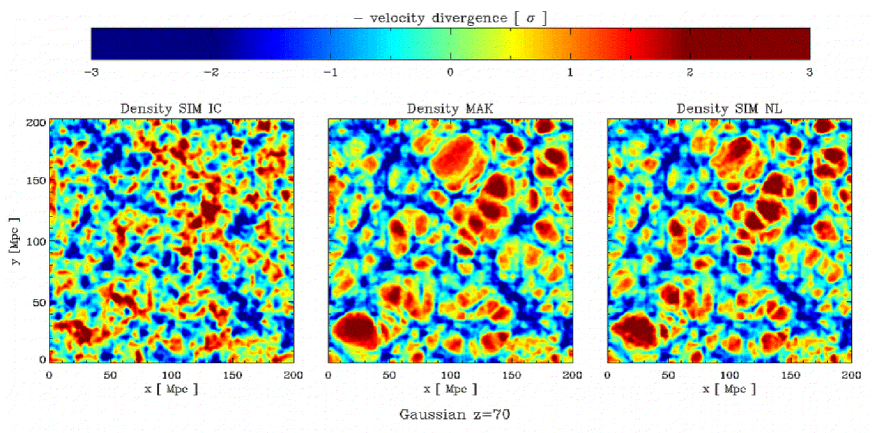
Figure 7: Same as Fig. 2 but for the projected negative divergence of the displacement field (proportional to the over-density in the linear regime). MAK reproduces very well the SIM NL field, at all densities. On the contrary, there are significant differences in regions of medium to high densities between the MAK and the SIM IC fields: $\nu=1.5$ to 2 regions are more patchy in MAK and SIM NL than in SIM IC, and the sharp, highest density peaks in SIM IC are not reproduced in the other two maps.

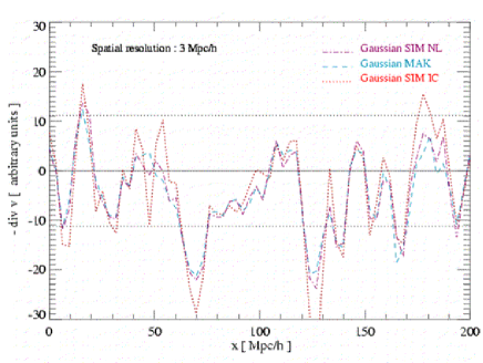
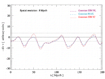
Figure 8: Same as Fig. 3, but for the divergence of the displacement fields. The resolution is 3 (resp. 8) $h^{-1}$ Mpc in the upper (resp. lower) panel. Again, MAK reproduces very well the SIM NL displacement field, even though the curves are more noisy than in Fig. 3, the consequence of taking the derivatives.

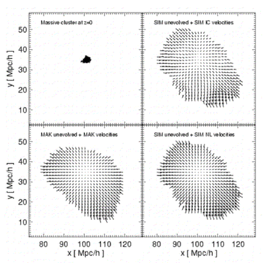
Figure 9: Upper left panel: z-projected simulated spatial distribution of particles of the third most massive cluster (with total mass $M_{\mathrm{tot}}=1.4\times 10^{15}\mbox{$h^{-1}$ $M_{\odot}$}$ and 4316 particles) of the Gaussian simulation at the present time. In this Figure we use the full resolution analysis, i.e., sample $S_{0}$. Upper right panel: z-projected Lagrangian region in the uniform grid for the particles ending in the cluster and the Zel’dovich SIM IC velocities. Lower left panel shows the MAK-reconstructed Lagrangian region and MAK-reconstructed displacement field. Lower right panel shows the true Lagrangian region (as in the top right panel) but with the SIM NL displacement field. We use arbitrary units but a common scale for all plots, so that the amplitudes can be compared. In the right top and right bottom panels we use the exact initial positions provided by the simulation and in the left bottom panel the Lagrangian region reconstructed by MAK.

To illustrate these results in a more quantitative way, Fig. 10 examines the PDF of the divergence of the displacement. The upper and lower panels of the figure correspond to the field smoothed here within a radius of $\sim 3$ $h^{-1}$ Mpc and $\sim 8$ $h^{-1}$ Mpc respectively. Again, the PDF of the MAK density field reproduces very well that of the SIM NL density field, including its positive skewness and its abrupt cutoff at large $\nu$ which corresponds to the present value of $-\nabla_{q}\cdot\bf v=3$ as discussed above.

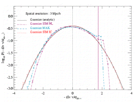
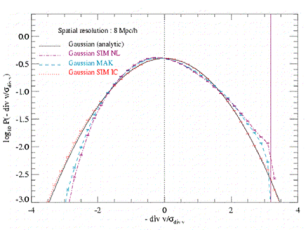
Figure 10: Same as Fig. 4 but for the divergence of the displacement field. The left and right figures correspond to $3$ $h^{-1}$ Mpc and $8$ $h^{-1}$ Mpc smoothing scales respectively. Both MAK and SIM NL which agree very well have a cutoff at large value of $\nu$ indicated by the vertical line (see text for further explanations).

Fig. 11 goes into deeper detail by examining the bivariate distributions: it represents scatter plots of the divergence of the displacement field for MAK versus SIM IC (left panels), MAK versus SIM NL (middle panels) and SIM NL versus SIM IC (right panels) computed for the fields smoothed at 3 and 12 $h^{-1}$ Mpc (upper and lower rows). The banana-shape observed in the right panels is due to nonlinear clustering and can be predicted from perturbation theory, similarly to what has previously been done for the divergence of the velocity field (Bernardeau, 1994b; Bernardeau et al., 1999). A calculation of $-\nabla_{q}\cdot{\bf v}$ relying on the spherical collapse model is given in Section  6 and displayed on the bottom right panel. If one neglects the cutoff expected for SIM NL at $-\nabla_{q}\cdot\bf v\sim 3$ the nonlinear gravitational effects increase the value of $-\nabla_{q}\cdot\bf v$ in the under-dense regions and increase it in the over-dense regions compared to the linear predictions. We notice here that the qualitative results stated previously about under-dense regions need to be quantified: even in the low density regime the recovery of the initial density field from the nonlinear displacement field can be nontrivial without further priors. In the middle panels, we see that MAK again agrees extremely well with SIM NL with a very small bias: the scatter around the diagonal is much smaller than in the right panels although we see, in the $3$ $h^{-1}$ Mpc smoothing case, an increase of the dispersion for positive values of $-\nabla_{q}\cdot{\bf v}$ and a slight bias at larger values of $-\nabla_{q}\cdot{\bf v}$. This comparison between SIM NL and MAK confirms fully the nontrivial nonlinear nature of MAK reconstruction. The left panels are very similar to the right panels, as expected.

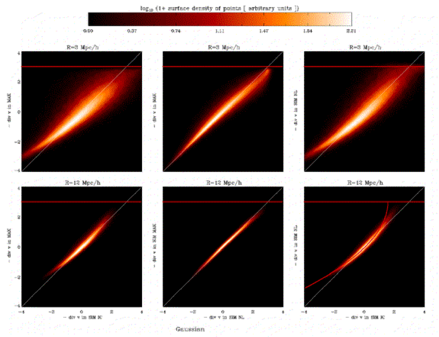
Figure 11: Scatter plots comparing in a point-by-point perspective (nodes of a regular grid) the density of the MAK field to the density of the SIM IC field (left panels), the MAK vs. SIM NL density fields (middle) and the SIM NL vs. SIM IC (right). The upper (resp. lower) panels are for a 3 (resp. 12) $h^{-1}$ Mpc smoothing length. We have used the negative divergence of the displacement as a proxy for the density. We recover the expected tight correlation between MAK and SIM NL and the absence of any significant bias. A horizontal line is displayed on each panel. It corresponds to the expected upper bound $-\nabla_{q}\cdot{\bf v}=3$ as discussed in the text. In the bottom right panel, the curve shows the result given by the spherical collapse approximation [see Eq. (11)]. The limitations of this model, discussed later in Section 6, justify the choice of $12\mbox{$h^{-1}$ Mpc}$ instead of $8\mbox{$h^{-1}$ Mpc}$ for the smoothing length.

4.3 Present-day peculiar velocity fields

An important and direct outcome of MAK reconstruction, the peculiar velocity field ${\bf v}_{\mathrm{MAK}}({\bf x})$, is a surprisingly good approximation to the present day true peculiar velocity field ${\bf v}_{\mathrm{pec}}({\bf x})$.

${\bf v}_{\mathrm{MAK}}({\bf x})$ for a given particle is obtained simply by scaling of the MAK displacement obtained previously at reconstructed particle’s position (node of the Lagrangian grid), and assigning the displacement to this particle’s position at $z=0$ following equations (7) and (8). It is unclear, except maybe at very large scales, that ${\bf v}_{\mathrm{MAK}}({\bf x})$ can approximate ${\bf v}_{\mathrm{pec}}({\bf x})$. Fig. 12 shows that this is indeed the case on scales of $8$ $h^{-1}$ Mpc. There, we show the $z=0$ $v_{\mathrm{x}}$-$v_{\mathrm{y}}$ velocity field extracted at $z=0$ from a 20 $h^{-1}$ Mpc -thick slice normal to the z-direction and cutting through the centre of the Gaussian simulation. (We use the $S_{1}$ sample in this Figure.) The left (resp. right) panel shows the ${\bf v}_{\mathrm{pec}}({\bf x})$ field given by the simulation (resp. ${\bf v}_{\mathrm{MAK}}({\bf x})$), smoothed with a top-hat kernel of radius 8 $h^{-1}$ Mpc. The underlying colour map gives the simulated dark matter density field smoothed on the same scale and then projected; it is the same for both panels. On these scales, we find excellent agreement between the simulated peculiar velocities and the reconstructed velocities.

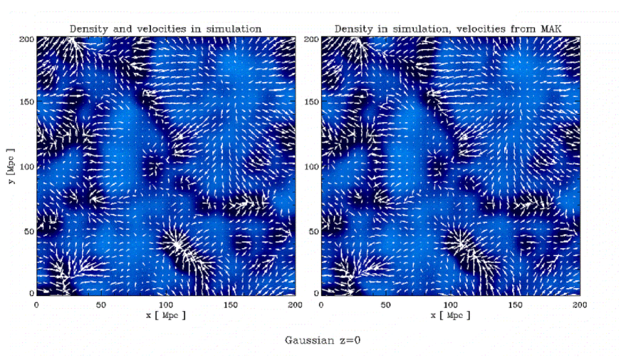
Figure 12: $z=0$ $v_{\mathrm{x}}$-$v_{\mathrm{y}}$ velocity field of a 20 $h^{-1}$ Mpc -thick slice normal to the z-direction cutting at a depth of $\sim 1/3$ of the simulation box in z through the Gaussian simulation; the left and right panels respectively correspond to the simulated (peculiar) velocity field and to the reconstructed velocity field. The 8 $h^{-1}$ Mpc smoothing scale guarantees that we are not affected by shell crossing. Underlying the velocity field we show in colour map the 3-dimensional density field at $z=0$ cut from the same z-slice and projected in z (it is the same density field in the left and right panels, and black is over-dense). There is quasi-perfect agreement between the two velocity fields.

On much smaller scales, Fig. 13 details the simulated and reconstructed present-day ($v_{\mathrm{x}}$,$v_{\mathrm{y}}$) components of ${\bf v}_{\mathrm{MAK}}({\bf x})$ and ${\bf v}_{\mathrm{pec}}({\bf x})$ for particles selected in a $4^{3}$ $h^{-1}$ Mpc region of the Gaussian simulation. (We use the $S_{0}$ sample here.) Although the agreement in the sparse/under-dense regions is still generally very good, differences arise between the simulated and the reconstructed particle velocities in regions of medium and higher densities.

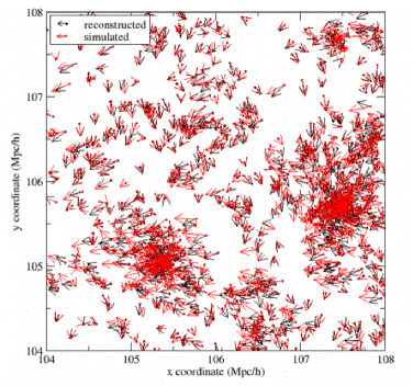
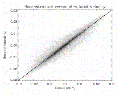
Figure 13: left panel: $z=0$ $v_{\mathrm{x}}$-$v_{\mathrm{y}}$ velocities of particles selected from a 4 $h^{-1}$ Mpc -side and 20$h^{-1}$ Mpc deep sub-volume taken from the Gaussian simulation. Simulated peculiar (resp. reconstructed) velocities are shown with the red (resp. black) arrows. There is fairly good agreement in the voids, but more noticeable differences in the outskirts of haloes. right panel: scatter plot of the reconstructed and simulation velocities at z=0 for the Gaussian sample of $64^{3}$, sample Gaussian $S_{1}$ of Table 1, demonstrates closely the goodness of the reconstructed velocity field. Axes are in box units (one unit is 200 $h^{-1}$ Mpc ).

A thorough comparison between MAK and other methods of proper-velocity evaluation (e.g. Yahil et al 1991 ; Valentine et al. 2000 and Shaya et al. 1995) remains to be done in future works where we plan to apply MAK to mock and large-scale redshift galaxy catalogues.

The very good agreement on scales of $\sim$ 8 $h^{-1}$ Mpc suggests a possible use of MAK to turn present-day redshift catalogues into real space catalogues, in an iterative process to deal with redshift space distortion. In applying MAK to real or mock galaxy catalogues, a quantitative error analysis is surely needed to access the goodness of MAK in evaluation of quantities such as cosmological parameters or mass to light ratio (some of these issues have been discussed in Mohayaee and Tully 2005 for the application of MAK to NearBy Galaxies (NBG) catalog).

4.4 Possible resolution issues

Our study of the resolution effects consisted of analysing the full resolution sample ($S_{0}$) and dense sample ($S_{2}$) [see Section 3.2 and Table 1] and of comparing the results to the sparse sample ($S_{1}$) used for most of the analyses up to now. We did not notice any significant differences between the full and sparse resolutions.

To illustrate our point, the top and bottom panels of Fig. 14 compare the PDFs of SIM IC, MAK and SIM NL density fields smoothed with a top-hat kernel of radius 3 and 8 $h^{-1}$ Mpc respectively using the full set $S_{0}$ of $128^{3}$ reconstructed particles. There are no significant differences with respect to the PDF of Fig. 10 computed for the set $S_{1}$. Note that this nice agreement between the sparse and full samplings is further supported by the right panel of Fig. 1 and the last column of Table 1: the ”ideally” reconstructed Lagrangian positions in $S_{1}$ are consistent with the fraction of the particles in $S_{0}$ that are reconstructed with accuracy better than two mesh sizes.

The dense sample, $S_{2}$, tests as well, to some extent, the importance of tidal and edge effects on the reconstruction. In practice, this can have important consequences for reconstructions of volume-limited (in the literal sense) catalogues which might not extend well above the scale of homogeneity. For the dense sample size considered here, $100$$h^{-1}$ Mpc , these effects seem to be negligible. For instance, the fraction of ”ideally” reconstructed particles is $17\%$ to be compared with the $18\%$ obtained for the full sample, $S_{0}$, reconstruction.

Note that we have performed these resolution tests as well for the $\chi^{2}$ model and the dense sample for the PVM and have obtained similar results.

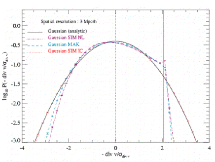
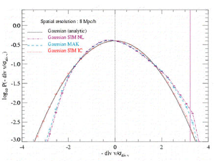
Figure 14: Same as Fig. 10 but for the full set $S_{0}$ of $128^{3}$ particles rather than its sparse sample, $S_{1}$.

5 Reconstructing non-Gaussian density fields

In this section, we examine different non-Gaussian initial conditions and verify if the results obtained previously for the Gaussian case still hold. We shall see that this is indeed the case, namely that the displacement fields reconstructed by MAK match extremely well their true nonlinear counterparts given by the simulations.

However, the real goal here is to study the properties of the initial density field or in other words the divergence of the initial displacement field which differs from the total final field, that is best reconstructed by MAK: the nonlinear contribution due to gravitational collapse should be subtracted from the reconstructed displacement field to allow tests for primordial non-Gaussianity. This will be confirmed by the subsequent analyses which will demonstrate that a “simple” use of MAK reconstruction is insufficient for recovery of a small level of non-Gaussianity. By “simple” we mean the extrapolation of the nonlinear displacement field to early epochs using the Zel’dovich approximation to infer the initial density field.

To carry out our analyses and reach these conclusions, we have explored the large spectrum of non-Gaussian models, detailed in Section 2:

1. The $\chi^{2}$ model, examined in Sec. 5.1, which is strongly non-Gaussian but with the same topological properties as its Gaussian seed;

2. The primordial voids model (PVM), studied in Sec. 5.2, which is strongly non-Gaussian and initially inhomogeneous;

3. The weakly non-Gaussian Quadratic ($Q$) models, discussed in Sec. 5.3.

5.1 $\chi^{2}$ model

In Fig. 15 we examine $-\nabla\cdot\bf v$ in a 10 $h^{-1}$ Mpc thick slice, similarly as in Fig. 7, while Fig. 16 compares the PDF of $-\nabla\cdot{\bf v}$ for SIM IC, MAK and SIM NL. The measurements are performed using a top-hat smoothing length of 8 $h^{-1}$ Mpc. The PDFs of MAK and SIM NL agree perfectly, which is consistent with the visual inspection of Fig. 15. They differ only slightly from SIM IC PDF. This might be surprising at first sight, because visually SIM NL and MAK look rather different from SIM IC, at least for large values of $-\nabla\cdot{\bf v}$. As explained in length in our study of the Gaussian model, this difference is mainly due to the presence of collapsed objects which induce an abrupt cut-off in the tail of the PDF for large values of $-\nabla\cdot{\bf v}$ (This cut-off lies outside the plot range in Fig. 16). However, a more careful inspection of Fig. 15 shows a much better agreement in regions of lower density, which explains the very good match between all of the three PDFs.

Except for the abrupt cut-off, the small difference as compared to the Gaussian case between the MAK/SIM NL PDF and SIM IC is due to two factors. First, the contribution from initial non-Gaussianity is strong enough to completely dominate over the contribution from gravity. Second, in this model the effect of gravitational clustering is less intense than in the Gaussian model because of the lower value of $\sigma_{8}$. A noticeable consequence of this lower normalisation is that there are less shell crossings and therefore the fraction of ”ideally” reconstructed particles is much higher than for the Gaussian model (see last column of Table 1).

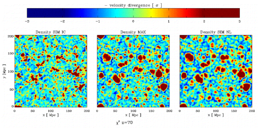
Figure 15: Same as lower panel of Fig. 7, but for the $\chi^{2}$ model.

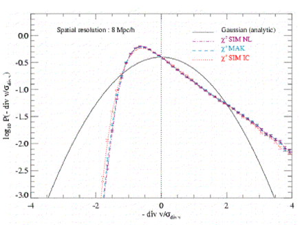
Figure 16: Same as Fig. 10 but for the $\chi^{2}$ model.

5.2 PVM model

In Fig. 17 we examine $-\nabla\cdot{\bf v}$, in a 10 $h^{-1}$ Mpc thick slice, similarly as in Fig. 7, while Fig. 18 compares the PDF of $-\nabla\cdot{\bf v}$ for SIM IC, MAK and SIM NL. The measurements are performed with a top-hat smoothing length of 8 $h^{-1}$ Mpc .

Recall that for PVM, initial conditions are strongly inhomogeneous at very high redshifts. As a result, it is in principle meaningless to use MAK reconstruction. However, at some point, the initial conditions had to be almost homogeneous, prior to the seeding of the primordial voids. Hence, we can still assume that we are starting from Lagrangian positions setup on a homogeneous grid. In our case, this homogeneous grid is the one where particles are located prior to the Zel’dovich displacement and void creation as explained in Section 2.3. With this in mind, a fair comparison between the middle and right panel of Fig. 17 can be made and again the visual agreement between MAK and SIM NL is excellent. Expectedly, due to the early strong nonlinearities induced by voids creation and subsequent shell crossings, the fraction of “ideally” reconstructed particles is rather low (28%, see Table 1).

From the previous arguments, comparing MAK/SIM NL to SIM IC has to be done with care. Clearly the strong “density contrasts” observed around voids in the left panel are expected to be smeared out in the middle and right panels. Keeping this in mind, we notice that there is a global large scale qualitative agreement between the three panels of Fig. 17, including the positions and extensions of the under-dense regions, although the amplitudes of the fluctuations are different. This means that our nonlinear displacements fields have kept at least some informations on the non-Gaussian nature of initial conditions even if the middle and right panels differ significantly from the left one.

The results of the previous discussion are nicely illustrated by Fig. 18 that we can now comment on in detail. The bell-shaped part of the SIM IC PDF corresponds to the initial Gaussian field generated prior to the seedings of the voids. The strong over-dense and under-dense regions appearing during the creation of the voids increase the variance of the density field by adding tails to the PDF both in the high and the low parts. This explains why the bell-shape of the SIM IC PDF on Fig. 18 is in fact narrower than a pure Gaussian with the same variance, given the choice of representation, in units of $-\nabla_{q}\cdot{\bf v}/\sigma$. Note that this additional contribution to the variance is, at least in the linear regime, a pure transient, as discussed furthermore at the end of Section 6. If one neglects additional non-Gaussianity brought about by gravitational instability, one thus expects that the bell-shaped part of the PDF converges to the pure Gaussian at late times, as one can indeed observe in Fig. 18.

The MAK and SIM NL PDFs agree with each other very well as expected. In the positive $-\nabla_{q}\cdot{\bf v}$ part, nonlinear gravitational clustering and subsequent shell crossings destroy information related to the strong over-dense spheres around the voids. As a result, in this regime the shape of the PDF is qualitatively very similar to what would be obtained from the Gaussian case. However, as noticed while examining Fig. 17, the informations on the primordial voids is still present in the tail for the low values of $-\nabla_{q}\cdot{\bf v}$. Clearly, despite the fact that SIM NL/MAK PDFs differ enormously from SIM IC PDF, they have still preserved a detectable signature of primordial non-Gaussianity.

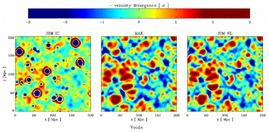
Figure 17: Same as Fig. 15, but for the PVM model. Again, the agreement between the MAK and SIM NL fields is very good.

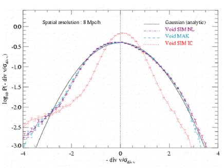
Figure 18: Same as Fig. 16 but for the PVM model.

5.3 Quadratic models

Fig. 19 shows the PDF of $-\bf{\nabla\cdot v}$ for the SIM IC, MAK and SIM NL, with a top-hat smoothing of 8 $h^{-1}$ Mpc for the series of quadratic models $Q$ (recall that these are models with very small non-Gaussianity). These models evolve to very similar nonlinear stages since they are all weakly non-Gaussian: gravity dominates significantly over initial non-Gaussianity suggesting that it will be nontrivial to recover the latter. Once again, the reconstructed nonlinear displacement field matches the simulated one for all of these models. As expected, the fraction of “ideally” reconstructed particles is similar to that in the Gaussian model ($41-43\%$ versus $37\%$, see last column of Table 1).

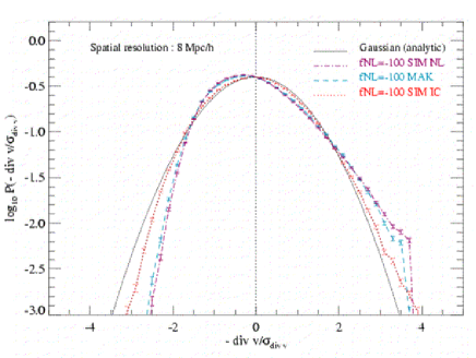
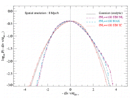
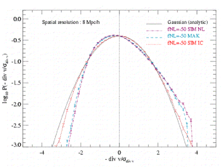
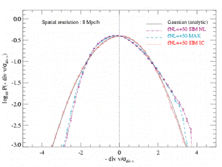
Figure 19: Same as Fig. 10, but for the series of quadratic models. $Q_{-100}$, $Q_{+100}$, $Q_{-50}$, $Q_{+50}$ respectively correspond to the upper left, upper right, lower left and lower right panels.

6 Separation of the initial and gravitational-induced non-Gaussianities: the spherical collapse model

We see that MAK reconstructs the nonlinear displacement field with a tremendous accuracy. The problem is that, in order to constrain the primordial non-Gaussianity, it is essential to recover the initial density contrast, i.e. the divergence of the linear displacement field. To achieve this goal it is necessary to model the effect of gravitational instability on the displacement field. Several approaches might be chosen:

1. Semi-analytic field reconstruction method in an iterative way. The method would inspire closely from the ideas developped in the building of ZTRACE reconstruction (Monaco & Efstathiou 1999), i.e. would be comparable to Peak-Patch (Bond & Myers, 1996) or Pinocchio (Monaco, Theuns & Taffoni, 2002), but in a reverse way. More explicitely, the idea is to use a realistic approximation of the dynamics depending in a unique way on the initial displacement field and the goal is to reconstruct the latter in an iterative manner. For instance, one can use Lagrangian perturbation theory up to some order, the latter being determined by the level of non-Gaussianity one aims to probe, e.g. the skewness (second order needed) or the skewness and the kurtosis (third order needed) of the initial distribution function. The subtlety of this approach is that one needs to truncate the sought-after initial fluctuations at some scale in order to deal appropriately with shell crossings in over-dense regions. The corresponding smoothing scale depends on location, according to the mass scale of the collapsed object formed at present time.

   If one uses Lagrangian perturbation theory, the nonlinear displacement field is indeed, for the growing mode, entirely determined as a function of the initial one, even if one has to take into account the adaptive smoothing of initial conditions needed for dealing with collapsed regions, as has just been explained. In this approach, the goal would then be to solve an implicit equation on the initial displacement field by equating the subsequent theoretical nonlinear displacement field with the reconstructed one by MAK. To solve this implicit equation, the most obvious approach would rely on an iterative method, which is unfortunately not guaranteed to converge.

2. Statistical method relying on loop perturbation theory. A less elegant, but simpler and still powerful method consists of working directly on the PDF of the divergence of the reconstructed displacement field to infer the PDF of the initial one. Again, some modelling of the dynamics is needed, to infer the mapping between the former and the latter. The best way to achieve that relies on perturbation theory and its one-loop (or higher order) corrections (e.g., Scoccimarro & Frieman, 1996). The advantage of this approach is that it allows one to probe scales which are close to the nonlinear regime. Since MAK reconstruction is very good, even at mildly nonlinear scales, this method would be optimal, but still quite involved from the analytic point of view.

3. Statistical method relying on the top-hat spherical model. To simplify furthermore the approach, with still in mind the goal of remapping of the probability distribution, one can use the top-hat spherical model (e.g., Fosalba & Gaztanaga, 1998a, b). This approximation has been demonstrated to work very well, both from the theoretical (Bernardeau, 1992, 1994a, 1994b; Gaztanaga & Fosalba, 1998; Fosalba & Gaztanaga, 1998a, b) and the numerical points of view (Fosalba & Gaztanaga, 1998a, b). However, it works only in the regime where fluctuations of the considered field (here the divergence of the displacement) are very small. Indeed, this model presents wrong loop corrections, but has the considerable advantage of relying on a very simple formalism.

It would be beyond the scope of this paper to try to apply approaches (i) and (ii) to our data, because they are both rather involved, from the numerical and analytical points of view. Instead, we concentrate on the spherical top-hat model, to demonstrate that it is possible to estimate the level of non-Gaussianity of the initial displacement field from the MAK-reconstructed one.

Under the top-hat spherical approximation, the divergence of the displacement field can be expressed as a function of the density contrast as follows:

$$\psi\equiv\nabla_{q}{\bf v}=3\left[(1+\delta)^{-1/3}-1\right].$$ (9)

We now relate $\psi$ to the initial linear density contrast, $\psi_{L}=-\delta_{L}$. In the spherical top-hat framework, the approximation

$$1+\delta\simeq\left(1-\frac{2}{3}\delta_{L}\right)^{-3/2}.$$ (10)

relates $\delta$ to $\delta_{L}$ (Bernardeau, 1994b). In the above equation, the time dependence of the growing mode extrapolated to present time has been included in $\delta_{L}$. This approximation turns out to be excellent, independently of the value of the cosmological parameters (Bernardeau, 1994b).

We thus obtain

$$\psi=3\left[\left(1+\frac{2}{3}\psi_{L}\right)^{1/2}-1\right].$$ (11)

In the spherical approximation framework, this gives us, in Lagrangian space, the transformation from the initial divergence of the displacement field to the final one. This formula is unchanged if top-hat smoothing is applied to the fields, here $\psi_{L}$ and $\psi$, under consideration (Bernardeau, 1994a).

Inverting Eq. (11), we obtain the simple relation

$$\psi_{L}=\frac{3}{2}\left[\left(1+\frac{\psi}{3}\right)^{2}-1\right].$$ (12)

The spherical collapse approximation has already been used to explicitly calculate the PDF in a local Lagrangian formalism (Protogeros & Scherrer 1997; Protogeros et al. 1997). The above equation gives us the change of variable to obtain the PDF of the initial divergence of the displacement field as a function of the non-linear, reconstructed one, by simply using

$$P(\psi_{L})d\psi_{L}=P(\psi)d\psi.$$ (13)

Note that the relation between $\psi$ and $\psi_{L}$ [Eq. (11)] imposes an upper bound on the possible values of $\psi_{L}$, $\psi_{L}\geq-3/2$, which in turns implies that $\psi\geq-3$, as already discussed extensively in Section 4.2. This also shows the limits of the spherical collapse approximation: it is expected to fail for collapsed objects, i.e. when $\psi$ approaches the bound $\psi=-3$, as illustrated by Fig. 11. There is in fact certainly a way to fix this by using other approximations in the highly nonlinear regime that we do not explore here (e.g. using the so called “halo model” for instance discussed in Scoccimarro et al. 2001).

Here we test the spherical collapse model approximation applied to the divergence of the MAK-reconstructed displacement field at a scale of $12\mbox{$h^{-1}$ Mpc}$, where we know that one-loop corrections are expected to be negligible and thus where the spherical collapse model should perform well, even in the non-Gaussian case, as argued by Fosalba & Gaztanaga (1998b).

We first examine in Fig. 20 the Gaussian, $\chi^{2}$ and $Q$ models. We shall pay attention to the special case of the PVM model at the end of this section. The success of the spherical model is unquestionable. Except in the tails (especially the right-handed one, as argued above), the shape of the initial PDF is recovered to very good accuracy. As discussed extensively in the caption of Fig. 20, even subtle features such as those observed in the $Q$ models are reproduced, lending credence to the fact that it seems possible to detect even small levels of primordial non-Gaussianity, at least with MAK reconstruction. Of course, this assertion does not take into account the instrumental and observational effects as shall be discussed later in the conclusion. Furthermore, our approach here is rather phenomenological, since we do not present a serious treatment of the statistical significance of the comparison.

We now turn to the PVM model. This model deserves a special treatment because the initial velocity field is not set up according to the Zel’dovich approximation, as explained in detail in Section 2.3. As a consequence, there are transients even for the variance of the displacement field: in the linear regime, the expanding voids are in fact pure transients, but they induce strong density contrasts that increase the variance of the fluctuations, thus the variance of the divergence of the displacement field. A consequence is that standard linear theory, with only the growing mode, does not apply. For instance, the value of $\sigma$ (where $\sigma^{2}$ is the variance of the field) at $12\mbox{$h^{-1}$ Mpc}$ measured in the initial $-\nabla\cdot{\bf v}$ scaled to present time is $0.94$, larger than the measured one from the nonlinear displacement field, 0.68. The spherical collapse model captures only the growing modes: they are determined by the initial Gaussian field prior to the void seeding. This one had a value of $\sigma$ of $0.71$, hence of the same order as the present one, as expected. In Fig. 21, we thus assumed for the comparison between true initial $-\nabla\cdot{\bf v}$ PDF and predicted one a value of $\sigma$ of $0.71$ for the latter. In practice, note that the test for non-Gaussianity does not need the precise knowledge of this initial $\sigma$: only the shape of the PDF matters, and has to be compared with the best fitting Gaussian in a trustworthy range.

Here the match between the predicted and the initial PDF is not so good anymore, although some non-Gaussian features seem to be captured, namely the right hand excess compared to the Gaussian case, but this might as well be a mere coincidence. The problem here is that the arguments in favour of the spherical top-hat model (e.g., Fosalba & Gaztanaga, 1998a, b) might not apply to the PVM model and its very strong transient nature, despite the fact that the voids are chosen here to be perfectly spherical. The validity of Eq. (11) and especially of the assertion that smoothing does not affect this equation is certainly questionable for the PVM model.

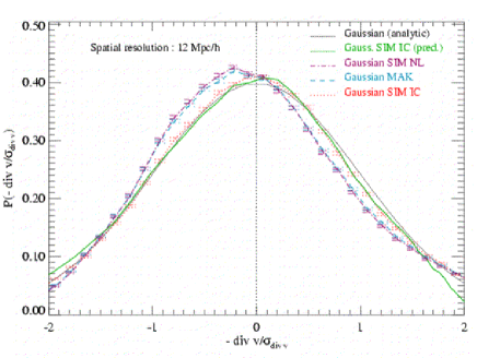
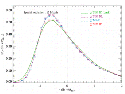
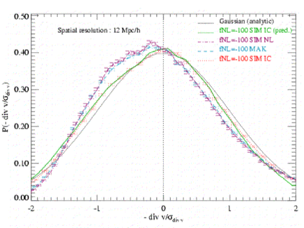
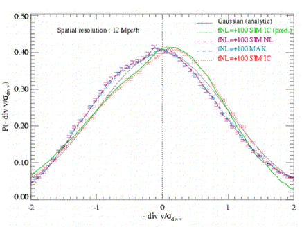
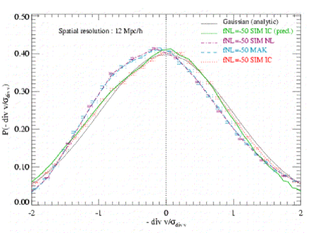
Figure 20: Comparison between the PDF of the true initial $-\nabla\cdot{\bf v}$ (SIM IC, dots) to the one inferred from the reconstructed displacement field using the top-hat spherical collapse approximation (SIM IC, predicted, thick solid curve), after a smoothing with a top-hat window of radius $12\mbox{$h^{-1}$ Mpc.}$ The choice of $12\mbox{$h^{-1}$ Mpc}$ instead of $8\mbox{$h^{-1}$ Mpc}$ is justified by the plots of Fig. 11. There are additional curves as detailed in the panels: the PDFs of $-\nabla_{q}\cdot{\bf v}$ for the nonlinear displacement fields, measured in the simulation (SIM NL, dot dashes) and reconstructed (MAK, dashes), and finally the pure Gaussian prediction (Gaussian, analytic, thin solid curve, not present on the upper right panel). Each panel corresponds to a given model as indicated on the figures. The important curves to examine on each panel are the dotted ones (initial PDF) and the thick solid ones (predicted initial PDF from the MAK nonlinear PDF), while keeping the Gaussian limit in mind: they should in principle superpose if the combination MAK+spherical collapse model works. This is indeed the case in all panels, except in the tails, especially the right-hand side one, but only for rather large values of $|-\nabla_{q}\cdot{\bf v}/\sigma_{\nabla\cdot{\bf v}}|\sim 2$. Indeed, in this regime, especially for positive values of $-\nabla_{q}\cdot{\bf v}$, the spherical collapse model is known to have limitations (e.g., Bernardeau, 1994b). Except for this, the agreement between the prediction and the measurement is excellent. It is in fact so good, that for the $Q$ models, the weakly non-Gaussian features are recovered, if one examines the upper part of the curves displayed in the four lower panels. The curves displayed on each are however slightly irregular, because the scale considered here is a significant fraction of the box size and the measured PDFs are thus expected to be contaminated by finite volume effects. This explains for instance the fact that in the Gaussian case, the dotted curve does not exactly superposed to the thin solid curve, i.e. the pure Gaussian prediction. Note that even this small deviation is reproduced by the MAK+top-hat prediction, at least for the right-hand part of the bell-shaped curves.

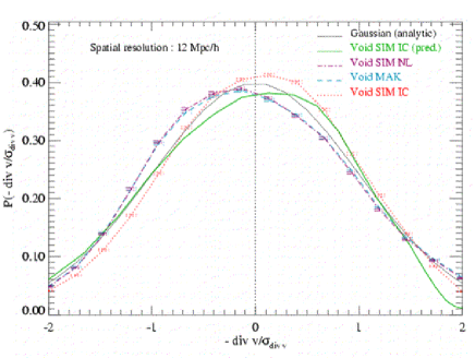
Figure 21: Same as in Fig. 20 but for the Void model.

7 Discussion

In this work, we have tested the Monge-Ampère-Kantorovich (MAK) reconstruction against $N$-body simulations. We have examined the standard $\Lambda$CDM model and 6 additional models with non-Gaussian initial conditions: a $\chi^{2}$ model where the initial density field is the square of a Gaussian, a model with primordial voids, and four mildly non-Gaussian models where the primordial gravitational potentials includes a small, quadratic correction.

The main results of this paper are as follows:

• In its essence, MAK is supposed to reconstruct the nonlinear displacement field between initial and final positions. The analyses of this paper show that it achieves this with an unprecedentedly high degree of accuracy, at least at scales larger than the size of rich clusters, i.e., scales above a few Mpc. In particular, it captures in a nontrivial way the nonlinear contribution from gravitational instability, well beyond the Zel’dovich approximation.

• From the MAK-reconstructed nonlinear displacement field, one can infer the present velocity field, using the Zel’dovich approximation. Again, our $N$-body simulation analyses demonstrate the success of MAK in fulfilling this goal.

• The displacement field provided by MAK can be used as well to constrain the statistical nature of the primordial density field. But, since MAK encodes nonlinearities due to gravitational clustering, it is difficult to disentangle these dynamical contributions from possible initial non-Gaussianities. However, as illustrated here in a simple way with the spherical collapse model, we show that it is possible to truly recover the statistical properties of the primordial, linear density field using additional modeling of the dynamics. Furthermore, we envisage possible improvements to be made by elaboration of MAK to a more sophisticated modeling of the dynamics combined with adaptive smoothing of the initial fluctuations [similarly as in ZTRACE (Monaco & Efstathiou 1999)].

The results presented in this paper are obtained in the “idealized” framework of $N$-body simulations. Extra complications arise in reconstruction from real galaxy catalogues (for application of MAK to real galaxy catalogues see Mohayaee & Tully 2004, 2005). Here, we discuss redshift space distortion, edge-effects, biasing and catalog incompleteness, which are the most relevant issues for MAK reconstruction:

1. Redshift space distortion: MAK has already been directly applied to redshift catalogues by modifying the cost function (6) using once again the Zel’dovich approximation (for detail, see Mohayaee & Tully 2004). An alternative method would be to deduce real space positions from redshift space data, using MAK in an iterative way. Indeed, we have shown in paragraph 4.3 very good agreements between the present-day simulated peculiar velocities and the MAK-reconstructed ones already on $\sim$ 8 $h^{-1}$ Mpc scales.

2. Boundary effects: in this paper, we have partly addressed edge and tidal effects using the dense samples. We have noticed that these effects are small but the volume considered was large, a cube 100 $h^{-1}$ Mpc aside. Clearly, large scale tidal effects and wrong assignments near the edges of a catalog would be important if it had a small volume coverage or/and intricate boundaries.

3. Biasing: in a real galaxy catalog, there is the problem of biasing that is the relationship between the present total matter distribution and the present observed light distribution. For each observed galaxy of a given luminosity, $L$, one has to infer a given mass which for instance can be a simple function of $L$. In this way, one can transform a distribution of points with given luminosities to a distribution of points with given masses. A supplementary complication arises since MAK requires in essence all the points to have the same mass. To achieve this, one can break the galaxies into equal mass particles, place them at the position of the galaxy and perform MAK reconstruction. In the hierarchical clustering framework, galaxies are located in dark matter halos, that is in condensed objects. We know from the results of this paper that MAK reconstructs very well the nonlinear displacement field even for regions that have experienced shell-crossings. In the latter case, the only problem is the wrong assignment of the particles inside the collapsed objects, but this does not affect the reconstruction of the displacement field significantly, and hence the velocity field inferred from it using the Zel’dovich approximation. Therefore, provided that the right mass has been given to each galaxy and that the catalog is complete enough so that the underlying total mass distribution is well-traced, the reconstruction is expected to perform well (Mohayaee & Tully 2004, 2005). There is however a subtlety which has to be taken into account, during mass assignment to galaxies: a different treatment has to be performed for field galaxies which have their own halo and galaxies belonging to rich clusters. In the latter case, what matters is the mass of the halo of a cluster and not the mass of the “sub-halos” of each of its galaxies (Mohayaee & Tully 2005).

4. Luminosity segregation: the last issue to consider is catalog incompleteness. For instance, in a standard magnitude-limited catalog, there is a luminosity segregation effect which arises due to fewer and brighter objects with increasing distance from the observer. It is possible to compensate for it by assigning a larger mass to more distant galaxies (Mohayaee & Tully 2005): this means that two galaxies of the same luminosity but at different distances from the observer will be given different masses. With this procedure, the reconstruction is in principle expected to be as least biased as possible. However, clearly the signal-to-noise ratio would decrease with distance from the observer, and more subtlely, the expected strong dependence of galaxy clustering with luminosity might complicate the interpretation of the results: obviously, it is needed to have catalogs complete enough in the faint end of the luminosity function in order to treat appropriately the biasing issues discussed in previous point.

References

- Acquaviva et al. ( 2003) Acquaviva V., Bartolo N., Matarrese S., Riotto A., 2003, NPB, 667, 119
- Amara & Refregier (2004) Amara A., Refregier A., 2004, MNRAS, 351, 375
- Arnold (1978) Arnold V. I., 1978, Mathematical Methods of Classical Mechanics. Springer, Berlin
- Avelino et al. (1998) Avelino P. P., Shellard E. P. S., Wu J. H. P., Allen B., 1998, ApJ, 507, 101
- Bahcall et al. (2003) Bahcall N. A., Dong F., Bode P., Kim R., Annis J., McKay T. A., Hansen S., Gunn J., Ostriker J. P., et al. 2003, ApJ, 585, 182
- Bartolo et al. ( 2004) Bartolo N., Komatsu E., Matarrese S., Riotto A., 2004, PhR, 402, 103
- Benamou & Brenier (2000) Benamou J.-D., Brenier Y., 2000, Numer. Math., 84, 375
- Bernardeau (1992) Bernardeau F., 1992, ApJ, 390, L61
- Bernardeau (1994a) Bernardeau F., 1994, A&A, 291, 697
- Bernardeau (1994b) Bernardeau F., 1994, ApJ, 427, 51
- Bernardeau et al. (1999) Bernardeau F., Chodorowski M. J., Lokas E. L., Stompor R., Kudlicki A., 1999, MNRAS, 309, 543
- Bernardeau & Uzan (2002) Bernardeau F., Uzan J., 2002, PRD, 66, 103506
- Bertschinger (1985) Bertschinger E., 1985, ApJS, 58, 1
- Bertsekas (1998) Bertsekas D. P., 1998, Network Optimisation: Continuous and Discrete Models. Athena Scientific
- Bond & Myers (1996) Bond J. R., Myers S. T., 1996, ApJS, 103, 41
- Bouchet et al. (1992) Bouchet F. R., Juszkiewicz R., Colombi S., Pellat R., 1992, ApJL, 394, L5
- Brenier et al. (2003) Brenier Y., Frisch U., Hénon M., Loeper G., Matarrese S., Mohayaee R., Sobolevskiĭ A., 2003, MNRAS, 346, 501, (B of FMB)
- Bunn et al. (1995) Bunn E. F., Scott D., White M., 1995, ApJL, 441, L9
- Chiu et al. (1998) Chiu W. A., Ostriker J. P., Strauss M. A., 1998, ApJ, 494, 479
- Couchman et al. (1995) Couchman H. M. P., Thomas P., Pearce F., 1995, ApJ, 452, 797
- Croft & Gaztanaga (1997) Croft R. A., Gaztanaga E., 1997, MNRAS, 285, 793
- El-Ad & Piran (2000) El-Ad H., Piran T., 2000, MNRAS, 313, 553
- Feldman et al. (2001) Feldman H. A., Frieman J. A., Fry J. N., Scoccimarro R., 2001, Physical Review Letters, 86, 1434
- Fosalba & Gaztanaga (1998a) Fosalba P., Gaztanaga E., 1998a, MNRAS, 301, 503
- Fosalba & Gaztanaga (1998b) Fosalba P., Gaztanaga E., 1998b, MNRAS, 301, 535
- Frisch et al. (2002) Frisch U., Matarrese S., Mohayaee R., Sobolevskiĭ A., 2002, Nature, 417, 260, (F of FMB)
- Gaztanaga & Fosalba (1998) Gaztanaga E., Fosalba P., 1998, MNRAS, 301, 524
- Gramann (1993) Gramann M., 1993, ApJ, 449, 405
- Griffiths et al. (2003) Griffiths L. M., Kunz M., Silk J., 2003, MNRAS, 339, 680
- Hénon (1992) Hénon M., 1992, math.OC/0209047 on arXiv
- Hénon (1995) Hénon M., 1995, in Compte Rendu de l’Academie des Sciences Vol. 321. p. 741
- Hoyle & Vogeley (2004) Hoyle F., Vogeley M. S., 2004, ApJ, 607, 751
- Juszkiewicz et al. (1993) Juszkiewicz R., Bouchet F. R., Colombi S., 1993, ApJL, 412, L9
- Komatsu et al. (2003) Komatsu E., Kogut A., Nolta M. R., Bennett C. L., Halpern M., Hinshaw G., Jarosik N., Limon M., Meyer S. S., Page L., Spergel D. N., Tucker G. S., Verde L., Wollack E., Wright E. L., 2003, ApJS, 148, 119
- Koyama et al. (1999) Koyama K., Soda J., Taruya A., 1999, MNRAS, 310, 1111
- La & Steinhardt (1989) La D., Steinhardt P. J., 1989, PRL, 62, 376
- Linde & Mukhanov (1997) Linde A., Mukhanov V., 1997, PRD, 56, 535
- Maldacena (2003) Maldacena J., 2003, Journal of High Energy Physics, 5, 13
- Matarrese et al. (2000) Matarrese S., Verde L., Jimenez R., 2000, ApJ, 541, 10
- Mathis et al. (2004) Mathis H., Silk J., Griffiths L. M., Kunz M., 2004, MNRAS, 350, 287
- Mohayaee et al. (2003) Mohayaee R., Frisch U., Matarrese S., Sobolevskiĭ A., 2003, A&A, 406, 393, (M of FMB)
- Mohayaee & Tully (2004) Mohayaee R., Tully R. B., U. Frisch, 2004, Invited contribution to Colloquium Cosmology: facts and Problems, College de France, Paris 8-11, June 2004, Eds. J.V. Narlikar, J-.C. Pecker, astro-ph/0410063
- Mohayaee & Tully (2005) Mohayaee R., Tully R. B., 2005, The cosmological mean density and its local variations probed by peculiar velocities, astro-ph/0509313
- Monaco et al. (2000) Monaco P., Efstathiou G., Maddox S. J., Branchini E., Frenk C. S., McMahon R. G., Oliver S. J., Rowan-Robinson M., Saunders W., Sutherland W. J., Tadros H., White S. D. M., 2000, MNRAS, 318, 681
- Monaco & Efstathiou (1999) Monaco P., Efstathiou G., 1999, MNRAS, 308, 763
- Monaco, Theuns & Taffoni (2002) Monaco P., Theuns T., & Taffoni G., 2002, MNRAS, 331, 587
- (47) Moscardini L., Matarrese S., Lucchin F., Messina A., 1991, MNRAS, 248, 424
- Nusser & Branchini (2000) Nusser A., Branchini E., 2000, MNRAS, 313, 587
- Nusser et al. (1995) Nusser A., Dekel A., Yahil A., 1995, ApJ, 449, 439
- Occhionero & Amendola (1994) Occhionero F., Amendola L., 1994, PRD, 50, 4846
- Peacock et al. (2001) Peacock J. A., Cole S., Norberg P., Baugh C. M., Bland-Hawthorn J., Bridges T., Cannon R. D., Colless M., et al. 2001, Nature, 410, 169
- Peebles (1980) Peebles P. J. E., 1980, The large-scale structure of the universe. Princeton University Press
- Peebles (1983) Peebles P. J. E., 1983, ApJ, 274, 1
- Peebles (1987) Peebles P. J. E., 1987, ApJ, 317, 576
- Peebles (1989) Peebles P. J. E., 1989, ApJL, 344, L53
- Peebles (1999) Peebles P. J. E., 1999, ApJ, 510, 523
- Peebles (2001) Peebles P. J. E., 2001, ApJ, 557, 495
- Peiris et al. (2003) Peiris H. V., Komatsu E., Verde L., Spergel D. N., Bennett C. L., Halpern M., Hinshaw G., Jarosik N., Kogut A., Limon M., Meyer S. S., Page L., Tucker G. S., Wollack E., Wright E. L., 2003, ApJS, 148, 213
- Pen et al. (2003) Pen U., Zhang T., van Waerbeke L., Mellier Y., Zhang P., Dubinski J., 2003, ApJ, 592, 664
- Protogeros & Scherrer (1997) Protogeros Z. A. M., Scherrer R. J., 1997, MNRAS, 284, 425
- Protogeros et al. (1997) Protogeros Z. A. M., Melott A. L., Scherrer R. J., 1997, MNRAS, 290, 367
- Robinson & Baker (2000) Robinson J., Baker J. E., 2000, MNRAS, 311, 781
- Robinson et al. (2000) Robinson J., Gawiser E., Silk J., 2000, ApJ, 532, 1
- Sahni & Shandarin (1996) Sahni V., Shandarin S., 1996, MNRAS, 282, 641
- Scoccimarro & Frieman (1996) Scoccimarro R. & Frieman J., 1996, ApJS, 105, 37
- Scoccimarro et al. (2001) Scoccimarro R., Sheth R. K., Hui L., & Bhuvnesh J., 2001, ApJ, 546, 20
- Scoccimarro et al. (2004) Scoccimarro R., Sefusatti E., Zaldarriaga M., 2004, PRD, 69, 103513
- Shaya et al. (1995) Shaya E. J., Peebles P. J. E., Tully R. B., 1995, ApJ, 454, 15
- Spergel et al. (2003) Spergel D. N., Verde L., Peiris H. V., Komatsu E., Nolta M. R., Bennett C. L., Halpern M., Hinshaw G., Jarosik N., Kogut A., Limon M., Meyer S. S., Page L., Tucker G. S., Weiland J. L., Wollack E., Wright E. L., 2003, ApJS, 148, 175
- Springel et al. (2001) Springel V., Yoshida N., White S. D. M., 2001, New Astronomy, 6, 79
- Takada & Jain (2004) Takada M., Jain B., 2004, MNRAS, 348, 897
- Tegmark et al. (2004a) Tegmark M., Blanton M. R., Strauss M. A., Hoyle F., Schlegel D., Scoccimarro R., Vogeley M. S., Weinberg D. H., Zehavi I., Berlind A., Budavari T., Connolly A., 2004, ApJ, 606, 702
- Tegmark et al. (2004b) Tegmark M., Strauss M. A., Blanton M. R., Abazajian K., Dodelson S., Sandvik H., Wang X., Weinberg D. H., Zehavi I., Bahcall N. A., Hoyle F., Schlegel D., Scoccimarro R., Vogeley M. S., Berlind A., Budavari T., Connolly A., 2004, PRD, 69, 103501
- Valentine et al. (2000) Valentine H., Saunders W., Taylor A., 2000, MNRAS, 319, L13
- van Waerbeke et al. (2001) van Waerbeke L., Mellier Y., Radovich M., Bertin E., Dantel-Fort M., McCracken H. J., Le Fèvre O., Foucaud S., Cuillandre J.-C., Erben T., Jain B., Schneider P., Bernardeau F., Fort B., 2001, A&A, 374, 757
- Verde & Heavens (2001a) Verde L., Heavens A. F., 2001, ApJ, 553, 14
- Verde et al. (2001) Verde L., Jimenez R., Kamionkowski M., Matarrese. S., 2001, MNRAS, 325, 412
- Verde et al. (2000b) Verde L., Wang L., Heavens A. F., Kamionkowski M., 2000, MNRAS, 313, 141
- White (1999) White M., 1999, MNRAS, 310, 511
- Wright et al. (1994) Wright E. L., Smoot G. F., Kogut A., Hinshaw G., Tenorio L., Lineweaver C., Bennett C. L., Lubin P. M., 1994, ApJ, 420, 1
- Zel’dovich (1970) Zel’dovich Y. B., 1970, A&A, 5, 84