The discrepancy between solar abundances and helioseismology

Abstract

There have been recent downward revisions of the solar photospheric abundances of Oxygen and other heavy elements. These revised abundances along with OPAL opacities are not consistent with seismic constraints. In this work we show that the recently released OP opacity tables cannot resolve this discrepancy either. While the revision in opacities does not seem to resolve this conflict, an upward revision of Neon abundance in solar photosphere offers a possible solution to this problem.

1 Introduction

Recent analyses of spectroscopic data using modern three dimensional hydrodynamic atmospheric models have suggested that the solar abundance of Oxygen and other abundant elements needs to be revised downward (Allende Prieto, Lambert & Asplund 2001, 2002; Asplund et al. 2004a,b; Melendez 2004). Asplund et al. (2004a) claim that the Oxygen abundance should be reduced by a factor of about 1.48 from the earlier estimates of Grevesse & Sauval (1998). The abundances of C, N, Ne, Ar and other elements are also reduced (Asplund et al. 2004b). As a result, the ratio (by mass) of heavy element to hydrogen abundance, $Z/X$, reduces from 0.023 to 0.0165, which causes the heavy element abundance in the solar envelope to reduce from $Z=0.017$ to 0.0122. This will cause the opacity of solar material to decrease, in turn reducing the depth of the convection zone (henceforth CZ) in solar models. Bahcall & Pinsonneault (2004) have constructed a standard solar model using these revised abundances to find that the depth of the CZ is indeed reduced significantly making it inconsistent with seismically established value. Basu & Antia (2004) and Bahcall et al. (2004a, 2005) also attempted to study solar models with reduced abundances and found that opacities near the base of the convection zone needs to be increased by 10–20% to make them consistent with seismic data. Turck-Chièze et al. (2004) also find that solar models constructed using revised heavy element abundances are not consistent with seismic inferences. Subsequently, Asplund et al. (2004b) have revised the abundances of some elements still further. As a result, the discrepancy can be expected to be somewhat larger.

Since the discrepancy can be attributed to reduced opacities, there is a need to examine the opacity calculations. Recently, Seaton & Badnell (2004) and Badnell et al. (2004) have carried out independent opacity calculations under the OP project. Near the base of the solar CZ, they only find a 2% increase in opacity as compared to OPAL. This is not likely to resolve the discrepancy, but nevertheless, the effect needs to be studied in detail. Since two completely independent opacity calculations agree very well with each other, it is unlikely that any possible revision in opacity will be large enough to address the discrepancy caused by the downward revision of solar abundances. Nevertheless, additional independent tests of opacity calculations are desirable to ensure reliability of opacities which are crucial input to stellar model calculations.

In this work we also study the effect of varying abundances of many heavy elements separately to check which of them are effective in addressing the discrepancy. Such studies will help in identifying the elements which play a crucial role in the discrepancy in solar models. It turns out that the problem may be resolved if the Neon abundance is increased by about 0.6 dex, i.e., by a factor of 4. It may be noted that the Neon abundance in the photosphere cannot be determined spectroscopically and hence the uncertainties could be large.

2 The technique

Following Basu & Antia (2004) we construct solar envelope models with different heavy element abundances. All these models have the seismically estimated hydrogen abundance, $X$, of 0.739 (Basu & Antia 1995, 2004) and the depth of the convection zone of $0.2867R_{\odot}$ (Christensen-Dalsgaard et al. 1991; Basu & Antia 1997, 2004). As a result there are no free parameters in these models and the sound speed and density in these models can be compared with seismically inferred values to check for consistency. These models use the OPAL equation of state (EOS) (Rogers & Nayfonov 2002) and opacity tables from OPAL (Iglesias & Rogers 1996) or OP (Badnell et al. 2004). In all cases, the opacity has been calculated using the appropriate mixture of heavy elements, while the EOS has been calculated using a standard mixture for which the OPAL tables are available. In principle, the EOS tables also need to be modified in view of the change in mixture of heavy elements. That has not been done since the EOS is not particularly sensitive to the detailed breakup of heavy element abundance.

We construct solar envelope models using the heavy element abundances as given by Grevesse & Sauval (1998) (referred to as GS98) or Asplund et al. (2004b) (referred to as Asp04). Furthermore, to study the effect of abundances of individual heavy elements, we have constructed models where the abundances of C, N, O, Ne, Mg, Si, S and Fe are separately reduced as compared to their abundances in GS98. For each solar envelope model we compare the density profile in the lower part of the convection zone with that inferred through seismic inversions. In general, the two do not agree with each other and we need to modify the opacity near the base of the convection zone to get agreement. The opacity modification required to get the density to agree is a measure of consistency between seismic data, abundances and opacities.

3 Results

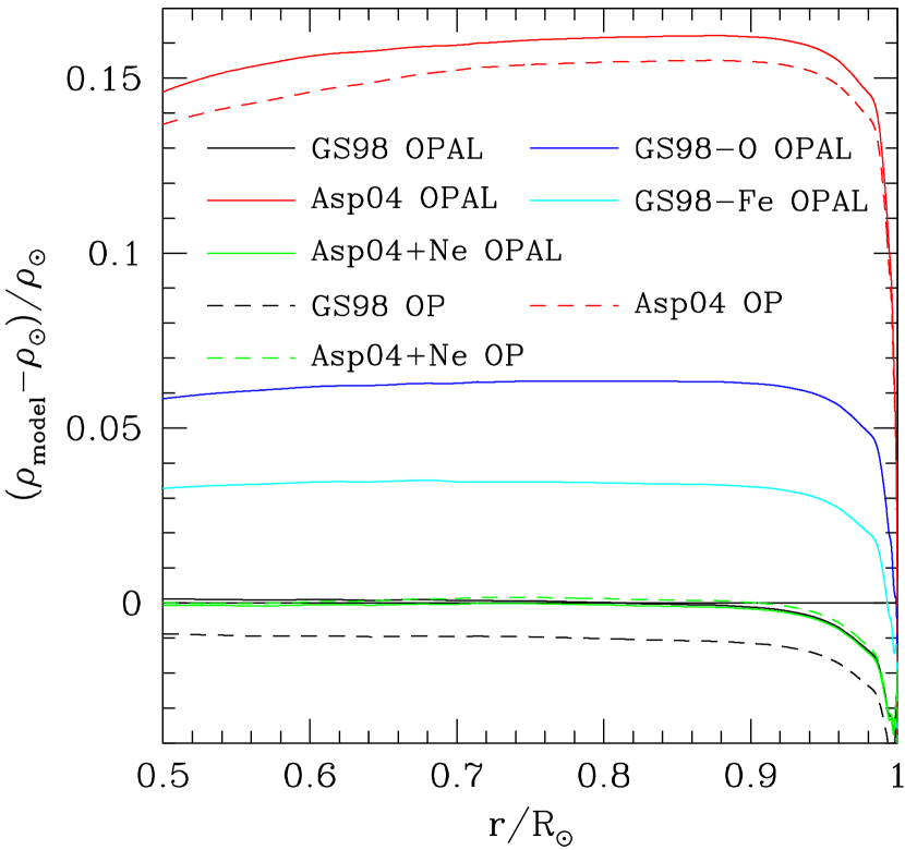
Figure 1: The relative difference in density between different solar envelope models and the Sun. The models are constructed using different heavy element mixtures and using either OPAL or OP opacity tables as marked in the figure. The model Asp04+Ne is with enhanced Ne abundance in Asp04 mixture, while GS98-O and GS98-Fe are with reduced O and Fe abundance respectively, in GS98 mixture. The curve for GS98 OPAL has merged with that for Asp04+Ne OPAL and hence is not clearly visible.

We compare the density profile in each solar envelope model with seismically inverted density and the results for some of the models are shown in Fig. 1. It is clear that the density profile in models constructed using the revised abundances is significantly different, from that of the Sun, the densities being higher than solar density. The estimated errors in the density inversion results in the lower CZ is about 1.5%, including systematic errors due to uncertainties in X, EOS etc. (Basu & Antia 2004). The difference in density is more than 15%, much larger than the errors. On the other hand, models with GS98 abundances have density profiles within error limits, thus these models are consistent with seismic constraints. For the Asp04 mixture the opacities need to be increased by $(27\pm 3)$% for OPAL models and $(25\pm 3)$% for OP models to get the density profile in agreement with seismic inversions. The OP and OPAL models for the same mixture are close to each other and the difference between them are consistent with known differences in opacity estimates.

It is clear from Fig. 1 that there is not much difference between models using OPAL and OP opacities. In order to quantify the differences in opacities, Fig. 2 shows the relative difference between the two opacities as a function of temperature in a solar model using Asp04 mixture. The differences are taken at the same density and temperature and reflect the differences in the actual opacity calculations. The differences are generally less than 2% in the radiative interior. Near the base of the CZ the difference is of order of 1%.

Since the two independent opacity calculations agree remarkably well with each other, it is unlikely that the discrepancy caused by reduced abundances can be due to uncertainties in opacities. To separate out the contribution of each element we construct a series of solar envelope models with the GS98 mixture, with the abundance of one element at a time reduced by the amount shown in the third column of Table 1. Two of these models (for reduction in O and Fe abundances) are also shown in Fig. 1. The results using OPAL opacity tables are summarized in Table 1, which lists the required opacity modification to restore the density profile to that inferred by inversions. It also lists the logarithmic derivative of the required opacity modification with respect to abundance of each element. It is clear that the derivative is significant for abundant elements like O, Ne, Fe. Thus the required opacity modification can be controlled by adjusting the abundance of some of these elements. And we see from Fig. 1, that the model with the increased Ne abundance is actually consistent with seismic results. If we believe that the abundance determination of O, Fe have improved significantly in recent times, then there may not be much uncertainty in their estimated abundance and we do not have much freedom to vary those abundances. The photospheric abundance of Ne however, may involve higher uncertainties since it can not be determined spectroscopically due to lack of suitable photospheric lines and has to be determined from coronal lines. This could also involve uncertainties due to possible fractionation in these layers, as the coronal Ne abundance may not reflect that in the photosphere. Thus we speculate that the effect of reduction in abundance of other elements like C, N, and O may be compensated by an increase in the Ne abundance. The required Ne abundance can be estimated by constructing models with different values of Ne abundance to estimate the required abundance to match the density profile. It turns out that we need an increase in Ne abundance by $0.63\pm 0.06$ dex when OP opacities are used, and by $0.67\pm 0.06$ dex when OPAL opacities are used. This corresponds to an increase in abundance by a factor of just over 4. It can be seen from Fig. 1 that the envelope models constructed using these abundances have the correct density profile. We can also estimate the required increase in Ne abundance from the partial derivative given in Table 1, but that gives a somewhat larger estimate, presumably because the derivative itself would increase when Ne abundance increases by a factor of 4.

Primary seismic inversions for sound speed and density are independent of opacities, but we need to use opacities in order to infer the temperature and hydrogen abundance profiles in the solar interior (Gough & Kosovichev 1988; Shibahashi & Takata 1996; Antia & Chitre 1998). We therefore check the differences in the inferred temperature and $X$ profile of the Sun arising from the use of the two different opacity tables. Figure 3 shows the difference in temperature and hydrogen abundance inferred using the technique described by Antia & Chitre (1998). The differences are taken between the profiles calculated using OP and OPAL opacities (in the sense OP $-$ OPAL) when the same heavy elements abundances are used. The differences of less than 0.005 are comparable to estimated errors from other sources. In contrast, the difference between the $T$ and $X$ profiles obtained using GS98 and Asp04 mixtures with the same opacity tables are an order of magnitude larger. Thus the differences in opacities between OPAL and OP do not lead to significant differences in seismic inversions for the solar temperature and hydrogen abundance profiles. Recently, Bahcall et al. (2004b) have also compared models constructed using OPAL and OP opacities and they also find similar differences in solar models due to opacities.

Although, the change in mixture from GS98 to Asp04 leads to large changes in the inferred solar $X$ and $T$ profiles, these results do not have much significance because the value of $X$ near the base of the convection zone obtained with the Asp04 mixture is inconsistent with helioseismic estimate of $X$ in the convection zone. The estimate of $X$ in the convection zone is barely affected by abundances of heavy elements (Basu & Antia 2004). The discrepancy in the $X$ profile is yet another measure of the inconsistency between opacity, abundances and seismic constraints.

4 Conclusions

We find that solar envelope models that have reduced abundances of Oxygen and related elements do not have the correct density profile in the CZ despite having the seismically determined CZ depth and surface $X$. The density difference is about 15%, which is more than 10 times the estimated uncertainties in density. In order to get a seismically consistent solar model it is necessary to increase the opacities near the base of the convection zone. The required increase in opacity is 25% for OP tables and 27% for OPAL tables. The slight increase in this estimate as compared to that by Basu & Antia (2004) and Bahcall et al. (2004a) is due to the further reduction of the abundance estimates for some elements. Bahcall et al. (2005) who used evolutionary solar models, estimate that an increase in OPAL opacity by 11% may be enough to get solar models in reasonable agreement with seismic constraints. The difference is most likely due to the fact that the envelope Helium abundance in these models is somewhat low (0.243) compared with seismic abundances, and because evolutionary standard solar models do not have abundance profiles that agree with the seismically determined abundance profiles (Antia & Chitre 1998) in the region just below the base of the CZ. These reasons are in addition to the further reduction of the abundances since the work of Bahcall et al. (2005). If we construct solar envelope models with $Y=0.243$, then the required opacity modification reduces by 5%. The remaining difference is almost certainly due to difference in composition profile just below the base of CZ and further reduction in abundances of some elements.

Considering the excellent agreement between OPAL and OP opacities it is unlikely that the error in computed opacity is of order of 10% or larger. Thus the discrepancy between solar model with latest abundances and seismically inverted density profile is not likely to be due to opacities. An independent study of solar abundances is required to verify the recently estimated values. One possibility is that abundance of some element has been underestimated. To study the effect of each element separately we have constructed models with reduction in abundance of only one element at a time. From this study we find that the required opacity modification is mainly controlled by abundances of O, Ne and Fe. Thus it would be worthwhile to determine the abundances of these elements independently to estimate any possible systematic errors in their determination. Of these the photospheric abundance of Ne has not been determined spectroscopically and hence the uncertainties could be high. Thus we speculate that the Ne abundance may be increased to compensate for reduction in abundances of other elements. We find that the required increase is $0.63\pm 0.06$ dex for OP opacities and $0.67\pm 0.06$ dex for OPAL opacities. Thus the estimated Ne abundance [Ne/H]$\approx 8.44$ may be compared with a value of 7.84 (Asplund et al. 2004b) and $8.08\pm 0.06$ (Grevesse & Sauval 1998). Of course it is unlikely that the entire discrepancy is due to Ne abundance, and almost certainly a part of the discrepancy is due to other uncertainties, including those in abundances of other elements. For example, if we construct models with abundances of C, N, O, Fe increased by 0.05 dex (which is the $1\sigma$ error estimate in their abundances) over the values obtained by Asplund et al. (2004b), the Ne abundance needs to be increased by only a factor of 2.5 (0.40 dex) to get the density within 1.5% of the inverted values in the lower part of the CZ. It may be noted that we have increased the abundances of C, N, O by the same amount since these abundances are correlated. The required increase in Ne abundance is comparable to the factor of 1.74 (0.24 dex) decrease in Ne abundance between Grevesse & Sauval (1998) and Asplund et al. (2004b).

Figure 2: The relative difference in opacity between OP and OPAL tables at the same density, temperature and composition. The dashed vertical line denotes the location of CZ base in the solar model used.

Figure 3: The difference in seismically inferred temperature and hydrogen abundance profiles between values inferred using the OPAL and OP opacities. The continuous lines are using the GS98 mixture, the dotted lines using the Asp04 mixture while the dashed lines are using Asp04 mixture with Ne abundance enhanced by 0.6 dex. For clarity errorbars are shown on only one curve and they do not include systematic errors.

Table 1: Properties of different heavy element mixtures analyzed and the required modifications in opacity to satisfy seismic constraints. The third column gives the extent by which the abundance of the corresponding element is reduced. The last column gives the partial derivative of the required opacity with respect to the abundance of each element considered.

Mixture	$Z/X$	$\delta[X/H]$	$\kappa/\kappa_{\rm OPAL}$	$\partial\log\kappa/\partial\log X_{i}$
GS98	0.0231		$1.000\pm 0.025$
Asp04	0.0165		$1.270\pm 0.030$
GS98-C	0.0222	0.11	$1.010\pm 0.025$	$-0.04$
GS98-N	0.0228	0.12	$1.010\pm 0.025$	$-0.04$
GS98-O	0.0196	0.17	$1.102\pm 0.028$	$-0.25$
GS98-Ne	0.0220	0.24	$1.060\pm 0.025$	$-0.11$
GS98-Mg	0.0228	0.15	$1.012\pm 0.022$	$-0.03$
GS98-Si	0.0228	0.15	$1.010\pm 0.025$	$-0.03$
GS98-S	0.0229	0.15	$1.008\pm 0.022$	$-0.02$
GS98-Fe	0.0226	0.15	$1.055\pm 0.025$	$-0.16$

References

- Allende Prieto et al. (2001) Allende Prieto, C., Lambert, D. L., & Asplund, M. 2001, ApJ, 556, L63
- Allende Prieto et al. (2002) Allende Prieto, C., Lambert, D. L., & Asplund, M. 2002, ApJ, 573, L137
- Antia & Chitre (1998) Antia, H. M., & Chitre, S. M. 1998, A&A, 339, 239
- Asplund et al. (2004b) Asplund, M., Grevesse, N., Sauval, A. J., Allende Prieto, C., & Kiselman, D. 2004a, A&A, 417, 751
- Asplund et al. (2004a) Asplund, M., Grevesse, N., & Sauval, A. J. 2004b, in Cosmic abundances as records of stellar evolution and nucleosynthesis, eds. F. N. Bash & T. G. Barnes, ASP Conf. Series, (in press) (astro-ph/0410214)
- Badnell et al. (2004) Badnell, N. R., Bautista, M. A., Butler, K., Delahaye, F., Mendoza, C., Palmeri, P., Zeippen, C. J., & Seaton, M. J. 2004, astro-ph/0410744
- Bahcall & Pinsonneault (2004) Bahcall, J. N., & Pinsonneault, M. H. 2004, Phys. Rev. Lett., 92, 121301
- Bahcall et al. (2004a) Bahcall, J. N., Serenelli, A. M., & Pinsonneault, M. H. 2004, ApJ, 614, 464
- Bahcall et al. (2004b) Bahcall, J. N., Serenelli, A. M., & Basu, S. 2004, astro-ph/0412440
- Bahcall et al. (2005) Bahcall, J. N., Basu, S., Pinsonneault, M. H., & Serenelli, A. M. 2005, ApJ (in press) (astro-ph/0407060)
- Basu & Antia (1995) Basu, S., & Antia, H. M. 1995, MNRAS, 276, 1402
- Basu & Antia (1997) Basu, S., & Antia, H. M. 1997, MNRAS, 287, 189
- Basu & Antia (2004) Basu, S., & Antia, H. M. 2004, ApJ, 606, L85
- Christensen-Dalsgaard et al. (1991) Christensen-Dalsgaard, J., Gough, D. O., & Thompson, M. J. 1991, ApJ, 378, 413
- Gough & Kosovichev (1988) Gough, D. O., & Kosovichev, A. G. 1988, in Seismology of the Sun and Sun-like Stars, eds. V. Domingo & E. J. Rolfe, ESA Publ. SP-286, p.195.
- Grevesse & Sauval (1998) Grevesse, N., & Sauval, A. J. 1998, in Solar composition and its evolution — from core to corona, eds., C. Fröhlich, M. C. E. Huber, S. K. Solanki, & R. von Steiger, Kluwer, Dordrecht, p. 161
- Iglesias & Rogers (1996) Iglesias, C. A., & Rogers, F. J. 1996, ApJ, 464, 943
- Melendez (2004) Melendez, J. 2004, ApJ, 615, 1042
- Rogers & Nayfonov (2002) Rogers, F. J., & Nayfonov, A. 2002, ApJ, 576, 1064
- Seaton & Badnell (2004) Seaton, M. J., & Badnell, N. R. 2004, MNRAS, 354, 457
- Shibahashi & Takata (1996) Shibahashi, H., & Takata, M. 1996, PASJ, 48, 377
- Turck-Chièze et al. (2004) Turck-Chièze, S., Couvidat, S., Piau, L., Ferguson, J., Lambert, P., Ballot, J., Garcia, R. A., & Nghiem, P. 2004, Phys. Rev. Let., 93, 211102