Inflationary Perturbations and Precision Cosmology
Abstract
Inflationary cosmology provides a natural mechanism for the generation of primordial perturbations which seed the formation of observed cosmic structure and lead to specific signals of anisotropy in the cosmic microwave background radiation. In order to test the broad inflationary paradigm as well as particular models against precision observations, it is crucial to be able to make accurate predictions for the power spectrum of both scalar and tensor fluctuations. We present detailed calculations of these quantities utilizing direct numerical approaches as well as error-controlled uniform approximations, comparing with the (uncontrolled) traditional slow-roll approach. A simple extension of the leading-order uniform approximation yields results for the power spectra amplitudes, the spectral indices, and the running of spectral indices, with accuracy of the order of – approximately the same level at which the transfer functions are known. Several representative examples are used to demonstrate these results.
pacs:
98.80.CqI Introduction
Cosmological inflation infrefs is a central component of the present theoretical picture of cosmology. Inflation not only directly addresses and solves fundamental weaknesses of the older Big Bang picture – the flatness and horizon problems – it also provides an elegant mechanism for the creation of primordial fluctuations infpert , essential for explaining the observed structure of the present-day Universe. As the Universe inflates, microscopic quantum scales are stretched to macroscopic cosmological scales. Quantum vacuum fluctuations provide the initial seeds that are amplified by gravitational instability, leading to the formation of structure in the Universe.
The primordial fluctuations associated with inflation are, primarily, of a very simple type. In “standard” inflationary models, they arise from the fluctuations of an effectively free scalar field and are hence Gaussian random fields, completely characterized by two-point statistics, such as the power spectrum. The basic task, then, is to determine the scalar and tensor perturbations (vector perturbations being naturally suppressed) in terms of the associated power spectra. Power spectra from standard inflation models are conveniently parameterized by a spectral index and its (weak) variation with scale – the “running” of the spectral index. In addition, inflation couples the generation of scalar and tensor fluctuations; if both are independently measured, “compatibility” relations characteristic of inflation can be put to observational test. It should be noted that complicated inflationary models can be constructed to produce baroque “designer” power spectra. Present observations do not require building such models.
Observational constraints on the primordial power spectra arise from measurements of temperature anisotropies in the cosmic microwave background radiation (CMBR), sensitive to both scalar and tensor modes, and from measurements of the density power spectrum in surveys of the large-scale mass distribution in the Universe. Ground and satellite-based observations of the CMBR anisotropy have yielded results very consistent with the essential adiabatic and Gaussian nature of inflationary perturbations, with a value of the scalar spectral index very close to unity cmbobs . The tensor fluctuations are expected to be much lower in amplitude and have not yet been observed. Scalar perturbations seed structure formation and hence can be measured by observing the large-scale distribution of galaxies and neutral hydrogen, as in ongoing redshift surveys lssobs and Ly observations lyalpha . This second set of independent measurements provides information on smaller scales than the CMBR, yet there is an overlap region where both measurements have been shown to be consistent (Fig. 1). The observed power spectrum is where is the primordial power spectrum and is the transfer function for radiation or matter as appropriate.
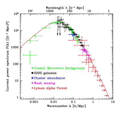
As measurements continue to improve, tests of the inflationary paradigm and specific inflationary models will become more stringent, especially if accurate measurements of the running of the spectral index are performed and tensor perturbations are observed. In addition, an inverse analysis of the observational data may then be attempted, in an effort to directly measure the inflationary “equation of state” hhj . In keeping with the remarkable improvement of observational capabilities, the quality of theoretical predictions has necessarily to be addressed. The central theme of this paper is to quantify and improve the quality of theoretical predictions.
Scalar and tensor power spectra for particular inflation models can be calculated either by direct numerical methods or by employing analytic or semi-analytic approximations such as the slow-roll approach slowrev or uniform approximations hhjm ; hhhjm . For individual models, the numerical approach may well be preferable, but powerful approximations have their own advantages. They provide intuition and understanding applicable to entire classes of models. Provided tight error controls can be met, they are much faster than a mode-by-mode numerical integration for obtaining the power spectrum. Also, both numerical and approximate strategies can be melded together by first obtaining a set of approximate results over a wide range of parameters and then spot-checking numerically. It is our view that both strategies should be applied and compared against each other as they have differing error modes. Finally, it should be kept in mind that the ultimate accuracy with which the primordial fluctuations must be computed is limited by how accurately the radiation and matter transfer functions are known, as well as by the errors associated with observations. At present, the transfer functions can be computed to about accuracy sswz , sufficient for dealing with next-generation observations. We will use this value as a relative figure of merit when discussing errors below. It should be noted that the accuracy requirements for the tensor or gravitational wave component are not as stringent as for the scalar component; the expected signal is at large length scales, where cosmic variance becomes unavoidable. Finally, measurements of the radiation and matter power spectrum at higher values of face issues such as the rapid fall-off of the primary signal, secondary point-source contamination, foreground subtraction (for the CMBR), galaxy bias, systematic errors, effects from baryons baryons and neutrinos aba , and limited accuracy in theoretical computation of the present nonlinear power spectrum codecomp for the matter distribution.
In this paper we focus on the perturbation spectrum for single-field inflationary models. We implement a direct numerical approach as well as the slow-roll and uniform approximations, with the aim of establishing control over the errors associated with each method and understanding their associated advantages and disadvantages. The main technical advances are a robust and numerically efficient strategy for the mode-by-mode integration, simple and useful error estimates for the uniform approximation, and a simple improvement strategy for power spectra amplitudes for the uniform approximation at leading order. We are able to show that the improved leading order uniform approximation leads to very good accuracy for the spectral indices and their running, as well as for the amplitudes of the power spectra and the ratio of tensor to scalar perturbations. For the most part, the accuracy of the results obtained is of the order of .
The method of uniform approximation employed in this paper has been presented in Refs. hhjm ; hhhjm . This method is a “uniformization” of the well-known Wentzel-Kramers-Brillouin (WKB) or Liouville-Green (LG) approximation lg in the presence of transition points. The uniform approximation began with the work of Langer langer and others, and was followed by the notable contributions of Olver olverpap1 ; Olver which we rely on for our analysis below. While this line of investigation rested on the analysis of ordinary differential equations, equivalent asymptotic results based on an integral representation were given by Chester, Friedman, and Ursell uinteg . The uniform approximation has proven very useful in many applications, e.g., chemical physics cm , the semiclassical limit in quantum mechanics berry , and the quantum-classical transition in quantum cosmology shua . For our purposes, the key advantages of the Olver uniform approximation are that it does away with WKB-like matching conditions jeff (such a procedure fails to indicate the error of the approximation), has controlled error bounds over the entire domain of interest, is systematically improvable, and allows analytic simplifications in special cases of physical interest.
The paper is organized as follows. Section II provides the necessary background regarding the calculation of the primordial power spectra and spectral indices for single field inflation models. In Section III the results from the uniform approximation in leading order are given, while in Section IV the essential equations for the slow-roll approximation are summarized. In Section V we give a detailed description of the numerical determination of the primordial power spectra and spectral indices by solving the mode-equations numerically, in the uniform approximation, and in the slow-roll approximation. We investigate three different examples in Section VI and conclude with a discussion of our results in Section VII.
II Background
The generation of perturbations during inflation is due to the amplification of quantum vacuum fluctuations by the dynamics of the background spacetime. In order to calculate the perturbation spectra for these quantum vacuum fluctuations three steps are necessary: the dynamics of the background spacetime must be determined, the mode equations for the scalar and tensor perturbations must be solved, and finally, the power spectra themselves must be calculated as functions of wave-number . We will briefly outline these three steps in the following; for detailed derivations the reader is refered to the literature slowrev ; ivrevs2 ; LLKCBA ; dodelson .
II.1 Background Equations
For single-field inflationary models, i.e., when inflation is driven by a single homogeneous scalar field, the dynamical equation for the inflaton field is given by
| (1) |
The dots denote derivatives with respect to physical time . The evolution of the Hubble parameter , where is the scale factor, is given by the Friedmann equation
| (2) |
Equivalently, by taking the derivative of with respect to time and inserting the equation of motion (1) for we can write
| (3) |
Here and in the following we have set . Eqns. (1) and (2) or (3) determine the evolution of the inflaton field completely. In addition, it is useful to calculate the number of expansion e-folds via
| (4) |
Monitoring the number of e-folds for which inflation lasts allows us to select observationally relevant inflationary models and their parameters. Finally, the conformal time is defined by
| (5) |
As explained later, the uniform approximation is expressed naturally in terms of the conformal time.
Once the background equations are solved we can proceed to the next step, the evaluation of the scalar and tensor perturbations.
II.2 Mode Equations, Power Spectra, Spectral Indices, and their Running
The modern understanding of fluctuations generated by inflation is based on the gauge-invariant treatment of linearized fluctuations in the metric and field quantities ivrevs2 ; givb ; givs ; ivrevs1 . A particularly convenient quantity for characterizing the perturbations is the intrinsic curvature perturbation of the comoving hypersurfaces givdhl , , where is a gauge-invariant scalar perturbation ivrevs2 , and , where is the sound speed and is the curvature of spatial sections. For single-field inflationary models, this simplifies to . The quantity satisfies the dynamical equation
| (6) |
where primes denote derivatives with respect to conformal time and is the spatial Laplacian in comoving coordinates. It follows immediately that is approximately constant in the long wavelength limit . This is true during the inflationary phase as well as during the post-reheating era. Moreover, the Einstein equations can be used to connect the gravitational potential and so that a computation of the power spectrum of provides all the information needed (aside from the transfer functions) to extract the temperature anisotropy of the CMBR. Details of this procedure can be found in Refs. ivrevs2 ; ms .
The calculation of the relevant power spectra involves a computation of the two-point functions for the appropriate quantum operators, e.g.,
| (7) |
the operator being written as
| (8) |
where are annihilation and creation operators with , and . The complex amplitude satisfies
| (9) |
Solving Eqn. (9) is the fundamental problem in determining the primordial power spectrum. The corresponding mode equation for tensor perturbations is given by
| (10) |
Once the mode equations are solved for different momenta the power spectra for the scalar and tensor modes are obtained via
| (11) | |||
| (12) |
where we denote the power spectrum for by .
The tensor power spectrum is often defined with an additional factor as
| (13) |
leading to the definition of the tensor to scalar ratio as
| (14) |
The generalized spectral indices for the scalar and tensor perturbations are defined to be
| (15) | |||||
| (16) |
Running of the spectral indices is conventionally parameterized by the second logarithmic derivative of the power spectra:
| (17) | |||||
| (18) |
Numerical results for the power spectrum are often fit in the literature assuming a power-law behavior and a small running of the spectral index around a pivot scale (see e.g., Refs. LLKCBA ; LLMS ). This fitting ansatz for the power spectrum is
| (19) |
the fitting parameters being , and . The spectral index is evaluated at the pivot scale:
| (20) |
The running is parameterized by . This fitting form is not self-consistent since it is not possible to have strictly constant and non-zero given the above definitions. This inconsistency manifests itself by the uncontrolled growth of errors away from the pivot scale.
In the following we will describe how to obtain approximate solutions for the scalar and tensor power spectra and the spectral indices and their running, assuming that the evolution of the background quantities is known.
III The Uniform Approximation
In two recent papers hhjm ; hhhjm we have implemented an approach based on the uniform approximation (for a detailed description of the approximation, see Ref. Olver ) to calculate the power spectra and the associated spectral indices of primordial perturbations from inflation. Our method leads to simple expressions for the power spectra and spectral indices with calculable error bounds. The solution for the modes can in principle be determined to arbitrary order in the uniform approximation. In practice, results accurate to sub-percent level are obtained at next-to-leading order.
While a detailed derivation of the mode equations, power spectra, and spectral indices with the corresponding error terms is given in Ref. hhhjm , for completeness and to set notation, we provide a brief summary of the main equations. In addition, we give an expression for the scalar to tensor power spectrum ratio with the corresponding error term and explain how to compute the error terms in the uniform approximation in an efficient way. A new result, shown here, is that a simple improvement of the leading order uniform approximation leads to very good accuracy, generically better than . This improvement is obtained by utilizing knowledge of the next-to-leading order results without actually implementing them fully.
III.1 The Mode Functions
In order to solve for the scalar and tensor mode functions in the uniform approximation, it is necessary to rewrite the differential equations (9) and (10) in the following form:
| (21) |
where , and
| (22) |
where . The shift of in the definition of and is necessary in order to have a convergent error control function hhhjm . In the following we will describe the analysis for the scalar modes and present only the final results for the tensor modes.
The general solution for is a linear combination of the two fundamental solutions and , viz.,
| (23) |
independent of the order of the approximation. To fix the coefficients and , a linear combination of and must be taken so that in the limit . With proper normalization, the solution for is, in leading order,
| (24) |
with
| (25) | |||||
| (26) |
One part of the solution is valid to the left of the turning point , defined as the solution to , and the other part is valid to the right of the turning point (). The uniform approximation allows us to calculate bounds on the errors. We write
| (27) |
where the error term encapsulates the contribution to beyond leading order. As derived in detail in Ref. hhhjm , the error term is bounded by
| (28) | |||||
where denotes the total variation of the error control function . A numerical estimate shows Olver . The error control function reads
| (29) | |||||
The limit defines the region of interest for calculating power spectra and the associated spectral indices. In this region, the pole dominates the behavior of the solutions and the Airy solution goes over to the LG form leading to simple expressions for the spectral indices hhhjm . The region of interest lies to the right of the turning point where the argument of the Airy functions becomes large. This allows the approximation of the Airy functions in terms of exponentials, leading to
| (30) | |||||
For computing the power spectra in the limit, only the growing part of the solution is relevant:
| (31) |
In a similar fashion the results for the tensor modes can be derived. We have
| (32) |
where indicates that we replace with and with in Eqn. (25).
Having obtained expressions for the scalar perturbations and the tensor perturbations we can now derive the corresponding scalar and tensor power spectra.
III.2 The Power Spectra
The expression for the scalar power spectrum as defined in Eqn. (11) in the uniform approximation with the corresponding error term is
| (33) | |||||
with
| (34) |
where denotes the power spectrum for the scalar perturbations in the leading order approximation. We can now substitute either the full expression for given in Eqn. (24) or the LG form from Eqn. (31).
Using the LG expression for we have
| (35) |
with the error term for the power spectrum given in Eqn. (34). The calculation for the tensor power spectrum follows along the same lines, yielding
| (36) |
with the error term in the same form as in Eqn. (34) with the substitution .
The tensor to scalar ratio, , is given by
| (37) |
with the error term
| (38) |
In the case of power-law inflation, where is constant, the error is identically zero, as in this case . In other words, the ratio of tensor to scalar perturbations for power-law inflation is exact already at leading order in the uniform approximation.
III.3 Estimate of the Error Bound
Although we can calculate the error bound for the power spectra from the general expressions in Eqns. (28) and (29), it is convenient to have simpler estimates for the errors.
We begin by considering the case of constant , where the -independent error bound for the power spectrum in leading order of the uniform approximation is Olver
| (39) |
the generic denoting either of or . This bound is rigorous and useful, though the prefactor is not optimally sharp for the case of constant .
Suppose now that varies slowly with time. Fix and consider the value of at the turning point , defined by . Given the slow variation of , this value is a slowly varying function of . By expanding the expression for the error control function of Eqn. (29) locally around the turning point, we obtain what is in effect a derivative expansion for the error term. The leading term in this expansion, which is free of derivatives, has the same form as the expression above for constant , though it now carries the mild -dependence of the variable case,
| (40) |
This bound is not meant to be rigorous, since higher order terms in the derivative expansion are not included. However, it is effective and useful in the case of slowly varying . For further discussion of local approximations of this type, see also Section III.5.2. In Ref. hhhjm we have extensively discussed how a non-constant gives rise to a non-vanishing and -dependent error for the spectral index.
III.4 Improvement of the Leading Order Result
In this section we present a new improvement for the leading-order uniform approximation. In previous work hhhjm we derived next-to-leading order results for and and the corresponding power spectra and spectral indices. The resulting expressions contained several integrals, which are tedious to evaluate. On the other hand, the results at next-to-leading order for the case of constant turned out to be very simple. In essence, higher order terms in the uniform approximation generate a prefactor which occurs in the Stirling series for temme
| (41) |
which we know a-priori to be present in the case of constant . This all-orders prefactor improves the normalization of the power spectrum dramatically.
The natural question arises as to whether or not it is possible to utilize these results to improve the leading order expressions without recourse to full computation of the sub-leading approximations. For most viable inflationary models, varies slowly and corrections from the derivatives of are sub-dominant. The full next-to-leading order machinery may not be required if is sufficiently well-behaved. In this section we implement this idea and derive improved leading-order results for the power spectra. Note that, at leading order, the spectral index is exact for constant , thus the main improvement to be expected is in the amplitude of the power spectrum.
We begin with an argument from our previous work hhhjm , which was used to understand why the leading-order result for the spectral index was much more precise than estimated bounds for the power spectrum such as given in Eqn. (40) would seem to indicate. The error is in fact dominated by an amplitude prefactor which has only a subdominant contribution to the spectral index. We split the scattering potential in the form
| (42) |
and choose the -independent but -dependent constant to be the value of at the turning point. As argued previously hhhjm , this splitting allows us to identify two separate contributions to the total error term for the power spectrum,
| (43) |
The term arises solely from the ultra-local contribution in the derivative expansion of , and by explicit calculation it is known to be of the form
The remaining error term satisfies an integral equation of the form considered by Olver Olver , with a reduced inhomogeneity; explicit calculation leads to the rigorous bound
| (45) |
where is the full error control function, is the error control function for the case of constant , and indicates total variation as before.
In the generic case of slowly varying this expression clearly shows that is significantly reduced in comparison to . Therefore we are motivated to absorb the ultra-local contributions from higher order corrections into the power spectrum, leading to an improved first-order expression
| (46) |
This improvement applies to both the scalar and tensor power spectra, with and respectively. Since typical values of occur for both scalar and tensor fluctuations, the terms on the right hand side of Eqn. (46) correspond to amplitude corrections of order , , , and , respectively. These can be viewed primarily as local normalization corrections.
To complete the discussion, we can obtain a non-rigorous estimate for the size of , again using a derivative expansion in to isolate the leading local contributions. In this expansion, the leading derivative-free terms in must cancel, and therefore the leading term is proportional to the first derivative of . After some calculation we find
| (47) | |||||
where we have used the chain rule to write the derivative in terms of a derivative of with respect to and have used the explicit form for . It is understood that this is not a rigorous inequality, since we have neglected the higher order terms in the derivative expansion, but it is well-motivated and useful for slowly-varying . This error estimate determines the order to which the local corrections (46) should be taken into account. For instance, when is slowly varying, most of the error can be compensated using Eqn. (46). Examples will be encountered in Section VI, where we explicitly demonstrate the success of this improvement procedure. As is to be expected, the ratio is much less sensitive to the normalization error compared to the amplitude of the power spectrum. For this quantity, the error is well-estimated by Eqn. (47).
III.5 The Spectral Indices
We now turn to the evaluation of spectral indices and corresponding error terms from the power spectra computed using the uniform approximation. We will discuss further simplifications leading to local expressions for and .
III.5.1 Integral Expression for the Spectral Index
The differentiation of the power spectrum with respect to is straightforward. As stated earlier, it is important to remember that the turning point is a function of since where is the value of at the turning point . Using this relation, we find
| (48) |
The error for the spectral index only arises from the -dependent part of the error in the power spectrum. Therefore, the error in the spectral index is sensitive only to the time variation of . To estimate this error, the spectral index as written in Eqn. (15) can be expressed via the leading order power spectrum in the following form:
| (49) | |||||
with
| (50) |
where we estimate by the leading order error term in Eqn. (42), i.e., by as given in Eqn. (III.4). It should be noted that the leading errors in the spectral index are proportional to derivatives of , unlike the situation for the power spectrum [Eqn. (III.4)].
The above analysis can be carried out for tensor perturbations in an identical fashion, including the error estimation, with the replacement . The spectral index for gravitational waves is given by
| (51) |
III.5.2 The Local Approximation
It is possible to simplify the expressions for the spectral indices as given in Eqns. (48) and (51) by approximating the integrals further. By doing so, we lose the ability to quantify the error estimates for and but are able to write down local expressions for the spectral indices. The integrands in Eqns. (48) and (51) have square-root singularities at the turning points, i.e., at the lower integration limits. At the upper limit, goes to zero and the integrands vanish linearly, therefore, assuming and , respectively, are well-behaved, we expect the main contribution to the integrals to arise from the lower limit. Using the knowledge that and are slowly varying, we expand them around their turning points in Taylor series. To second order in derivatives,
| (52) |
where a bar indicates that the quantity has to be evaluated at the turning point. For we obtain a similar expression with the index replaced by . We can now solve the integrals in Eqns. (48) and (51) exactly and find for the scalar spectral index
and for the tensor spectral index analogously
The local approximation is a further simplification of the leading order result in the uniform approximation and we will test its accuracy with three numerical examples in Section VI. We denote the leading contribution of unity in the curly brackets in Eqns. (III.5.2) and (III.5.2) as zeroth order, the second term proportional to as first order in the local approximation, and the remaining terms proportional to and as second order.
III.5.3 Spectral Indices in Terms of Slow-Roll Parameters
It is possible to simplify the expressions for the spectral indices one step further and obtain results similar to the ones obtained in the slow-roll approximation to be discussed in the next section. We have investigated this further approximation in detail previously hhhjm and pointed out its shortcomings. Here the results are summarized for leading order only.
We begin by considering the spectral index for the scalar perturbations as given in Eqn. (III.5.2). In order to write in terms of slow-roll parameters which are defined as (see e.g., Ref. sg )
| (55) |
we expand , , and up to second order in these parameters. The contribution is already of fourth order and is neglected. Using the expression for conformal time in slow-roll parameters given by
| (56) |
the relation, , and
| (57) |
it is easy to write down and its derivatives in terms , , and (For a detailed derivation and explicit expressions, see Ref. hhhjm ). As in earlier sections, the bar indicates that the parameters are to be calculated at the turning point. Inserting all the expressions into the local approximation for the scalar spectral index, Eqn. (III.5.2), allows us to write the spectral index in terms of slow-roll parameters:
Equivalently, for the tensor spectral index derived from a slow-roll expansion of the local result, Eqn. (III.5.2), we find
| (59) |
where we have used
| (60) |
Compared to results given previously hhjm ; hhhjm , the expressions for the spectral indices given here have been fully expanded to second order in slow-roll parameters.
IV The Slow-Roll Approach
The most popular analytic method to evaluate primordial power spectra and spectral indices is the so-called slow-roll approach. The basic idea behind this approach is the following. Recall the expression for in terms of , and as given in Eqn. (57). Assume now that and are small and constant. If this is the case, all terms vanish, since they can be written as derivatives of and , and all terms of order can be neglected. It is then also possible to express as , leading to a simplified equation for :
| (61) |
with
| (62) |
This equation is immediately solved in terms of Bessel functions. Since the constant will be different for different values of (as and are approximated by different constants for different ), for every momentum a “best-fit power-law” result is obtained and expressions for the power spectrum and the spectral index can be derived. Tensor perturbations can be treated in the same way, leading to expressions for and . The terminology “slow-roll” is easy to understand: the requirement on and being small and roughly constant admits inflationary models with smooth potentials, leading to a phase where the inflaton field rolls slowly down the potential before inflation ends and reheating begins. The shortcoming of the slow-roll approach is that there is no simple way to improve the approximation beyond leading order. Once the assumption that the slow-roll parameters are constant is given up, at the next formal order of the approximation, the Bessel solution is no longer valid wms . Different ways for improving the slow-roll approximation have been suggested, e.g., sg ; srimprov ; CGS ; gong , but they often lead to rather involved expressions for power spectra and spectral indices and, more importantly, are not error-controlled.
As the slow-roll approach is convenient, widely used, and for most common inflationary models expected to be a reasonable approximation, we will compare slow-roll results against the exact mode-by-mode integration and the uniform approximation in Section VI. For completeness, we summarize here the results for the power spectra and spectral indices following closely the work of Stewart and Lyth sl .
The power spectra in the slow-roll approximation read
| (63) | |||||
| (64) |
where is the Euler-Mascheroni constant, and .
The scalar and tensor spectral indices are given by
| (65) | |||||
| (66) |
and . The expressions and are the well-known first-order slow-roll results.
In the numerical calculations for slow-roll presented below, we will approximate the solutions of the mode equations in terms of Bessel functions, while solving the background equations without any further approximations. Hence, we do not assume the strict slow-roll conditions that the slow roll parameters , , and be constant. This is not the way the slow-roll approach is often implemented when estimating inflationary parameters: A further asymptotic approximation is utilized to solve the background equations salbond ; LPB employing a derivative expansion in the inflationary potential . Such expansions may provide useful estimates but do not give the precision required by present and upcoming CMBR observations. The reason for the inaccuracy arising from expansions in the potential, as will be seen in an example, is that the Taylor expansion in derivatives can often fail. This is not the case when the parameters are expressed in terms of the Hubble parameter and its derivatives. Our aim here is to determine the accuracy of the mode solutions themselves, therefore we do not focus on errors arising from approximations to the background equations.
V Numerical Implementations
In this section we describe the numerical implementation of the exact mode-by-mode integration and the uniform approximation and its simplifications. Technical details can be found in Appendix A. Since the uniform approximation is useful both in setting initial conditions for the exact numerical solution, and as a complete semi-analytic method in its own right, we discuss it first below.
V.1 Leading Order Uniform Approximation: Numerical Issues
V.1.1 Preliminaries
We begin by addressing some technical points and introducing conventions. Since the conformal time is defined only up to a constant, we set it to zero at the end of inflation. If the given model does not have a natural end to inflation this point is somewhat arbitrary and we set to zero typically some number of e-folds after the highest mode of interest freezes out.
The power spectrum and the spectral indices are to be calculated in the limit , so that the LG approximation can be used. To avoid accumulation of numerical error, however, these quantities should not be calculated directly in this limit. Since the freeze-out happens soon after the turning point is crossed, the computation is carried out some e-folds after the turning point for each respective mode, but well before the end of inflation. The linear combination of both solutions to the mode equations, in terms of Ai- and Bi-functions, is then completely dominated by the exponentially growing part. We found that carrying out the computations 4 or 5 e-folds after the respective turning point provided sufficient accuracy.
In all the computations described below, the Ai- and Bi-functions were calculated with the algorithm given in Ref. airynums .
V.1.2 The Mode Solutions
The full solutions and are not needed for the calculation of the power spectrum and the spectral index. Nevertheless, it is useful to calculate some of them for selected momenta in order to compare the leading order uniform solutions to the exact numerical solutions found from a mode-by-mode integration of the differential equations. For we can calculate the integrals appearing in , as defined in Eqn. (25) numerically via
| (67) |
where is an initial value of the conformal time. In the actual numerical routine we therefore have to know the second integral before we can calculate the uniform solutions left of the turning point: This is achieved by an additional run of the integrator for the background equations.
V.1.3 Power Spectra and Spectral Indices
The power spectra for scalar and tensor perturbations in leading order of the uniform approximation are given by Eqns. (35) and (36). The integrals are calculated using a trapezoidal rule with non-equidistant discretization in conformal time. As mentioned above, we avoid calculating the spectra numerically in the limit , but instead do so some 4-5 e-folds after the turning point. In the case of power-law inflation analytical results are available for the leading order contributions to the power spectra (see Ref. hhhjm ). We have checked that the power spectra numerically calculated from Eqns. (35) and (36) are in agreement with these analytic results (see Section VI.1 and Table 1 for details).
The spectral indices in the uniform approximation may be calculated either by numerically differentiating the power spectrum as described in Section III.5 for the exact mode-by-mode approach, or by using the formulae in Eqns. (48) and (51). In Appendix A.2 we describe how to deal with the inverse square root singularities appearing in the integrals to be performed in the second case.
V.2 Mode-by-Mode Numerical Integration
V.2.1 Initial Conditions and Mode Functions
In order to numerically obtain the mode functions, we must satisfy the initial condition requirement, i.e., in the limit ,
| (68) |
Two difficulties in imposing this formal initial condition immediately arise. First, in any numerical solution, the calculation must begin at a finite initial time, thus for modes with small enough values of , the condition may not be fulfilled. Second, for modes at larger values, there are very many oscillations before the turning point is reached, naively requiring very fine time-steps if the entire temporal range must be handled numerically.
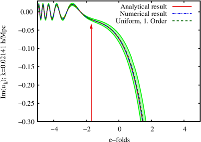
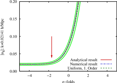
To circumvent these problems, we use the uniform approximation to set initial conditions in a regime where it is exponentially accurate. For each mode, we take as initial condition the uniform approximation result at roughly 20 zeros, i.e., 10 oscillations, before the turning point for that mode. The number of zeros from a given time to the turning point can be estimated by . As shown below, this initialization procedure suppresses numerical errors, especially in the high regime where the precision of the power spectrum and the spectral index is improved without taking smaller and smaller time steps. In addition, only a smaller number of “active” modes, i.e., the modes that are within some 20 zeros before the turning point and not yet frozen, need be considered at any time. In the regime of small , we first note that as inflation has to start somewhere in practical numerical calculations, this introduces a lowest value for , defined by the criterion that the mode should be well inside the Hubble length. As the initial conditions for inflation are unknown, we will assume (i) that inflation began well before the 55-65 e-folds necessary to solve the flatness and horizon problems, and (ii) by the time our calculations are to be performed, Eqn. (68) applies. By isolating how initial conditions are defined from possible early-time artifacts, our method of implementing initial conditions also leads to substantial improvement in the low- regime as well.
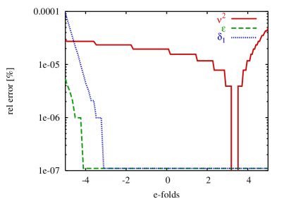
In Figs. 2 and 3 we display the imaginary (growing) part and absolute value of for a mode with for a power-law inflation model. As can be seen in both cases, the uniform approximation at leading order and the numerical results are clearly very close. The error in the absolute value (relevant to the power spectrum) from the mode-by-mode integration is shown in Fig. 4. The numerical error is less than 1 part in . To check the accuracy of the solution of the background equations, the numerical deviations from the expected pure constant values for , , and are shown in Fig. 5; the errors are comfortably below parts per million. Detailed quantitative results are given in the following section.
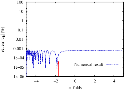
V.2.2 Power Spectra and Spectral Indices
For the case of scalar perturbations the modes freeze out once the power spectrum , as defined in Eqn. (11), becomes constant as a function of conformal time, i.e., when at a numerically determined freeze-out time . We found that it is numerically robust to track the time derivative of to determine this freeze-out. The same situation holds for the tensor perturbations and as defined in Eqn. (12).
Once the power spectra have been obtained, the spectral indices for scalar and tensor perturbations are found by evaluating the derivatives of the power spectra with respect to , as defined in Eqns. (15) and (16). The derivatives are computed numerically with nonequidistant momentum discretization due to the momentum readjustment described in Appendix A.1. We take three discretization points and approximate the derivative by a non-symmetric, second-order, rule. In the numerical evaluation of the derivatives, for every individual we use two very close neighboring points with – over the entire -range considered.
VI Results
In this section we discuss three inflation models. We start with power-law inflation, one of the very few analytically solvable cases. Next we investigate two chaotic inflation models, with a quadratic and quartic potential, respectively. Finally, we present a model in which the third derivative in the potential does not exist at one point, leading to a “kink” in .
We present below results from numerical solution of the mode equations, the uniform approximation with different simplifications and improvements, and slow-roll approximations in first and second order. In all cases, we show the results for the ratio of tensor and scalar power spectra, as well as the scalar and tensor spectral indices. Some of the results are presented in tables, for a specific value of the momentum , while selected results are shown in figures. In addition to the basic quantities themselves, we also give relative errors in some cases.
VI.1 Power-Law Inflation
| Approximation | |||||
|---|---|---|---|---|---|
| Analytical | 1.454545 | 0.8 | 0 | -0.2 | 0 |
| Numerical111mode-by-mode integration | 1.454544 | 0.79998 | -0.20002 | ||
| Uniform, 1. order222already exact in that order | 1.454541 | 0.79992 | 0.00001 | -0.20008 | 0.00001 |
| Local approx., 0. order222already exact in that order | – | 0.80000 | -0.20000 | ||
| Local approx., 1. order222already exact in that order | – | 0.79999 | -0.20001 | ||
| Uniform, Slow-Roll redux333see Eqn. (III.5.3) and Eqn. (59) | – | 0.80165 | -0.19835 | ||
| Slow-Roll, 1. order444expected results: and | 1.454545 | 0.81818 | -0.18182 | ||
| Slow-Roll, 2. order555expected results: and | – | 0.80165 | -0.19835 | ||
As one of the few analytically tractable models, power-law inflation MatRatra provides a useful foil for testing approximations. This feature has maintained its popularity, even though the basic model is not realistic, as inflation never comes to an end. We compared detailed results from the uniform approximation in leading and next-to-leading order with slow-roll and exact results previously hhhjm : The spectral index was exact already in leading order in the uniform approximation, while the slow-roll approximation yields a Taylor expansion of the spectral index. The amplitude of the power spectrum in the uniform approximation was accurate to roughly 10% in leading order while in next-to-leading order the accuracy of the amplitude improved dramatically with an error smaller than 1%. These results hold for widely differing values of , the power in the time evolution of the expansion [the potential is )]. In contrast, the slow-roll approximation being an expansion in , has large errors for small , decreasing as increases.
Here, we use the power-law model for testing the accuracy of our numerical implementations of the exact mode equations, as well as the uniform and slow-roll approximations. The spectral indices are constant, therefore the running of the spectral index – which measures the -dependence of and – vanishes. In addition, the ratio of the power spectra is constant. Instead of showing our results graphically – all curves would be almost indistinguishable by eye – we summarize our findings in Table 1. We quote the results for , the spectral indices, and their running and at the WMAP pivot scale spergel . We have picked the power , which is of course much too small to be considered a realistic inflationary model, but is perfectly acceptable for illustrative purposes. In the uniform approximation there is an explicit expression for the spectral indices and , while the tensor to scalar ratio is calculated via the amplitudes of the power spectra. In the purely numerical computation, the spectral index is obtained by taking numerical derivatives of the power spectrum as as described earlier.
The error in the exact numerical determination of the ratio of the power spectra is smaller than 1 part in , while the numerical error in the implementation of the uniform approximation is slightly larger (3 parts in ). In the case of power-law inflation, the spectral indices do not accurately reproduce the expected analytic results, though they do reproduce the expected slow-roll results to -order with the slow-roll parameters being constant in time (in this case, and ). This provides a check on the integration of the background equations, but has no further useful information.
For the scalar spectral index we find a relative error in the exact numerical calculation of while for the uniform approximation the relative error is roughly . Again, no error in the numerical implementation of the slow-roll approximation is detected. The situation for the tensor spectral index is similar. The numerical errors in the uniform approximation for the spectral indices are slightly larger than for the exact numerical mode-by-mode approach due to the numerical integration of a function with an inverse square root singularity. The results for and are very close to zero in all cases.
In addition, we tested our improvement strategy for the uniform approximation which should work perfectly in the case of power-law inflation since is constant. We found a relative error for of if we include corrections up to , of including corrections up to , and of if we include corrections up to following Eqn. (46). The corrections are slightly worse than anticipated but consistent with the small error in the numerical implementation of the uniform approximation.
VI.2 Chaotic Inflation
| Approximation | |||||
|---|---|---|---|---|---|
| Numerical111mode-by-mode integration | 0.13749 | 0.96507 | -0.00064 | -0.01765 | -0.01779 |
| Uniform, 1. order | 0.13740(14) | 0.96505(3) | -0.00064 | -0.01768(1) | -0.01773 |
| Uniform, improved 1. order222the improvement here is to second order in powers of , Cf. Eqn. (46) | 0.13749(0) | 0.96507(0) | -0.00064 | -0.01765(0) | -0.01773 |
| Local approx., 0. order333see Eqn. (III.5.2) and (III.5.2) | – | 0.96465 | -0.00066 | -0.01786 | -0.01799 |
| Local approx., 1. order333see Eqn. (III.5.2) and (III.5.2) | – | 0.96501 | -0.00064 | -0.01761 | -0.01770 |
| Uniform, Slow-Roll redux444see Eqn. (III.5.3) and Eqn. (59) | – | 0.96566 | -0.00062 | -0.01757 | -0.01768 |
| Slow-Roll, 1. order555see Eqn. (65) and (66) | 0.13752 | 0.96523 | -0.00063 | -0.01741 | -0.01755 |
| Slow-Roll, 2. order555see Eqn. (65) and (66) | – | 0.96507 | -0.00064 | -0.01764 | -0.01779 |
(a)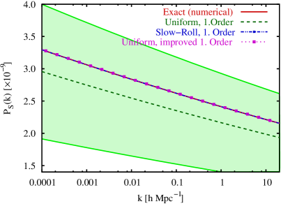 (b)
(b)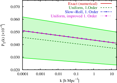
Next we study two chaotic inflation models. In these examples, the slow-roll approach is expected to work well; in order to obtain enough e-folds of inflation the potentials cannot be very steep, thus slow-roll turns out to be a very good approximation. For the uniform approximation we expect similar results as for the power-law case: an accuracy more or less independent of the chosen parameters.
VI.2.1 Quadratic Potential:
(a)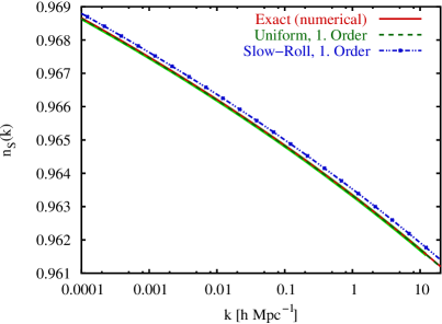 (b)
(b)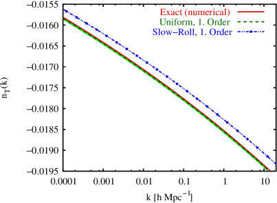
The simplest chaotic model is that for a free scalar field with mass . In this model, normalizing the amplitude of the scalar power spectrum to the WMAP fit, as described in Appendix A.3, is equivalent to fixing . The initial value for the inflaton field is given by with a small initial velocity of . These parameters ensure that the inflationary phase lasts long enough to provide a realistic model, i.e., it leads to 57.655 e-folds after the mode crosses the Hubble length.
First, we analyze the results for the power spectra and , plotted in Figs. 6a and 6b. The exact numerical results for the power spectra as defined in Eqns. (11) and (12) are shown in red (solid line), the results from the leading order uniform approximation given in Eqns. (35) and (36) are shown in green (dashed line), the first order slow-roll results as defined in Eqns. (63) and (64) are shown in blue (dashed-dotted line), and the improved uniform approximation results [to second-order in the sense of Eqn. (46) for the scalar perturbations] are shown in purple (dotted line). The light green band displays our estimate of the error bound for the leading order uniform approximation as given in Eqn. (40). The error estimate for the improved uniform approximation in leading order [see Eqn. (47)] is so close to the result itself that the error band is not visible in this plot. We will use these color and linestyle assignments for the remainder of the paper.
| Approximation | |||||
|---|---|---|---|---|---|
| Numerical111mode-by-mode integration | 0.25963 | 0.94999 | -0.00090 | -0.03356 | -0.01705 |
| Uniform, 1. order | 0.25948(113) | 0.94990(3) | -0.00089 | -0.03367(2) | -0.01694 |
| Uniform, improved 1. order222the improvement here is to second order in powers of , Cf. Eqn. (46) | 0.25964(0) | 0.94999(0) | -0.00089 | -0.03356(0) | -0.01703 |
| Local approx., 0. order333see Eqn. (III.5.2) and (III.5.2) | – | 0.94942 | -0.00092 | -0.03395 | -0.01726 |
| Local approx., 1. order333see Eqn. (III.5.2) and (III.5.2) | – | 0.94991 | -0.00090 | -0.03340 | -0.01697 |
| Uniform, Slow-Roll redux444see Eqn. (III.5.3) and Eqn. (59) | – | 0.95081 | -0.00087 | -0.03368 | -0.01706 |
| Slow-Roll, 1. order555see Eqn. (65) and (66) | 0.25969 | 0.95077 | -0.00087 | -0.03285 | -0.01669 |
| Slow-Roll, 2. order555see Eqn. (65) and (66) | – | 0.95001 | -0.00089 | -0.03354 | -0.01703 |
The exact numerical results, the improved leading order uniform approximation, and the slow-roll approximation are almost indistinguishable by eye in Fig. 6. The leading order uniform approximation deviates in the amplitude from the exact numerical result by as expected. The improvement strategy performs just as predicted by Eqn. (46): the second-order correction reduces the error to while the fourth-order reduces it further to , for both scalar and tensor perturbations. This consistently good behavior is due to the fact that is varying slowly. Note that the improvement strategy should be carried out to roughly match the error estimate given by Eqn. (47) – fourth-order in this instance; beyond this point the error is dominated by other contributions.
Next we investigate the scalar and tensor spectral indices as functions of . The results are displayed in Figs. 7a and 7b. The shaded band represents the error estimate for the leading order of the uniform approximation [see Eqn. (50), calculated with the estimate in Eqn. (III.4)]. The error estimate for the scalar spectral index is of the order , therefore of the same order as the discrepancy to the numerical result. Note that the improved scalar and tensor spectral index calculations, following the discussion in Section III.5.1, agree completely with the numerical results in Table 2. The deviation of the slow-roll approximation for the scalar spectral index in first order from the exact numerical result is also very small, roughly . As stated before this is not surprising: the slow-roll approximation is expected to work well for this type of model, where the slow-roll parameters and are very small and almost constant. However, the tensor spectral index has an error of more than .
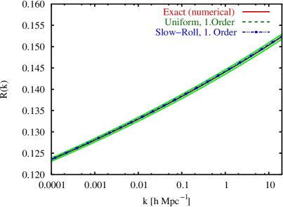
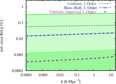
In Fig. 8 the ratio of tensor to scalar perturbations as defined in Eqn. (14) is shown. The corresponding relative errors of the uniform approximation, of the slow-roll approximation, and of the improved uniform approximation are presented in Fig. 9. In Fig. 8 the lines representing the different approximations are practically indistinguishable by eye. In contrast to the relative errors in the power spectra ( without improvement and with fourth-order improvement), the relative error in the tensor to scalar ratio is already smaller than (dashed line in Fig. 9) without the improvement, and smaller than , i.e., practically exact, with second-order improvement (solid line in Fig. 9) (Cf. Section III.4). There is no point in improving further since the result has already reached the estimated error threshold (47) beyond which improvement becomes incomplete. This behavior is a general feature of the approximation when the inflation model leads to a slowly varying .
Finally, we have listed the ratio of tensor to scalar perturbations, the scalar and spectral spectral index, and their running in the various approximations or simplified approximations (introduced in Section III.5), in Table 2. All quantities are again evaluated at . Error estimates for the uniform approximation are indicated by the numbers in brackets. For chaotic inflation the running of the spectral indices, and is non-zero. Note that the running of the tensor spectral index is roughly an order of magnitude bigger than the running of the scalar spectral index.
VI.2.2 Quartic Potential:
(a)
 (b)
(b)
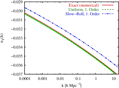
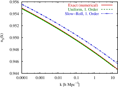
In the quartic model – relative to the quadratic potential – higher derivatives of the potential exist. Consequently, the slow-roll results in this case are expected to have a bigger error. In comparison to the quadratic case, for the model considered below, the errors are worse for the scalar spectral index ( versus ) and comparable for the case of the tensor spectral index (). In contrast, the uniform approximation still provides an accuracy of a fraction of a percent. Although the slow-roll expansion for this model can be improved to second-order with notably better results, this behavior exhibits the general tendency of the slow-roll expansion if terms arising from higher order derivatives of the potential are significant. In terms of observational viability, the -model is under strong pressure from combined analysis of the WMAP CMBR anisotropy data and data from galaxy clustering (see e.g., Refs. Peiris ; LeachLiddle ; Tegmark:2004qd ).
The results for the spectral indices are displayed in Figs. 10a and 10b. As in the previous example the leading-order uniform approximation is very close to the exact numerical results. However, the first-order slow-roll result does not match as closely as for the quadratic potential. As done earlier for the -model, we have listed the various characteristic quantities in Table 3.
VI.3 Inflationary Model with a -Potential Function
As the last example we investigate a toy model with a continuous potential function with continuous first and second derivatives and a jump in the third derivative at a specific value of . Generally speaking, dynamical changes in the potential of the field driving inflation can be induced by couplings to other degrees of freedom. For example, in hybrid models a phase transition is used to terminate inflation. If a dynamical transition happens at cosmologically relevant scales, i.e., well before the end of inflation, it leaves a clear signature in the power spectra and spectral indices. Such a transition may be naturally realized in multi-field models of inflation (see e.g., Ref. Hunt:2004vt ). Other examples are steps in the potential (see e.g., Ref. wms ; Adams:2001vc ), leading to oscillations in the primordial power spectra and spectral indices. In such models cannot be considered as a constant, but can display sudden changes.
(a)
 (b)
(b)
(a)
 (b)
(b)
Rather than taking one of the potentials mentioned above we consider here a toy potential that is smoother in the sense that oscillations in or are avoided:
| (69) | |||||
| (70) |
where for and for . The potential is constructed in such a way that , and but . Thus there is a finite jump in the third derivative of the potential.
We present numerical results with parameters chosen specifically to demonstrate the general effect of a more rapidly changing . During the evolution in this potential the parameters and are not constant (not even approximately); cannot be considered small when the inflaton field fulfills (with the parameters below, can be as large as ).
The parameters chosen to specify the model are: , , , , . With this choice of parameters the number of e-folds counted from is .
(a)
 (b)
(b)
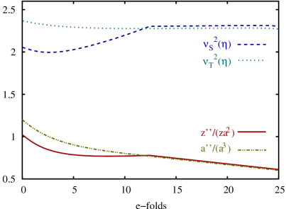
The relevant time-dependent terms and in the scalar and and in the tensor mode equations are displayed in Fig. 11 as a function of expansion e-folds ( and have been divided out by to filter out the exponential growth of the scale factor). The point is reached at (note that in this plot defines the beginning of the numerical calculation). Due to the jump in the third derivative both quantities for the scalar perturbations display a kink at this point. The qualitative behavior is also different on either side of the kink. While has a kink, is completely well-behaved. Note that , as e.g., expressed in Eqn. (57) as an exact expression in terms of the slow-roll parameters, is more sensitive to higher derivatives of the potential than [Cf. Eqn. (60)]. Thus we can expect the effects of the change in the potential at to be amplified in the scalar power spectrum relative to the tensor power spectrum.
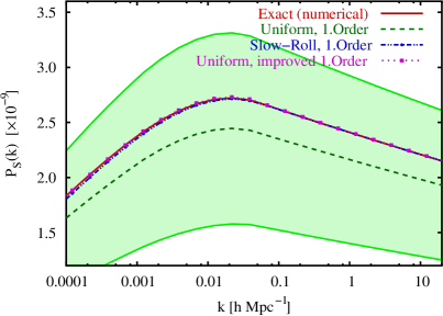
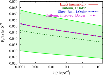
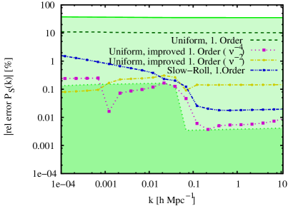
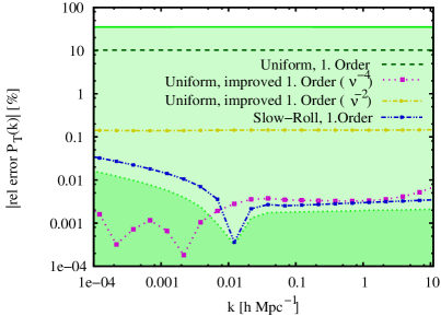
The results for the scalar and tensor power spectrum are displayed in Figs. 12a and 12b. With the same conventions as in Fig. 6, the different approximations (leading and improved leading order of the uniform approximation and the slow-roll approximation) are compared to the exact numerical results. The scalar power spectrum (see Fig. 12a) shows a significant deviation from a power-law shape. Up to the spectrum rises, reaches a maximum and falls off for larger . As in the previous examples, the leading order of the uniform approximation has an amplitude error of roughly with respect to the exact numerical results. The (second-order) improved leading order uniform approximation, however, lies almost on top of the numerical results. Remarkably, although the shape deviates from a simple power-law behavior quite significantly, the improvement strategy is still effective.
The relative errors are shown in Figs. 13a and 13b. The error behavior divides into two regimes, to the left and the right of Mpc-1. The behavior to the right is that of a -model [Cf. Eqn. (69)] while the behavior to the left is that of a polynomial potential with linear, quadratic, and quartic terms (70). Note that the error estimate from Eqn. (47) changes sharply across this divide, by more than an order of magnitude, from to . To the left, this error estimate shows that there is no point in attempting a correction beyond second-order using Eqn. (46), consistent with the results shown for second and fourth-order corrected spectra. To the right, the smallness of the error estimate is consistent with the improved quality of the fourth-order results. Results for the tensor spectrum are qualitatively similar. As expected, the uniform approximation improves on the slow-roll result to the left of Mpc-1, since the slow-roll assumptions are violated in this region.
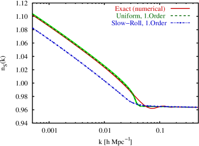
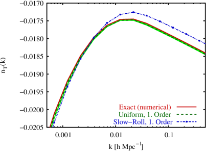
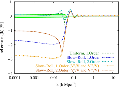
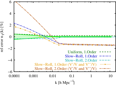
The spectral indices are displayed in Figs. 14a and 14b. The potential (see Fig. 11) leads to a blue scalar spectrum for smaller momenta and a red scalar spectrum for larger momenta (Fig. 14a). For the spectral index the uniform approximation in leading order is remarkably close to the exact numerical result, more or less independent of . It only deviates slightly at for the scalar spectral index. In Fig. 15 the relative errors of the uniform approximation and the slow-roll approximation are displayed. Away from the transition -value, the relative error is smaller than for the scalar spectral index and smaller than for the tensor spectral index. The slow-roll approximation, by comparison, deviates by from the exact numerical results.
(a)
 (b)
(b)
In all the computations so far, the background equations were not approximated to obtain and and its derivatives, but were solved numerically. Based on a Taylor expansion in the potential and its derivatives, Liddle and Lyth LL92 introduced an approximation for the background equations. This approach (formalized and expanded to higher orders by Liddle, Parsons, and Barrow LPB ) leads to a simplification of the slow-roll parameters in the following form:
| (71) | |||||
| (72) | |||||
Here we have followed the conventions of Stewart and Lyth sl . Being an asymptotic expansion, this approximation can sometimes lead to extra errors. For the last model, we have calculated the spectral indices with this additional approximation and the degradation in relative error is shown in Fig. 15.
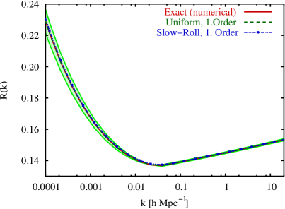
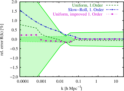
The ratio of tensor to scalar perturbations is depicted in Fig. 16, while the corresponding relative errors for the different approximations are shown in Fig. 17. The uniform and the slow-roll approximation are both quite close ( error) to the exact numerical result, even though the variations in are not small. Following Section III.4 the accuracy of the leading-order uniform approximation for the ratio can be improved using Eqn. (46) and the corresponding equation for tensor perturbations. We have not displayed this improved ratio in Fig. 16, since it would be almost indistinguishable from the exact numerical result. However, Fig. 17 shows that the relative error of the second-order improved leading order of the uniform approximation is smaller than over the whole -range, consistent with the error estimate (47).
VI.4 Consistency relations
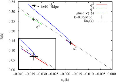
Single field inflation is characterized by degeneracies in the observable parameters, such as the tensor to scalar ratio , the scalar spectral index , the tensor spectral index , and their respective running. Not all the parameters are independent; they are connected by so-called “consistency relations.” For power-law inflation, e.g., the tensor spectral index is related to the scalar spectral index via the special result . In the context of slow-roll inflation, consistency relations between, e.g., and have been derived (see e.g., Ref. LL92 for an early derivation, note, however, that Liddle and Lyth define as the ratio of the quadrupole moments. Since this definition introduces further uncertainties through the transfer functions here we use the amplitudes of the power spectra themselves). A more general expectation beyond slow-roll is that is some function of and .
Following Ref. LLKCBA we introduce rescaled amplitudes via
| (73) | |||||
| (74) |
leading, in the first order slow-roll expansion, to a consistency relation between and of the form:
| (75) |
Or, adapted to our notation,
| (76) |
The equality in this relation is only valid when the first-order slow-roll quantities are used, even for power-law inflation. Note also that the relation is -dependent in general.
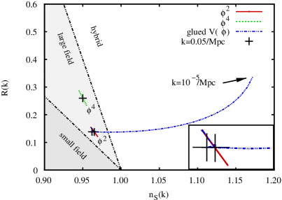
Inspired by the idea of consistency relations between measurable quantities from the microwave background, Dodelson et al. Dodelson:1997hr classified inflationary models depending on the relative magnitudes of the spectral indices and , and the ratio of the amplitudes of the power spectra . In terms of slow-roll parameters, the classification is based on the relative magnitudes of and . Using Eqn. (76), relations between slow-roll parameters can be translated to inequalities between and . The three model types are then characterized by:
-
(i)
Small field models:
or ,
-
(ii)
Large field models:
or ,
-
(iii)
Hybrid models:
or .
In Fig. 18 we show as a function of for the three models investigated in the previous sections. The -dependence, i.e., the running of the quantities, produces lines, rather than single points in the plane. For the single-field chaotic models these lines are straight. This is not the case, however, for the -potential where the -dependence is not a straight line, but a curve. For all three models we have marked the location of the central pivot with a cross. In all cases the total number of e-folds is fixed to be counted from the pivot scale.
We can also test the consistency relation of slow-roll inflation. In Fig. 19, is plotted as a function of . The slow-roll dominated chaotic models are indeed very close to the slow-roll consistency relation (the dotted line in Fig. 19), but not the -model. A detailed understanding of the consistency relations and their observational value requires further study.
Regarding observations, the allowed range in the - plane is already constrained by WMAP, the SDSS Galaxy clustering information and the SDSS Ly forest measurements (see e.g., Ref. Tegmark:2004qd ). An observation of parametric degeneracy by future CMBR experiments, e.g., PLANCK PLANCK , would provide strong support for inflation as the source of primordial fluctuations.
VII Conclusions
In this paper we have presented different approaches to the computation of primordial power spectra and the corresponding spectral indices and their running, with a view to understanding and controlling the various sources of error in the calculations. In addition, the ratio of the tensor to scalar power spectra and the related consistency relation were investigated.
We have implemented an efficient and accurate method for exact mode-by-mode integration utilizing results from the uniform approximation to set up the initial conditions. The uniform approximation, introduced for calculating inflationary perturbations in hhjm ; hhhjm , was numerically investigated in detail. We showed that the leading order results in this approximation for the power spectrum can be easily improved for well-behaved and using previously obtained results for the case of constant (the results for the spectral indices and are already excellent and do not need to be improved). Our numerical and semi-analytic results for the power spectra and spectral indices agree within . Thus, the primordial power spectra can be determined at the same level of accuracy as the transfer functions.
A key feature of the uniform approximation is the existence of an error control theory, which is missing in the slow-roll approximation. At leading-order in the uniform approximation, we showed how to implement a useful approximate error bound for the power spectrum. In addition, we provided an error estimate for the power spectra obtained from the improved first order uniform approximation and the spectral indices. These error estimates are based on our knowledge of the ultra-local corrections from the second order uniform approximation results. Thus, these estimates are much tighter than the general leading order error bounds from the uniform approximation.
We have analyzed in detail three different classes of inflationary models: power-law models, chaotic models, and a model with a -potential. We used the power-law model, for which exact analytical results exist, to demonstrate the accuracy of our numerical implementations of the exact mode-by-mode integration, the uniform approximation, and the slow-roll approximation. The deviation of the analytic and numerical results was in general very small, around 1 part in . Two scale-free chaotic inflationary models were chosen as representatives for common slow-roll models: For these models the slow-roll approximation was excellent. As a final example, we constructed a -potential which had two dynamical phases patched together in a relatively smooth manner. In the first phase, where changes more rapidly than in the second phase, the uniform approximation was much more accurate than the slow-roll approximation, while in the second phase both approximations produced very good results with small errors.
Up-coming high-precision CMBR measurements will provide data to constrain the zoo of inflation models. An accurate and fast code for calculating primordial power spectra, spectral indices, and their running will be crucial to this analysis. We are developing an interface to connect our code to Boltzmann solvers cmbfast in order to generate the ’s directly. In addition, we will use the code to test the robustness of the information obtained on the inflationary equation of state from the measured power spectrum by our recently introduced non-parametric reconstruction program hhj . These two complementary approaches provide new precision probes of the first moments of our Universe.
VIII Acknowledgments
The authors thank Scott Dodelson for useful discussions and encouragement to write a code for exact mode-by-mode integration. We are grateful to Max Tegmark for permission to reproduce Fig. 1. AH gratefully acknowledges the warm hospitality and stimulating atmosphere at the Los Alamos National Laboratory (LANL). AH thanks Jürgen Baacke for helpful discussions and continuous encouragement. The work of AH at LANL has been supported by a DAAD short-term scholarship for graduate students and by the University of Dortmund. This research is supported by the Department of Energy, under contract W-7405-ENG-36.
Appendix A Numerical Implementation Details
A.1 Comment on the Momentum Discretization
The actual momentum discretization chosen for numerical work is arbitrary but it is a good idea to adjust the chosen values of the momenta so that the relation
| (77) |
defining the momentum-dependent turning points is satisfied exactly, even though the conformal time is known only at discrete points. This can be done by locking the momentum discretization to the time discretization, i.e., by guaranteeing that if the time discretization is given, discretization points are chosen only if they satisfy Eqn. (77). Of course a predefined momentum discretization is unnecessary if we only wish to calculate power spectra and spectral indices in the uniform approximation; the predefined momentum discretization is used only for initializing the mode functions in the mode-by-mode approach, where we need the integrals on the left of the turning point.
A.2 Spectral Indices in the Uniform Approximation
The integral for the spectral index has a square root singularity at and is handled specially in the numerical routine. We split the integral appearing in the spectral index into two parts:
where is a small quantity. Note that is really dependent, because the discretization in is not equidistant.
In the first integral we can substitute by , i.e., insert the leading order of the local approximation. The first integral can then be calculated analytically and keeps track of the inverse square root singularity, while the second integral has no singularity and can be easily calculated numerically. The quantity is given by the actual time discretization in physical time that we have chosen. It is further required that , i.e., be sufficiently small. As in the limit , this relation also constrains the highest reliable mode for a given time discretization in the exact numerical results. The first integral gives
| (79) | |||||
In order to avoid calculating the integrals numerically up to , we calculate the remainder of the integral from an asymptotic value , where the integrand is sufficiently small and we can stop the numerical integration, to , assuming that . Then we have
| (80) |
with
| (81) |
Alternatively, it is possible to convert the evaluation of the spectral index into the problem of solving a differential equation, rather than evaluating an integral. The limit in Eqn. (48) is interchangeable with a conformal time derivative, so that the physical time derivative of the spectral index reads
| (82) |
In order to avoid the square root singularity the integration starts at , so that the “initial” condition
| (83) |
includes the integral in Eqn. (79). It is understood that the limit is taken when calculating . The integration of the differential equation with a high order integrator is more precise than a standard trapezoidal rule. In contrast, as the discretization in is not equidistant, higher-order integration schemes would be somewhat more complicated to implement. However, we have verified that a standard trapezoidal integration rule already gives sufficiently precise answers. In fact, the local approximation for the spectral index at leading order is quite close to the numerical nonlocal integral in the cases where the derivative expansion is valid.
A.3 Conversion to Physical Units
For completeness, we explain here how units are handled in the numerical implementation. As always, it is convenient to work in dimensionless units, i.e., by choosing . In addition, we set the factor in the Friedmann equation in the numerical code to unity. These choices lead to values for the input parameters, e.g., initial conditions and coupling constants, of order unity. This helps prevent numerical problems arising from very large or very small numbers. In order to reconvert the dimensionless units to physical units the Hubble parameter has to be rescaled via
| (84) |
where is the dimensionless Hubble parameter used in the code and . The rescaled momentum in physical units is therefore given by
| (85) |
with . The initial expansion rate is . Throughout the paper we have dropped the suffix “phys” implying that all results are given in physical units.
Next we discuss the normalization of the amplitude of the power spectrum. The power spectra for scalar and tensor perturbations as defined in Eqns. (11) and (12) are dimensionless and therefore not sensitive to the units of . Their amplitude is determined fully by the parameters chosen in the inflaton potential . Since parameters such as the inflaton mass in a chaotic -model are generally not known, we present the results for the power spectra with respect to the WMAP normalization where the amplitude of scalar perturbations is given by with (at Mpc), see Refs. verde ; spergel . Using the fact that for a fixed number of e-folds, counted from the horizon crossing of , the parameters in the monomial potentials simply lead to a global normalization factor ivrevs2 we can avoid having very small numbers in the numerical calculations and just normalize the spectra afterwards. When stating results we give in each case the parameters in the potential corresponding to the WMAP normalization.
References
- (1) A.H. Guth, Phys. Rev. D 23, 347 (1981).
- (2) V. Lukash, Pis’ma Zh. Eksp. Teor. Fiz. 31, 631 (1980) [JETP Lett. 31, 596 (1980)]; V.F. Mukhanov and G.V. Chibisov, Pis’ma Zh. Eksp. Teor. Fiz. 33, 549 (1981) [JETP Lett. 33, 532 (1981)]; Zh. Eksp. Teor. Phys. 83, 475 (1982) [Sov. Phys. JETP 56, 258 (1982)]; A.H. Guth and S.-Y. Pi, Phys. Rev. Lett. 49, 1110 (1982); S.W. Hawking, Phys. Lett. B 115, 295 (1982); A.A. Starobinsky, Phys. Lett. B 117, 175 (1982).
- (3) C.B. Netterfield et al., ApJ 571, 604 (2002); N.W. Halverson et al., ApJ 568, 38 (2002); A. Benoit et al., AA 399, L19 (2003); T.J. Pearson et al., ApJ 591, 556 (2003); C.-l. Kuo et al., ApJ 600, 32 (2004).
- (4) e.g., W.J. Percival et al., MNRAS 327, 1297 (2001); K. Abazajian et al. [SDSS Collaboration], Astron. J. 128, 502 (2004).
- (5) P. McDonald et al., arXiv:astro-ph/0407377.
- (6) M. Tegmark et al., Astrophys. J. 606, 702 (2004).
- (7) S. Habib, K. Heitmann, and G. Jungman, arXiv:astro-ph/0409599.
- (8) A.R. Liddle and D.H. Lyth, Cosmological Inflation and Large-Scale Structure (Cambridge, 2000) and references therein.
- (9) S. Habib, K. Heitmann, G. Jungman, and C. Molina-París, Phys. Rev. Lett. 89, 281301 (2002).
- (10) S. Habib, A. Heinen, K. Heitmann, G. Jungman, and C. Molina-París, Phys. Rev. D 70, 083507 (2004).
- (11) U. Seljak, N. Sugiyama, M. White and M. Zaldarriaga, Phys. Rev. D 68, 083507 (2003).
- (12) M. J. White, Astropart. Phys. 22, 211 (2004); H. Zhan and L. Knox, arXiv:astro-ph/0409198.
- (13) K. Abazajian, E. R. Switzer, S. Dodelson, K. Heitmann and S. Habib, arXiv:astro-ph/0411552.
- (14) K. Heitmann, P.M. Ricker, M.S. Warren, and S. Habib, astro-ph/0411795.
- (15) G. Green, Trans. Camb. Phil. Soc. 6, 457 (1837); J. Liouville, J. Math pures appl. 2, 16 (1837).
- (16) R.E. Langer, Trans. Amer. Math. Soc. 33, 23 (1931); 34, 447 (1932); 36, 90 (1934); 37, 397 (1935); 67, 461 (1949); Phys. Rev. 51, 669 (1937); T.M. Cherry, Trans. Amer. Math. Soc. 68, 224 (1950).
- (17) F.W.J. Olver, Philos. Trans. R. Soc. A 247, 307 (1954).
- (18) F.W.J. Olver, Asymptotics and Special Functions, (AKP Classics, Wellesley, MA 1997).
- (19) C. Chester, B. Friedman, and F. Ursell, Proc. Camb. Philos. Soc. Math. Phys. Sci. 53, 599 (1957); B. Friedman, J. Soc. Indust. Appl. Math. 7, 280 (1959).
- (20) J.N.L. Connor and R.A. Marcus, J. Chem. Phys. 55, 5636 (1971).
- (21) M.V. Berry, Philos. Trans. R. Soc. 287, 237 (1977).
- (22) S. Habib, Phys. Rev. D 42, 2566 (1990).
- (23) H. Jeffreys, Proc. Lond. Math. Soc. 23, 428 (1924). For applications to inflation, see J. Martin and D.J. Schwarz, Phys. Rev. D 67, 083512, (2003); R. Casadio, F. Finelli, M. Luzzi and G. Venturi, arXiv:gr-qc/0410092.
- (24) V.F. Mukhanov, H.A. Feldman, and R.H. Brandenberger, Phys. Rep. 215, 203 (1992).
- (25) E. Lidsey, A.R. Liddle, E.W. Kolb, E.J. Copeland, T. Barreiro, and M. Abney, Rev. Mod. Phys. 69, 373 (1997).
- (26) S. Dodelson, Modern Cosmology (Academic Press, 2003) and references therein.
- (27) J.M. Bardeen, Phys. Rev. D 22, 1882 (1980).
- (28) For a readable account of gauge invariant perturbations, see J.M. Stewart, Class. Quant. Grav. 7, 1169 (1990).
- (29) H. Kodama and M. Sasaki, Prog. Th. Phys. Supp. 78, 1 (1984).
- (30) D.H. Lyth, Phys. Rev. D 31, 1792 (1985).
- (31) J. Martin and D.J. Schwarz, Phys. Rev. D 57, 3302 (1998); 62, 103520 (2000).
- (32) S.M. Leach, A.R. Liddle, J. Martin and D.J. Schwarz, Phys. Rev. D 66, 023515 (2002).
- (33) N. Temme, Special Functions, p. 66, (John Wiley & Sons, Inc., New York, 1996).
- (34) E.D. Stewart and J.-O. Gong, Phys. Lett. B 510, 1 (2001).
- (35) L. Wang, V.F. Mukhanov, and P.J. Steinhardt, Phys. Lett. B 414, 18 (1997).
- (36) E.D. Stewart, Phys. Rev. D 65, 103508 (2002).
- (37) J. Choe, J.O. Gong, and E.W. Stewart, JCAP 0407, 012 (2004).
- (38) J.O. Gong, Class. Quant. Grav. 21, 5555 (2004).
- (39) E.D. Stewart and D.H. Lyth, Phys. Lett. B 302, 171 (1993).
- (40) S. Zhang and J. Jin, Computation of Special Functions, (John Wiley & Sons, Inc., New York, 1996).
- (41) J.A. Adams, B. Cresswell and R. Easther, Phys. Rev. D 64, 123514 (2001).
- (42) D.S. Salopek and J.R. Bond, Phys. Rev. D 42, 3936 (1990).
- (43) A.R. Liddle, P. Parsons, and J.D. Barrow, Phys. Rev. D 50, 7222 (1994).
- (44) F. Lucchin and S. Matarrese, Phys. Rev. D 32, 1316 (1985); B. Ratra, Phys. Rev. D 45, 1913 (1992).
- (45) D.N. Spergel et al. [WMAP Collaboration], Astrophys. J. Suppl. 148, 175 (2003).
- (46) H.V. Peiris et al., Astrophys. J. Suppl. 148, 213 (2003).
- (47) S. M. Leach and A. R. Liddle, Phys. Rev. D 68, 123508 (2003).
- (48) M. Tegmark, arXiv:astro-ph/0410281.
- (49) P. Hunt and S. Sarkar, Phys. Rev. D70, 103518, 2004.
- (50) A.R. Liddle and D.H. Lyth, Phys. Lett. B 291, 391 (1992).
- (51) S. Dodelson, W.H. Kinney, and E.W. Kolb, Phys. Rev. D 56, 3207 (1997).
- (52) URL: http://www.rssd.esa.int/index.php?project=PLANCK
- (53) URL: http://www.cmbfast.org; U. Seljak and M. Zaldarriaga, Ap. J. 469, 437 (1996); URL: http://camb.info, A. Lewis, A. Challinor, and A. Lasenby, Ap. J. 538, 473 (2000).
- (54) L. Verde et al., Astrophys. J. Suppl. 148, 195 (2003).