Redshift-Space Distortions with the Halo Occupation Distribution I: Numerical Simulations

Abstract

We show how redshift-space distortions of the galaxy correlation function or power spectrum can constrain the matter density parameter $\Omega_{m}$ and the linear matter fluctuation amplitude $\sigma_{8}$. We improve on previous treatments by adopting a fully non-linear description of galaxy clustering and bias, which allows us to achieve the accuracy demanded by larger galaxy redshift surveys and to break parameter degeneracies by combining large-scale and small-scale distortions. Given an observationally motivated choice of the initial power spectrum shape, we consider different combinations of $\Omega_{m}$ and $\sigma_{8}$ and find paramters of the galaxy halo occupation distribution (HOD) that yield nearly identical galaxy correlation functions in real space. We use these HOD parameters to populate the dark matter halos of large N-body simulations, from which we measure redshift-space distortions on small and large scales. We include a velocity bias parameter $\alpha_{v}$ that allows the velocity dispersions of satellite galaxies in halos to be systematically higher or lower than those of dark matter. Large-scale distortions are determined by the parameter combination $\beta\equiv\Omega_{m}^{0.6}/b_{g}$, where $b_{g}$ is the bias factor defined by the ratio of galaxy and matter correlation functions, in agreement with the linear theory prediction of parameter degeneracy. However, linear theory does not accurately describe the distortions themselves on scales accessible to our simulations. We provide fitting formulas to estimate $\beta$ from measurements of the redshift-space correlation function or power spectrum, and we show that these formulas are significantly more accurate than those in the existing literature. On small scales, the “finger-of-god” distortions at projected separations $\sim 0.1$ $h^{-1}$Mpc depend on $\Omega_{m}\alpha_{v}^{2}$ but are independent of $\sigma_{8}$, while at intermediate separations they depend on $\sigma_{8}$ as well. One can thus use measurements of redshift-space distortions over a wide range of scales to separately determine $\Omega_{m}$, $\sigma_{8}$, and $\alpha_{v}$.

1 Introduction

In a universe that obeys the cosmological principle, the clustering of galaxies is statistically isotropic. But in galaxy redshift surveys the distances to galaxies are inferred from redshifts, making the line of sight a preferred direction. Peculiar velocities produce anisotropy in redshift-space clustering on all scales. On small scales, the random motions of galaxies in virialized systems stretch groups and clusters into so-called “fingers-of-god” (FOG). On large scales, coherent flows created by gravity compress overdense regions along the line of sight and stretch underdense regions correspondingly. Small and large scale distortions provide diagnostics for the matter density parameter $\Omega_{m}$ and the amplitude of mass fluctuations (Peebles 1976; Sargent & Turner 1977; Kaiser 1987). In this paper and its companion, we develop techniques for modeling redshift-space distortions that draw on recent developments in the theory of galaxy clustering. These techniques are designed to reach the level of accuracy demanded by the new generation of large galaxy redshift surveys, such as the Two-Degree Field Galaxy Redshift Survey (2dFGRS; Colless et al. 2001) and the Sloan Digital Sky Survey (SDSS; York et al. 2000).

In the linear theory model of Kaiser (1987), the relation of the anisotropic, redshift-space galaxy power spectrum $P_{Z}(k,\mu)$ to the isotropic, real-space galaxy power spectrum $P_{R}(k)$ is

$$P_{Z}(k,\mu)=P_{R}(k)(1+\beta\mu^{2})^{2},$$ (1)

where $\mu$ is the cosine of the angle between the wavevector ${\bf k}$, and the line of sight. The amplitude of the distortion is determined by $\beta=\Omega_{m}^{0.6}/b_{\rm lin}$, where the linear bias parameter $b_{\rm lin}\equiv\delta_{g}/\delta_{m}$ is assumed to be independent of scale ($\delta_{g}$ and $\delta_{m}$ represent galaxy and mass density contrasts, respectively). Fourier transformation of equation (1) gives expressions for the galaxy correlation function in redshift space, $\xi(r_{\sigma},r_{\pi})$ (Hamilton 1992).

Unfortunately, non-linear effects make equation (1) inaccurate on all scales where observations yield precise measurements (Cole, Fisher, & Weinberg 1994). The effects of non-linearity can be approximated by a phenomenological model in which galaxies have, in addition to linear theory distortions, random small scale velocities drawn from an exponential distribution with dispersion $\sigma_{v}$ (Peacock & Dodds 1994; Park et  al. 1994; Cole et  al. 1995). In this model, the Kaiser formula becomes

$$P_{Z}(k,\mu)=P_{R}(k)(1+\beta\mu^{2})^{2}(1+k^{2}\sigma_{v}^{2}\mu^{2}/2)^{-2}.$$ (2)

In practice, most estimates of $\beta$ from large-scale redshift-space distortions have utilized this linear-exponential model, expressed in terms of the power spectrum as in equation (2) or in terms of the correlation function or spherical harmonics. The current state-of-the-art measurement is the analysis of the 2dFGRS presented by Hawkins et  al. (2003), yielding $\beta=0.49\pm 0.09$, updating the earlier 2dFGRS analysis of Peacock et  al. (2001). Previous observational efforts and theoretical developments are expertly reviewed by Strauss & Willick (1995) and Hamilton (1998).

The essential limitation of equation (2) is that it is derived from an unphysical model. There are several sources of non-linearity in redshift-space distortions in addition to small scale dispersion (Cole et  al. 1994; Fisher & Nusser 1996), and the dispersion itself is correlated with the local density and is not a constant for all galaxies. Scoccimarro (2004) shows that the velocity distribution corresponding to the linear-exponential model is itself unphysical, containing a $\delta$-function and a discontinuity at the origin, and that equation (2) does not become fully accurate even at very large scales. Hatton & Cole (1999) concluded that this model introduces a $\sim 15\%$ systematic error in the determination of $\beta$, which is significant compared to the precision achievable with 2dFGRS and the SDSS. Furthermore, the $\sigma_{v}$ parameter, while related to the amplitude of the small scale distortions, has no clearly defined physical meaning. In redshift-space distortion analyses it is purely a nuisance parameter, significantly degenerate with $\beta$, and has no use in constraining cosmological parameters.

The program initiated by Kaiser (1987) largely supplanted an earlier tradition of using small-scale redshift distortions to constrain $\Omega_{m}$ via the “cosmic virial theorem” (Peebles 1976, 1979; Davis, Geller, & Huchra 1978; Bean et  al. 1983). The analytic expression of this “theorem” relied on the assumption of stable clustering, which early N-body simulations showed was unlikely to hold on the relevant scales (e.g., Davis et al. 1985). A more serious problem is that the bias between galaxy and dark matter clustering is likely to have a complex effect on quantities that enter the cosmic virial theorem, one that cannot be captured by a single bias parameter with an obvious physical interpretation.

The goal of this paper and its companion is to present techniques for physical modeling of redshift-space distortions that can take advantage of high-precision measurements on large and small scales. We construct these techniques in the framework of the Halo Occupation Distribution (HOD; see, e.g. Ma & Fry 2000; Peacock & Smith 2000; Seljak 2000; Benson 2001; Scoccimarro et  al. 2001; Berlind & Weinberg 2002; Cooray & Sheth 2002), in which the bias of a specified class of galaxies is defined by the probability distribution $P(N|M)$ that a halo of mass $M$ contains $N$ galaxies, together with prescriptions for spatial and velocity bias within individual halos. The HOD has proven to be a powerful tool for encapsulating the bias predictions of galaxy formation models (Kauffmann et  al. 1997; Benson et  al. 2000; White et  al. 2001; Yoshikawa et  al. 2002; Berlind et  al. 2003; Kravtsov et  al. 2004; Zheng et  al. 2004), for analytic calculations of galaxy clustering statistics (see Cooray & Sheth 2002 and numerous references within), and for empirical modeling of galaxy clustering data (Jing et  al. 1998; van den Bosch et  al. 2003; Zehavi et  al. 2004a,b; Yang et  al. 2004; Mo et  al. 2004; Abazajian et al. 2004; Tinker et al. 2004). Several recent papers have presented calculations of redshift-space distortions or peculiar velocity statistics using halo models of dark matter and galaxy clustering (Seljak 2001; White 2001; Sheth et al. 2001; Sheth & Diaferio 2001; Kang et  al. 2002; Cooray 2004), providing insight into the role of non-linear dynamics and non-linear bias in shaping clustering and anisotropy. However, these studies primarily focus on dark matter rather than galaxy clustering, and they have not yet yielded a clear blueprint for constraining cosmological parameters with HOD modeling of observed redshift-space distortions, which is our objective here.

We use the HOD formulation to set up the redshift-space distortion problem in the following terms. Any redshift survey large enough to yield useful measurements of large-scale anisotropy will first allow precise measurements of the projected correlation function, $w_{p}(r_{p})$, which is unaffected by peculiar velocities. For any choice of cosmological parameters, one should choose HOD parameters to reproduce this measurement of real-space clustering. If an acceptable fit cannot be found for the given cosmology, then the model is already ruled out (e.g. Abazajian et  al. 2004). For models with acceptable real-space clustering, one calculates redshift-space distortions using numerical simulations or analytic approximations to test the model’s cosmological parameters. In practice, the parameters that enter are $\Omega_{m}$ and the amplitude of the linear theory matter power spectrum $P_{\rm lin}(k)$, which we characterize by $\sigma_{8}$, the rms linear matter fluctuation in 8 $h^{-1}$Mpc spheres (with $h\equiv H_{0}/100$ km s^-1 Mpc^-1). We assume that the shape of $P_{\rm lin}(k)$ is known from measurements of the large scale galaxy power spectrum and cosmic microwave background (CMB) anisotropy, which together pin down the parameters that determine $P_{\rm lin}(k)$ quite accurately (e.g., Percival et al. 2002; Spergel et al. 2003; Tegmark et al. 2004a). Since redshift-space anisotropy is insensitive to the shape of $P_{R}(k)$ — in equations (1) and (2) the $\mu$-dependence of $P_{Z}(k)$ factors out entirely — small uncertainties in the shape of $P_{\rm lin}(k)$ should have minimal effect. In this work we adopt the power spectrum form of Efstathiou, Bond, & White (1992), where the shape is parameterized by the characteristic wavenumber $\Gamma$.

While matching $w_{p}(r_{p})$ can constrain HOD parameters relevant to real-space clustering, we must also allow for the possibility that galaxies in a halo have a systematically different velocity dispersion from that of the halo dark matter. (The mean velocity of galaxies and dark matter within a halo should be the same because both components feel the same large-scale gravitational field.) Numerical simulations predict that the galaxy closest to the halo center of mass moves at nearly the center of mass velocity while satellite galaxies have a velocity dispersion similar to that of the dark matter (Berlind et al. 2003; Faltenbacher et al. 2004). We define the satellite “velocity bias”, $\alpha_{v}$, as the ratio between these two dispersions. Although the numerical simulations predict that $\alpha_{v}\approx 1$, this parameter could depart modestly from unity as a result of dynamical friction, tidal disruption or mergers of slowly moving satellites, or different orbital anisotropy of galaxies and dark matter. We will treat $\alpha_{v}$ as a free parameter to be constrained by the observations, but we will assume that it is constant over the relevant range of halo masses. We will also consider effects of non-zero velocities for central galaxies, though simulations predict these velocities to be $\la 20\%$ of the virial velocity.

In this paper we use N-body simulations to create halo populations for a set of cosmological models, and we populate those halos with galaxies using HOD models that yield similar real-space clustering. We examine the constraints that redshift-space distortions can impose within the three-dimensional parameter space ($\Omega_{m}$, $\sigma_{8}$, $\alpha_{v}$), and we use our numerical results to obtain fitting formulas that can estimate parameters from observational data. In a companion paper, we develop a numerically calibrated analytic model for redshift-space distortions. The analytic model provides physical insight into the numerical results, and it can make more complete use of the observational measurements for cosmological parameter estimation.

In Section 2 below, we describe the numerical simulations and the HOD models used to populate them with galaxies. Section 3 presents an overview of redshift-space anisotropies in the two-dimensional correlation function $\xi(r_{\sigma},r_{\pi})$. In §4 we focus on measures of large-scale distortion based on multipole decomposition of the power spectrum and the correlation function. These measures mainly constrain the parameter combination $\beta\equiv\Omega_{m}^{0.6}/b_{g}$, which can be related to $\sigma_{8}\Omega_{m}^{0.6}$ using the measured (real-space) galaxy clustering. (As discussed in §4.4, we define $b_{g}$ by a ratio of non-linear correlation functions, which makes it similar but not identical to the linear theory bias factor $b_{\rm lin}$.) In §5 we turn to small scale distortions, which most directly constrain $\Omega_{m}\alpha_{v}^{2}$ and have some power to break degeneracies further and yield separate determinations of $\Omega_{m}$, $\sigma_{8}$, and $\alpha_{v}$. In §6 we summarize our results and discuss how they can be applied to cosmological parameter estimation from observational data.

Table 1: Properties of the Simulations and HOD Parameters

$z_{\rm out}$	$\Omega_{m}$	$\sigma_{8}$	$b_{g}$	$M_{\rm min}$ [$h^{-1}$M⊙]	$M_{1}$ [$h^{-1}$M⊙]	$\alpha$
0	0.100	0.950	0.922	3.73$\times 10^{11}$	9.38$\times 10^{12}$	0.934
0.19	0.158	0.900	0.956	5.96$\times 10^{11}$	1.45$\times 10^{13}$	0.959
0.56	0.297	0.801	1.041	1.09$\times 10^{12}$	2.51$\times 10^{13}$	1.005
0.97	0.459	0.699	1.181	1.70$\times 10^{12}$	3.51$\times 10^{13}$	1.109
1.45	0.620	0.599	1.358	2.19$\times 10^{12}$	3.99$\times 10^{13}$	1.199

Note. — When we scale an output to a different value of $\Omega_{m}$, the values of $M_{\rm min}$ and $M_{1}$ scale in proportion to $\Omega_{m}$, as discussed in §2.3.

2 Numerical Simulations and HOD Models

2.1 N-body Simulations

We use N-body simulations to create halo populations for a sequence of cosmological models, always assuming a spatially flat universe dominated by cold dark matter and a cosmological constant ($\Lambda$CDM), with Gaussian initial conditions and a primordial power spectrum motivated by observations of CMB anisotropies and large-scale structure.

We choose the mass resolution by requiring that there be at least 30 particles in the lowest mass halos that host simulated galaxies. On this basis we select a mean interparticle separation of $\bar{n}^{-1/3}=0.7$ $h^{-1}$Mpc for all initial conditions. For $\Omega_{m}=0.3$, the 30-particle limit corresponds to a minimum halo mass of $\sim 10^{12}$ $h^{-1}$M_⊙, similar to the minimum halo mass found for the HOD fit (assuming $\Omega_{m}=0.3$) to the SDSS sample of galaxies brighter than $M_{r}=-20+5\log h$ (Zehavi et  al. 2004b). All of our simulated galaxy populations have a space density of $\bar{n}_{g}=5.6\times 10^{-3}$ ($h^{-1}$Mpc)^-3, equal to that of SDSS galaxies brighter than $0.68\,L_{\ast}$ (Blanton et al. 2003), or $M_{r}=-20.04+5\log h$.

To cover the $(\Omega_{m},\sigma_{8})$ parameter space in an efficient manner, we draw on the findings of Zheng et  al. (2002), who demonstrated that changes in $\Omega_{m}$ at fixed $\Gamma$ and $\sigma_{8}$ simply scale halo masses in proportion to $\Omega_{m}$ and halo velocities in proportion to $\Omega_{m}^{0.6}$. In terms of these scaled masses and velocities, the mass function, spatial correlations, and velocity correlations of halos identified at fixed overdensity are virtually independent of $\Omega_{m}$. We can therefore run a single simulation that has a high value of $\sigma_{8}$ at redshift zero and use the earlier redshift outputs to represent $z=0$ results for lower values of $\sigma_{8}$. For each $\sigma_{8}$, the halo population can be scaled to any desired value of $\Omega_{m}$. Specifically, we run simulations with $\Omega_{m}=0.1$ and $\sigma_{8}=0.95$ at $z$=0, and use the outputs at $z$=0.19, 0.56, 0.97, and 1.45 when $(\Omega_{m},\sigma_{8})$ = (0.16, 0.90), (0.30, 0.80), (0.46, 0.70), and (0.62, 0.60). We model different values of $\Omega_{m}$ by scaling the halo masses in proportion to $\Omega_{m}$, the halo velocities by $\Omega_{m}^{0.6}$, and the internal halo velocity dispersions by $\Omega_{m}^{0.5}$. We carry out a test of this scaling in §2.3 to demonstrate that it is accurate enough for our purposes here.

Figure 1: The two power spectra used in the simulations, $\Gamma=0.2$ and $\Gamma=0.12$, are compared to the linear power spectrum computed with CMBFAST using the parameters listed in column 6 of Table 4 in Tegmark et  al. (2004b). All three power spectra are normalized to the same value of $\sigma_{8}$. The fundamental mode of the simulation volume is indicated with the arrow at $k=2\pi/L_{\rm box}=0.025\;h/$Mpc. The $\Gamma=0.2$ power spectrum is similar to the CMBFAST calculation over the range of scales simulated, while the $\Gamma=0.12$ power spectrum has more power at large scales and increasingly less as $k$ increases.

We analyze simulations with two values of the power spectrum shape parameter, $\Gamma=0.2$ and 0.12, both with inflationary spectral index $n_{s}=1$. On the scales probed by our simulations, $\Gamma=0.2$ corresponds well to the power spectrum calculated with CMBFAST (Seljak & Zaldarriaga 1996) with $\Omega_{m}=0.3$, $h=0.7$, and $\Omega_{b}=0.04$, values favored by recent observations (e.g., Spergel et  al. 2003; Tegmark et al. 2004b). The redder, $\Gamma=0.12$ power spectrum corresponds to a lower combination of $\Omega_{m}h$, or a tilted ($n_{s}<1$) primordial spectrum. This model is at the extreme edge of those allowed by current data, so comparing results for $\Gamma=0.2$ and $\Gamma=0.12$ should give a conservative estimate of uncertainties associated with the power spectrum shape. In Figure 1 we compare these two power spectra to one created with the transfer function calculated by CMBFAST using the cosmological parameters listed in Table 4 (column 6) of Tegmark et  al. (2004b), who derive combined constraints from WMAP CMB data, and the SDSS galaxy power spectrum. Each power spectrum is normalized to the same value of $\sigma_{8}$. The fundamental mode of the box is marked with the arrow. Inside this scale, the $\Gamma=0.2$ power spectrum closely tracks the CMBFAST calculation. The $\Gamma=0.12$ $P(k)$ has less small-scale power, but it has significantly more power at scales near the fundamental mode.

We use the publicly available tree-code GADGET (Springel, Yoshida, & White 2000) to integrate the initial conditions. We evolve $360^{3}$ particles in a volume 253 $h^{-1}$Mpc on a side, giving us a mass resolution of $9.66\times 10^{10}\times\Omega_{m}$ $h^{-1}$M_⊙ per particle. The force softening was set to one-tenth the mean interparticle separation, or $\epsilon=70$ $h^{-1}$kpc. The simulations were started at an expansion factor $a=0.01$, with a maximum timestep of 0.005 in $a$. GADGET employs individual particle timesteps governed by a particle’s acceleration, such that $\Delta a\propto\sqrt{\epsilon\eta}$. The value of $\eta$ was set to 0.2. We ran five independent realizations to estimate the sample variance.

We also ran a similar series of simulations using the particle-mesh (PM) technique, with a staggered-mesh algorithm similar to that of Melott (1983) and Park (1990). (The code we use was written by V. Narayanan.) The high efficiency of the PM algorithm allowed us to run simulations with the same mass resolution but box sizes of $324$ $h^{-1}$Mpc per side, twice the volume of our GADGET runs. In comparing the results from the two methods, we found that the lower force resolution of the PM technique (with a $900^{3}$ grid) had a significant impact on the number of halos near our 30-particle resolution limit, while the smaller volume of the GADGET runs did not adversely affect the distortions at large scales. We therefore use the GADGET runs exclusively in our subsequent analyses.

Table 2: Properties of the Mock Galaxy Distributions

[$\Omega_{m},\alpha_{v}$]					[$\sigma_{8},\alpha_{v}$]					[$\beta,\alpha_{v}$]					[$\Omega_{m},\sigma_{8}$]
	$\Omega_{m}$	$\sigma_{8}$	$\beta$			$\Omega_{m}$	$\sigma_{8}$	$\beta$			$\Omega_{m}$	$\sigma_{8}$	$\beta$			$\alpha_{v}$	$\alpha_{vc}$	$\beta$
	0.3	0.95	0.53			0.1	0.8	0.24			0.24	0.95	0.46			0.0	0.0	0.46
	0.3	0.90	0.51			0.2	0.8	0.36			0.26	0.90	0.46			0.8	0.0	0.46
	0.3	0.80	0.46			0.3	0.8	0.46			0.3	0.80	0.46			1.0	0.0	0.46
	0.3	0.70	0.41			0.4	0.80	0.55			0.36	0.70	0.46			1.2	0.0	0.46
	0.3	0.60	0.36			0.5	0.80	0.63			0.47	0.60	0.46			1.0	0.2	0.46

Note. — In the first three sequences, $\alpha_{v}=1$ and $\alpha_{vc}=0$. The HOD parameters and bias factors $b_{g}$ for each value of $\sigma_{8}$ are listed in Table 1.

2.2 HOD Models

To identify halos in the dark matter distribution we use the friends-of-friends algorithm (Davis et  al. 1985) with a linking length of 0.2 times the mean interparticle separation. Objects identified with this linking length typically have an average density of $\rho/\bar{\rho}\sim 200$, which is roughly the criterion for virialization of a collapsed object. Only halos with 30 or more particles were retained in the halo sample.

We need to populate the halos with galaxies in a way that generates similar $\xi_{R}(r)$ for all values of $\sigma_{8}$. We use the HOD parameterization of Kravtsov et  al. (2004) and Zheng et  al. (2004), which was also adopted in the empirical modeling of the SDSS correlation function by Zehavi et  al. (2004b). Halos above a minimum mass $M_{\rm min}$ are assigned one central galaxy. The mean number of satellite galaxies in halos with $M\geq M_{\rm min}$ is

$$\langle N_{\rm sat}\rangle_{M}=\left(\frac{M}{M_{1}}\right)^{\alpha}.$$ (3)

The mean number of galaxies in a halo is therefore $\langle N\rangle_{M}=1+(M/M_{1})^{\alpha}$ for $M\geq M_{\rm min}$ and $\langle N\rangle_{M}=0$ for $M<M_{\rm min}$. We assume Poisson scatter in the number of satellite galaxies with respect to the mean $\langle N_{\rm sat}\rangle_{M}$, consistent with the theoretical predictions of Kravtsov et al. (2004), and Zheng et al. (2004).

We adopt the parameter combination $(\Omega_{m},\sigma_{8})=(0.3,0.8)$ for our central model. To populate the halos in this model, we choose observationally motivated HOD parameters similar to those derived for the SDSS $M_{r}<-20+5\log h$ galaxy sample by Zehavi et al. (2004b). The resulting correlation function is shown by the solid line in Figure 2. For other $\sigma_{8}$ values, we choose $M_{1}$, $\alpha$, and $M_{\rm min}$ so that we closely match $\xi_{R}(r)$ of the central model, while maintaining a fixed galaxy space density. We carry out the HOD parameter fits using the analytic model of $\xi_{R}(r)$ described by Tinker et al. (2004), which refines the model described by Zheng (2004). The cosmological and HOD parameters of our simulations are listed in Table 1.

Figure 2: The real-space galaxy two-point correlation functions for the five cosmologies and HOD parameters listed in Table 1. The inset box shows the different correlation functions normalized by that of the central model, $\Omega_{m}=0.3$, $\sigma_{8}=0.8$. The error bars in the inset box are those for the central model. Results are averaged over five realizations, and error bars show the run-to-run dispersion divided by $\sqrt{N-1}=2$ to calculate the error in the mean. In both panels, the dash-dotted line is the correlation function for the central model’s cosmological and HOD parameters but the $\Gamma=0.12$ initial power spectrum.

We assume that satellite galaxies trace the dark matter distribution within halos; a test in §3 below shows that our results are insensitive to this assumption (see Figure 7). Instead of selecting random dark matter particles from the friends-of-friends halos, we randomly place satellite galaxies in each halo following the universal halo profile of Navarro, Frenk, & White (1997; hereafter NFW). This technique makes our results insensitive to numerical force resolution or to discreteness effects on halo structure and velocity dispersions. It also allows for easier comparison to analytic approximations, since the N-body halo population is better controlled and characterized. Most importantly for our purposes, it allows us to choose halo concentrations appropriate to each combination of $\sigma_{8}$ and $\Omega_{m}$, using the methods of Bullock et al. (2001) and Kuhlen et al. (2004). The simple scaling of halo properties found by Zheng et al. (2002) does not extend to internal structure, which depends systematically on $\Omega_{m}$. When creating galaxy populations for models with different $\Omega_{m}$ but the same $\sigma_{8}$, we change halo concentrations appropriately but keep the HOD parameters fixed. This procedure leads to small differences in $\xi_{R}(r)$ from model to model, but these have negligible impact on our redshift-space distortion results. We discuss concentration effects at the end of §3.

We draw line-of-sight velocities of satellite galaxies (relative to the halo center-of-mass) from a Gaussian distribution with dispersion

$$\sigma_{v}(M)=\alpha_{v}\left(\frac{GM}{2R_{200}}\right)^{1/2},$$ (4)

where $R_{200}$ is the radius at which the mean density of the halo is 200 times the background density. For $\alpha_{v}=1$, this choice corresponds to the velocity distribution of an isothermal sphere. Although a literal interpretation of $\alpha_{v}\neq 1$ is that the satellite population is “colder” or “hotter” than the dark matter particles, a modest departure from unity can also account for orbital anisotropy and non-isothermality. In tests of anisotropy we find that a model with one-dimensional velocity dispersions such that $\sigma^{2}_{i}/\sigma^{2}_{k}=2$ and $\sigma^{2}_{j}/\sigma^{2}_{k}=0.5$, where $i$, $j$, and $k$ are orthogonal directions randomly oriented with respect to the axes of the box, produces quantitatively similar results to a model with $\alpha_{v}=0.8$.

We use a similar technique for the velocities of central galaxies, but here our standard assumption is that the velocity bias parameter $\alpha_{vc}=0$. We also consider a model in which the central galaxies have modest velocities, $\alpha_{vc}=0.2$, and an extreme model with $\alpha_{vc}=1$. We also consider models with satellite $\alpha_{v}=0$ to isolate the physical effects of the virial dispersion from those of the halo velocities. The $\alpha_{v}=0$ models are also relevant to observational analyses that employ “FOG compression”, i.e., identification and compression of galaxy groups in redshift space (see, e.g., Tegmark et al. 2004a). If this technique works perfectly, it effectively sets $\alpha_{v}=0$ in all halos.

Figure 2 shows real-space galaxy correlation functions for $\Gamma=0.2$ and $\sigma_{8}=0.6,0.7,0.8,0.9$, and $0.95$ (see Table 1 for exact values). Results are averaged over five realizations, and error bars show the run-to-run dispersion divided by $\sqrt{N-1}=2$ to yield the error in the mean. The inset box shows the deviation of $\xi_{R}(r)$ for each model relative to that of the central $(\Omega_{m}=0.3,\sigma_{8}=0.8)$ model. The models with $\sigma_{8}\geq 0.7$ match the central model to $\la$ 5% at $r\la 20$ $h^{-1}$Mpc. At larger scales, finite box effects make the deviations larger than 10%, but these are smaller than the statistical errors. The $\sigma_{8}=0.6$ model matches the central model to 5% or better at most $r$, but it deviates by $\sim 15\%$ around 0.8 $h^{-1}$Mpc. At roughly this scale there is a transition between one-halo and two-halo galaxy pairs, and the effects of $\sigma_{8}$ on the halo mass function are difficult to overcome with $P(N|M)$ changes.

The dot-dash curve in Figure 2 shows $\xi_{R}(r)$ for the $\Omega_{m}=0.3$, $\sigma_{8}=0.8$, $\Gamma=0.12$ model. With this large change in the shape of the matter power spectrum, it is impossible to choose HOD parameters that make the galaxy correlation function match that of the $\Gamma=0.2$ models, or the SDSS data (Abazajian et al. 2004). Instead, for this set of models we use the same HOD parameters found for the corresponding $\sigma_{8}$ value in the $\Gamma=0.2$ runs. The spread among $\xi_{R}(r)$ for the five $\Gamma=0.12$ models is comparable to that for the $\Gamma=0.2$ models. At $r<2$ $h^{-1}$Mpc, however, the spread is approximately twice as large.

Figure 3: Test of the $\Omega_{m}$-scaling procedure. For this test, we use simulations with $200^{3}$ particles in a $200$ $h^{-1}$Mpc box and HOD parameters $\alpha=1$ and $M_{\rm min}$ and $M_{1}$ corresponding to 30 and 600 particles, respectively. (a) The correlation function in redshift space, $\xi(r_{\sigma},r_{\pi})$, for $\Omega_{m}=0.1$ (dotted) and $\Omega_{m}=0.4$ (solid). The contours represent lines of constant correlation separated by factors of two, with the outermost contour representing $2^{-4}$. (b) $\xi(r_{\sigma},r_{\pi})$ for the same models, but now the galaxy velocities have been scaled to $\Omega_{m}=0.25$. (c) Same models as (a), but now the different lines represent slices in the $r_{\sigma}-r_{\pi}$ plane at different $r_{\sigma}$ : 0.12, 0.3, 1, 3, and 11 $h^{-1}$Mpc from top to bottom. (d) The results from the two simulation sets, scaled to $\Omega_{m}=0.25$, are plotted for the same slices in the $r_{\sigma}-r_{\pi}$ plane. Results in all panels are averaged over three projections of five realizations, and error bars in (c) and (d) show the run-to-run dispersion divided by $\sqrt{N-1}=\sqrt{14}$ to calculate the error in the mean. Errors are only plotted for the solid lines to avoid crowding.

2.3 Velocity Scaling

Figure 3 tests the efficacy of the mass/velocity scaling technique described in §2.1. For this test, we ran two new sets of GADGET runs, each set comprised of five simulations with $200^{3}$ particles in a $200$ $h^{-1}$Mpc box. One set has $(\Omega_{m},\sigma_{8})=(0.1,0.8)$ at $z=0$, the other has $(\Omega_{m},\sigma_{8})=(0.4,0.8)$ at $z=0$. In both cases we chose HOD parameters $M_{\rm min}$ and $M_{1}$ corresponding to 30 and 600 particles, respectively, with $\alpha=1$.

Panel (a) in Figure 3 shows contours of the redshift space correlation function, $\xi(r_{\sigma},r_{\pi})$, where $r_{\sigma}$ represents the projected separation between two galaxies and $r_{\pi}$ the line-of-sight separation. This way of representing the data is widely used in observational studies, such as Peacock et  al. (2001) and Hawkins et  al. (2003). We use the distant observer approximation, so $r_{\pi}$ simply becomes the redshift distance between galaxy pairs along one dimension of the box, accounting for the periodic boundary condition. Here correlation functions are averaged over three projections of five realizations for a total of fifteen measurements. The higher density, $\Omega_{m}=0.4$ model shows stronger compression of contours at large scales because of larger coherent flows, and it shows stronger FOG distortions at small scales because of larger dispersions between and within halos.

Panel (c) presents the same data in a different fashion. Each line in the panel represents the value of $\xi(r_{\sigma},r_{\pi})$ as a function of $r_{\pi}$ at a given $r_{\sigma}$, a slice in the $r_{\sigma}-r_{\pi}$ plane. At $r_{\sigma}=0.12$ $h^{-1}$Mpc, the $\Omega_{m}=0.4$ model starts at a lower value of $\xi(r_{\sigma},r_{\pi})$ but remains horizontal for a longer range of $r_{\pi}$. The extended horizontal plateau reflects the longer FOGs in the higher density model, and since the pairs at small $r_{\sigma}$ are spread over a larger range of $r_{\pi}$, the amplitude near $r_{\pi}=0$ is necessarily depressed. We will use the turnover of $\xi(r_{\pi})$ at small $r_{\sigma}$ as a quantitative measure of small-scale distortions in §5. At the bottom of panel (c), where the lines represent $r_{\sigma}=11$ $h^{-1}$Mpc, the $\Omega_{m}=0.4$ line is above the $\Omega_{m}=0.1$ line because of the large amplification of clustering in the coherent infall regime.

In the right panels, (b) and (d), we have scaled the velocities of the halo and galaxy populations of both models to $\Omega_{m}=0.25$ in the manner described in §2.1, keeping HOD parameters fixed in particle number (and thus scaled in mass proportional to $\Omega_{m}$). In both manners of representing the data, the correlation functions are nearly indistinguishable. In other words, we can scale an $\Omega_{m}=0.1$ model to $\Omega_{m}=0.25$ and $\Omega_{m}=0.4$ model to $\Omega_{m}=0.25$ and get the same result. Figure 3 demonstrates that our velocity scaling technique can be applied to our simulations without accruing systematic errors at either large or small scales.

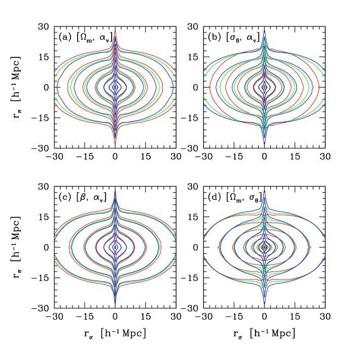
Figure 4: Contour plots of $\xi(r_{\sigma},r_{\pi})$ in the $r_{\sigma}-r_{\pi}$ plane, for the four sets of simulations listed in Table 2. The contours are separated by factors of two in $\xi(r_{\sigma},r_{\pi})$, with the outermost contours representing $\xi(r_{\sigma},r_{\pi})$$=2^{-4}$. (a) Models with $\Omega_{m}=0.3$, $\alpha_{v}=1$, and $\sigma_{8}=0.95$ (red), $\sigma_{8}=0.80$ (green), $\sigma_{8}=0.60$ (blue). (b) Models with $\sigma_{8}=0.8$, $\alpha_{v}=1$, and $\Omega_{m}=0.1$ (red), $\Omega_{m}=0.3$ (green), $\Omega_{m}=0.5$ (blue). (c) Models with $\beta\equiv\Omega_{m}^{0.6}/b_{g}=0.46$, $\alpha_{v}=1$, and $\sigma_{8}=0.95$ (red), $\sigma_{8}=0.80$ (green), $\sigma_{8}=0.60$ (blue). (d) Models with $\Omega_{m}=0.3$, $\sigma_{8}=0.8$, and $\alpha_{v}=0$ (red), $\alpha_{v}=0.8$ (green), $\alpha_{v}=1.2$ (blue).

Figure 5: Redshift-space correlation functions for the same models as in Figure 4, now plotted in the slice format, which allows easier identification of the small-scale distortion. In each panel, curves represent $r_{\sigma}=0.12$, 0.46, 2.54, and 14.2 $h^{-1}$Mpc from top to bottom. (a) Model with $\Omega_{m}=0.3$, $\alpha_{v}=1$, and $\sigma_{8}=0.95$ (dotted), $\sigma_{8}=0.80$ (solid), $\sigma_{8}=0.60$ (dashed). (b) Models with $\sigma_{8}=0.8$, $\alpha_{v}=1$, and $\Omega_{m}=0.1$ (dotted), $\Omega_{m}=0.3$ (solid), $\Omega_{m}=0.5$ (dashed). (c) Models with $\beta\equiv\Omega_{m}^{0.6}/b_{g}=0.46$, $\alpha_{v}=1$, and $\sigma_{8}=0.95$ (dotted), $\sigma_{8}=0.80$ (solid), and $\sigma_{8}=0.60$ (dashed). (d) Models with $\Omega_{m}=0.3$, $\sigma_{8}=0.8$, and $\alpha_{v}=0$ (dotted), $\alpha_{v}=0.8$ (solid), $\alpha_{v}=1.2$ (dashed). Errors are the run-to-run dispersion divided by $\sqrt{14}$ to calculate the error in the mean. Error bars are only plotted for the solid lines to avoid crowding.

Figure 6: Numerical results for the central model $(\Omega_{m}=0.3,\sigma_{8}=0.8,\alpha_{v}=1)$ compared to the best fit linear-exponential model. The solid lines are the numerical results and the dotted lines are the model. To fit the data, the exact value of $\beta$ was used, and the best fit dispersion $\sigma_{8}=418$ km s^-1 was found by $\chi^{2}$ minimization. Contour levels and $r_{\sigma}$ values are the same as those used in Figures 4 and 5.

3 Overview of $\xi(r_{\sigma},r_{\pi})$

Figure 4 encapsulates the dependence of the redshift-space correlation function, $\xi(r_{\sigma},r_{\pi})$, on position in the $(\Omega_{m},\sigma_{8},\alpha_{v})$ parameter space. Each panel shows contours of $\xi(r_{\sigma},r_{\pi})$, separated by factors of two, for a sequence of models in which two parameters or parameter combinations are held fixed and one is allowed to vary. Recall that these variations in cosmological parameters or velocity bias are carried out at fixed (or nearly fixed) real-space galaxy clustering, as shown in Figure 2. The green contours in each panel of Figure 4 show the central model with $\Omega_{m}=0.3$, $\sigma_{8}=0.8$, $\alpha_{v}=1.0$, $\alpha_{vc}=0$, and all models have $\Gamma=0.2$.

In panel (a), blue and red contours show models with $\sigma_{8}=0.6$ and 0.95, respectively, still with $\Omega_{m}=0.3$ and $\alpha_{v}=1$. As $\sigma_{8}$ increases, $\xi(r_{\sigma},r_{\pi})$ contours become more flattened because the amplitude of coherent flows increases with larger dark matter fluctuations. In terms of equation (1), higher $\sigma_{8}$ means a lower galaxy bias factor for fixed galaxy clustering amplitude, and thus a higher value of $\beta=\Omega_{m}^{0.6}/b_{g}$. In the FOG regime at small $r_{\sigma}$, contours of the three models are nearly degenerate at $r_{\pi}\leq 10$ $h^{-1}$Mpc. At these scales, most galaxy pairs are common members of intermediate mass halos, and the FOG distortion depends on the masses of those halos. The halo mass function is only weakly dependent on $\sigma_{8}$ at these intermediate masses, so the contours converge. However, a high-$\sigma_{8}$ model has more high mass halos with large virial velocity dispersions, so at large $r_{\pi}$ the contours extend further for higher $\sigma_{8}$.

Figure 4b shows a model sequence in which $\sigma_{8}=0.8$, $\alpha_{v}=1$, and $\Omega_{m}=0.1$ (red), 0.3 (green), and 0.5 (blue). The flattening of contours at large $r_{\sigma}$ and elongation at small $r_{\sigma}$ both increase with $\Omega_{m}$, since a higher density universe has larger amplitude coherent flows and more massive halos. While the large scale distortions have a similar qualitative dependence on $\sigma_{8}$ and $\Omega_{m}$, the FOG distortions show an important difference. Changing $\Omega_{m}$ shifts the halo mass function coherently at all masses, but changing $\sigma_{8}$ shifts the high and low ends of the mass function in opposite directions, with little change at intermediate masses. As a result, the FOG contours converge for the varying $\sigma_{8}$ sequence in panel (a) but not for the varying $\Omega_{m}$ sequence in panel (b).

In panel (c), we again vary $\sigma_{8}$ from 0.6 to 0.8 to 0.95, but for each value of $\sigma_{8}$ we choose the value of $\Omega_{m}$ that keeps the combination $\beta=\Omega_{m}^{0.6}/b_{g}$ constant. Note that $b_{g}$ is approximately proportional to $\sigma_{8}^{-1}$, so this sequence has approximately constant $\sigma_{8}\Omega_{m}^{0.6}$, but not exactly (see §4.4 for further discussion). Here the contours overlap almost perfectly on large and intermediate scales, and they are similar even in the FOG regime. While linear theory does not predict the form of $\xi(r_{\sigma},r_{\pi})$ accurately even on the largest scale shown (see Figure 6 below), it correctly predicts that the class of models with constant $\beta$ is nearly degenerate with respect to redshift-space distortions. The differences in the FOG regime, though difficult to see on this Figure, will nonetheless prove sufficient to distinguish models with the same $\beta$ but different $\sigma_{8}$.

In panel (d) we explore the effect of velocity bias. This sequence uses the central values of $\Omega_{m}=0.3$ and $\sigma_{8}=0.8$, (and thus has constant $\beta$), with $\alpha_{v}$ equal to 0, 0.8, and 1.2. For clarity, we omit the $\alpha_{v}=1$ model from the plot. The $\alpha_{v}=0$ model, which would represent measurements from a data set with perfect “FOG compression,” has elliptical contours at all scales, with no trace of the elongation at small $r_{\sigma}$. Since velocity bias is applied only within halos, these contours show that FOG distortions in $\xi(r_{\sigma},r_{\pi})$ arise entirely from halo internal velocity dispersions. At larger scales, the $\alpha_{v}=0$ model begins to coincide with the others when $r_{\sigma}\ga r_{\pi}$. The models with $\alpha_{v}=0.8$ and 1.2 diverge at approximately the same location, with higher $\alpha_{v}$ resulting in a stronger FOG effect. The small scale dispersion affects any global measure of the shape of $\xi(r_{\sigma},r_{\pi})$ contours, such as quadrupole-to-monopole ratios, but it has only a small effect at large $r_{\sigma}$ and $r_{\pi}$. We have also created two models, not shown in this figure, with no satellite velocity bias but with $\alpha_{vc}=0.2$ and 1. These models will be discussed in subsequent sections.

For the remainder of the paper, we will refer to these four model sequences by writing the parameters that are held constant in square brackets. Panel (a) plots the [$\Omega_{m},\alpha_{v}$] sequence, panel (b) plots the [$\sigma_{8},\alpha_{v}$] sequence, panel (c) plots the [$\beta,\alpha_{v}$] sequence, and panel (d) plots the [$\Omega_{m},\sigma_{8}$] sequence. The values of $\Omega_{m}$, $\sigma_{8}$, $\beta$, $\alpha_{v}$, and $\alpha_{vc}$ for these four model sequences are listed in Table 2.

Figure 5 plots the same results as Figure 4, but now in the form of Figure 3, showing slices at fixed values of $r_{\sigma}$. For each model, the top two curves trace out the FOG distortions at $r_{\sigma}\approx 0.12$ $h^{-1}$Mpc and $r_{\sigma}=0.46$ $h^{-1}$Mpc, allowing discrimination of models in the FOG regime that is difficult from the contour plots alone.

In panel (a), changes in $\sigma_{8}$ at fixed [$\Omega_{m},\alpha_{v}$] have only a small effect on the FOG distortions at $r_{\sigma}=0.12$ $h^{-1}$Mpc, though even these changes are significant relative to our statistical error bars, which are comparable to the line width. At $r_{\sigma}=14$ $h^{-1}$Mpc, the high-$\sigma_{8}$ model has higher $\xi(r_{\sigma},r_{\pi})$ at all $r_{\pi}$, but the large scale distortions are more difficult to discriminate in this representation compared to the contour plot (Fig. 4a).

Figure 7: The influence of HOD parameterization or halo concentration on predicted redshift-space distortions, when HOD parameters are chosen to yield the same real-space galaxy correlation function. All models assume $\Omega_{m}=0.3$, $\sigma_{8}=0.8$, $\alpha_{v}=1$. The top row compares results from our standard three-parameter HOD to the five-parameter HOD of Zheng et al. (2004). (a) Mean occupation functions $\langle N\rangle_{M}$ for the three-parameter HOD (solid line) and the five-parameter HOD (dotted line). The dashed curve is the satellite contribution to $\langle N\rangle_{M}$ for the five-parameter HOD. (b) $\xi(r_{\sigma},r_{\pi})$ contour plots for the three-parameter HOD (solid line) and the five-parameter HOD (dotted line, virtually indistinguishable). (c) Slices in $r_{\sigma}-r_{\pi}$ for the three-parameter HOD (solid lines) and five-parameter HOD (dotted lines). (d) — (f): Similar to (a) — (c), but dotted curves represent a model in which concentrations have been reduced by 30% and the HOD parameters (in the three-parameter model) have been adjusted to maintain the small-scale correlation function.

In the remaining panels, parameter changes have a marked effect on the FOG distortions at small $r_{\sigma}$. In particular, the models with constant [$\beta,\alpha_{v}$], which have nearly identical large scale distortions, show a $\sim 40\%$ change in $\xi(r_{\sigma},r_{\pi})$ at small $(r_{\sigma},r_{\pi})$ as $\sigma_{8}$ rises from 0.6 to 0.95 (Fig. 5c). While the separation of lines is not dramatic on a plot spanning five decades on the $y$-axis, differences of tens of percent should be easily measurable at these scales in the samples the size of the 2dFGRS and SDSS. Changing $\alpha_{v}$ from 0.8 to 1.2 has an effect of similar magnitude, though it differs in detailed form (Fig. 5d).

Figure 6 compares our numerical results for the central model $(\Omega_{m}=0.3,\sigma_{8}=0.8,\alpha_{v}=1)$ to the analytic, linear-exponential model of equation (2). We fix $\beta$ to the true value of 0.46 and vary $\sigma_{v}$ to minimize $\chi^{2}$ for all data at separations larger than 10 $h^{-1}$Mpc (we get similar $\sigma_{v}$ if we use data at all separations). The linear-exponential model describes the large scale distortions fairly well, though even here there are systematic differences between the numerical $\xi(r_{\sigma},r_{\pi})$ contours and the model fit. The model does a poor job of replicating the FOG distortions at large $r_{\pi}$, a failure that is evident in both the contour plots and the line plots. These deficiencies of the linear-exponential model can also be seen in its application to the 2dFGRS data by Peacock et  al. (2001, see their Figure 2). There, the measured distortions at small $r_{\sigma}$ clearly extend past the model predictions, even though the FOG effect has been smoothed relative to our plots here by the larger bin size. We can force the linear-exponential model to better match the FOG distortions by adopting a higher $\sigma_{v}$, but the fit at large scales is then severely degraded.

When analyzing observational data, we must infer the galaxy HOD by fitting parameterized models to the measured real-space clustering (e.g., the projected correlation function). We anticipate that redshift-space distortions will be insensitive to the adopted HOD parametrization so long as the model reproduces the observed real space correlation function. Figure 7 demonstrates the validity of this conjecture. We first populate the halos of our $\sigma_{8}=0.8$, $\Omega_{m}=0.3$ N-body simulations using a five-parameter HOD model fit to results of a hydrodynamic simulation (Zheng et al. 2004), in which the galaxy space density is $2.5\times 10^{-3}(h^{-1}{\rm Mpc})^{-3}$. This parameterization incorporates adjustable smooth cutoffs in the central and satellite galaxy mean occupation functions, and it can achieve an essentially perfect fit to the predictions of semi-analytic and numerical models of galaxy formation (Zheng et al. 2004). We then fit parameters of our restricted, three-parameter HOD model to reproduce the correlation function of the five-parameter model as closely as possible, obtaining agreement similar to that in Figure 2. Figure 7a shows the original and fitted mean occupation functions, and Figures 7b and 7c show $\xi(r_{\sigma},r_{\pi})$ for the two models, in the format of Figures 4 and 5, respectively. While the sharp cutoff model cannot represent the $\langle N\rangle_{M}$ of the input model exactly, it predicts essentially indistinguishable redshift-space distortions. The large scale distortions for both models are weaker than those in Figures 4 and 5 because our HOD parameters are matched to a strongly clustered galaxy sample with higher $b_{g}$ and consequently lower $\beta$.

As discussed in §2.2, our HOD models assume that satellite galaxies in halos have the same radial profile as the dark matter. If we change this assumption when fitting the observed correlation function, or if we make this assumption but it does not hold in the real universe, then we will derive slightly different HOD parameters, which in turn will change the redshift-space distortions. We test our sensitivity to the radial profile assumption by creating a model that matches $\xi_{R}(r)$ of our standard central model but uses satellite profile concentrations $30\%$ lower than those of the dark matter halos themselves. Figure 7d shows the mean occupation functions of the two models. The low concentration model has a lower $M_{1}$ to create more close one-halo pairs, and a lower $\alpha$ to prevent overpopulation of massive halos. Figures 7e and 7f show the redshift-space distortions of the two models. The large scale distortions of the two models are the same, apparent from both the contour plots and the line plots. The low concentration model has slightly weaker fingers-of-god because it has fewer galaxies in massive halos, but this difference is barely distinguishable in Figure 7f, and the difference in the quantitative measures of small scale distortion measures introduced in §5 is within our statistical errors. We conclude that departures from the standard radial profile by $\leq 30\%$ do not alter our results. Still larger changes might have noticeable effect, since the inferred HODs would predict different non-linear velocity fields, but substantial departures from theoretically predicted dark matter profiles can be detected observationally by measuring satellite galaxy profiles in groups and clusters.

4 Measures of Large-Scale Distortion and the Value of $\beta$

The blueprint for cosmological parameter estimation begins at large scales. At these scales, anisotropies are governed by the value of $\beta=\Omega_{m}^{0.6}/b_{g}$ (see Figure 4). The effects of velocity bias are limited and, we will show, straightforward to remove. Values of $b_{g}$ for our five values of $\sigma_{8}$ are listed in Table 1. We define galaxy bias factors by the ratio of the non-linear, real-space galaxy and matter correlation functions in the range $4\leq r\leq 12$ $h^{-1}$Mpc, $b_{g}^{2}\equiv\xi_{g}/\xi_{m}$, a choice that we discuss further in §4.4 below. Changing the range to $10\leq r\leq 25$ $h^{-1}$Mpc changes the values by $\la 1\%$. In characterizing distortions of the power spectrum or correlation function, we follow the track of Kaiser (1987), Hamilton (1992), and Cole et  al. (1994), using either the ratio of the angle-averaged redshift-space quantity to the real-space quantity, or the ratio of the quadrupole moment to the monopole in redshift space. The two methods applied to two statistics provide four measures of large scale distortions, illustrated by Figures 8–11 below.

4.1 The Power Spectrum

The angular dependence of the redshift-space galaxy power spectrum can be characterized as a sum of Legendre polynomials, denoted here as $L_{l}(\mu)$,

$$P_{Z}(k,\mu)=\sum_{l=0}^{\infty}P_{l}(k)L_{l}(\mu).$$ (5)

This equation can be inverted to determine each individual multipole by

$$P_{l}(k)=\frac{2l+1}{2}\int_{-1}^{+1}P_{Z}(k,\mu)L_{l}(\mu)d\mu.$$ (6)

Statistical symmetry of positive and negative peculiar velocities guarantees that odd multipoles vanish on average. In linear perturbation theory, only the $l=0,2$, and $4$ moments are non-zero. Equations (1) and (6) yield

$$P_{0}(k)=\left(1+\frac{2}{3}\beta+\frac{1}{5}\beta^{2}\right)P_{R}(k),$$ (7)

$$P_{2}(k)=\left(\frac{4}{3}\beta+\frac{4}{7}\beta^{2}\right)P_{R}(k),$$ (8)

for the monopole and the quadrupole, where $P_{R}(k)$ is the real-space power spectrum. In linear theory, the angle-averaged redshift-space power spectrum $P_{0}(k)$ is amplified over the real-space power spectrum by a constant factor, and the enhancement of fluctuations along the line of sight produces a positive quadrupole $P_{2}(k)$ with the same shape as $P_{R}(k)$. The ratio of the monopole to the real-space power spectrum, $P_{0/R}$, or the quadrupole-to-monopole ratio, $P_{2/0}$, are scale-independent functions of $\beta$:

$$P_{0/R}(k)\equiv\frac{P_{0}(k)}{P_{R}(k)}=1+\frac{2}{3}\beta+\frac{1}{5}\beta^{2}\,,$$ (9)

$$P_{2/0}(k)\equiv\frac{P_{2}(k)}{P_{0}(k)}=\frac{\frac{4}{3}\beta+\frac{4}{7}\beta^{2}}{1+\frac{2}{3}\beta+\frac{1}{5}\beta^{2}}\,\,.$$ (10)

However, non-linear effects, especially the velocity dispersions in collapsed or collapsing structures, suppress $P_{0}(k)$ at smallest scales and cause the quadrupole to actually reverse sign in the non-linear regime. In practice, the ratios $P_{0/R}$ and $P_{2/0}$ are monotonically decreasing functions of $k$, and equations (9) and (10) do not provide accurate estimates of $\beta$ at scales accessible to high-precision measurements. The use of the linear-exponential model (eq. 2) in place of pure linear theory (eq. 1) can greatly improve the accuracy of $\beta$ estimates, but it still does not remove biases entirely (Cole et al. 1995; Hatton & Cole 1999).

To calculate the redshift-space galaxy power spectra for our simulations, we use the same technique as Berlind, Narayanan, & Weinberg (2001). In the distant observer approximation, we take an axis of the box as the line of sight, wrap particles around the periodic boundary if their peculiar velocities shift them outside the box, and calculate $P_{Z}(k,\mu)$ by Fast Fourier Transform. We use a $200^{3}$ density mesh and treat each axis as an independent line of sight. The multipole moments are calculated by fitting the first three even terms in equation (6). We compute the average from 15 measurements (three projections of five simulations) and the errors by dividing the run-to-run dispersions by $\sqrt{14}$. Figures 8 and 9 show the results of this analysis for $P_{0/R}$ and $P_{2/0}$, respectively, as functions of wavelength $\lambda=2\pi/k$. Horizontal dotted lines represent the values of $P_{0/R}$ and $P_{2/0}$ predicted by linear theory (eqs. 9 and 10).

Figures 8a and 8b plot $P_{0/R}(k)$ for varying $\sigma_{8}$ and $\Omega_{m}$, respectively. At large $\lambda$, $P_{0/R}$ increases with increasing $\beta$. But all the curves drop rapidly at scales $\lambda\sim 30$ $h^{-1}$Mpc due to non-linearities. The difficulty in using linear theory to extract $\beta$ is easily seen; none of the models shows a clear asymptotic value of $P_{0/R}$. An estimate of the linear theory value might be possible for the lowest value of $\Omega_{m}$ or $\sigma_{8}$, but as either parameter increases the slope of the curve at large $\lambda$ becomes larger. At $\beta\ga 0.4$ the data never converge to the large-scale horizontal asymptote predicted by linear theory, even at the fundamental mode of the box.

For constant [$\beta,\alpha_{v}$], in panel (c), the curves are nearly identical within the error bars, especially at large scales. Thus, even though linear theory does not yield an accurate estimate of $\beta$, it predicts the scaling of $P_{0/R}$ with cosmological parameters almost perfectly, quantifying the visual impression of Figure 4c. In panel (d), the behavior of the $\alpha_{v}=0$ model demonstrates that random dispersion in virialized groups plays a dominant role on suppressing $P_{0/R}$. With the virial motions eliminated, the data for this model remain nearly constant over more than a decade in $\lambda$, with the other curves only meeting it at $\lambda\sim 100$ $h^{-1}$Mpc. A sufficiently effective FOG compression technique might therefore allow useful estimation of $\beta$ from linear theory and $P_{0/R}$.

The other velocity bias models begin to diverge from each other at $\lambda\sim 70$ $h^{-1}$Mpc, again demonstrating that cluster virial velocities affect redshift distortions well into what is normally considered the linear regime. If we allow central galaxies to move with respect to the halo center-of-mass with bias $\alpha_{vc}=0.2$, we find barely detectable changes (the line cannot be seen because it is directly beneath the line for the central model). We also plot the model with $\alpha_{vc}=1$, in which the central galaxy random velocities are the same magnitude as those of dark matter particles. At small scales, adding large central galaxy velocities has roughly the same effect as increasing the satellite velocity bias to $\alpha_{v}=1.2$, but the $\alpha_{vc}=1$ model converges with the central model somewhat faster.

Results for the quadrupole-to-monopole ratio are shown in Figure 9. The model dependence of $P_{2/0}$ is qualitatively similar to that of $P_{0/R}$, though the use of a higher order multipole leads to substantially larger statistical error. As with $P_{0/R}$, the $P_{2/0}$ curves only reach a large scale asymptote for the lowest values of $\beta$. Once again, however, linear theory correctly predicts that models with constant $\beta$ have the same large scale distortions. For the fixed [$\Omega_{m},\sigma_{8}$] model set in panel (d), the $\alpha_{v}=0$ model is consistent with linear theory at $\lambda>20$ $h^{-1}$Mpc. Increasing satellite velocity dispersions suppresses $P_{2/0}$ at steadily larger scales. Central galaxy velocities with $\alpha_{vc}=0.2$ produce almost no change, while the model with $\alpha_{vc}=1$ shows even stronger suppression than the satellite $\alpha_{v}=1.2$ model.

4.2 The Correlation Function

Since the power spectrum and correlation function are related by Fourier transformation, the linear theory approximation to $P_{Z}(k,\mu)$ also applies to $\xi(r_{\sigma},r_{\pi})$. Hamilton (1992) introduced the multipole approximation in configuration space, devising linear theory diagnostics of $\xi(r_{\sigma},r_{\pi})$ that parallel those in equations (9) and (10). The multipoles of the redshift space correlation function, $\xi_{l}(r)$, are calculated by the same inversion formula used in the Fourier domain,

$$\xi_{l}(r)=\frac{2l+1}{2}\int_{-1}^{+1}\xi(r_{\sigma},r_{\pi})L_{l}(\mu)d\mu,$$ (11)

where $r=\sqrt{r_{\sigma}^{2}+r_{\pi}^{2}}$ and $\mu=r_{\pi}/r$. The ratio of the monopole, $\xi_{0}(r)$, to the real-space correlation function, $\xi_{R}(r)$, exactly parallels equation (9),

$$\xi_{0/R}(r)\equiv\frac{\xi_{0}(r)}{\xi_{R}(r)}=1+\frac{2}{3}\beta+\frac{1}{5}\beta^{2}.$$ (12)

The quantity

$$Q_{\xi}(r)\equiv\frac{\xi_{2}(r)}{\xi_{0}(r)-\bar{\xi}_{0}(r)}=\frac{\frac{4}{3}\beta+\frac{4}{7}\beta^{2}}{1+\frac{2}{3}\beta+\frac{1}{5}\beta^{2}},$$ (13)

has the same asymptotic value as $P_{2/0}$ in linear theory (assumed for the second equality above). Here $\bar{\xi}_{0}(r)$ is the spherically averaged monopole,

$$\bar{\xi}_{0}(r)=\frac{3}{r^{3}}\int_{0}^{r}\xi_{0}(s)s^{2}ds.$$ (14)

We henceforth refer to $Q_{\xi}$ as the quadrupole of the redshift-space correlation function. To calculate $\xi_{0}(r)$ and $\xi_{2}(r)$, we bin galaxy pairs on a polar grid of logarithmic spacing in $r$ and linear spacing in angle, then perform the integral (11) numerically at each $r$.

Figure 10 shows the results for $\xi_{0/R}$, plotted as a linear function of $r$. In each panel, the curves reach an asymptotic value quickly, near $r=10$ $h^{-1}$Mpc. In most cases, the asymptote is above the dotted line representing the linear theory prediction. Despite this small systematic bias, which increases with increasing $\beta$, this diagnostic does not suffer from non-linear suppression of distortions at large scales; a fit to a constant value is straightforward. Another notable advantage of this diagnostic is that the effects of velocity bias (panel d) are almost negligible beyond $r=10$ $h^{-1}$Mpc. FOG compression ($\alpha_{v}=0$) removes the systematic offset between $\xi_{0/R}$ and the linear theory prediction at $r\sim 10-30$ $h^{-1}$Mpc. This result suggests that the offset is a consequence of FOGs transferring pairs from small separations in real space to large separations in redshift space.

Figure 11 plots $Q_{\xi}$ as a linear function of $r$. These curves resemble those of the power spectrum measures plotted as a function of $\log\lambda$. Models with low values of $\beta$ reach a horizontal asymptote at large $r$, while $Q_{\xi}$ for the high-$\beta$ models is still increasing at the largest separation. All the curves are under the predicted linear theory values, in contrast to the results for $\xi_{0/R}$. Figure 11d shows that small scale dispersions are the main effect suppressing $Q_{\xi}$; with $\alpha_{v}=0$, $Q_{\xi}$ tracks the linear theory prediction down to $r=10$$h^{-1}$Mpc. Increasing satellite or central galaxy velocity dispersions drives the non-linear suppression of $Q_{\xi}$ to larger scales.

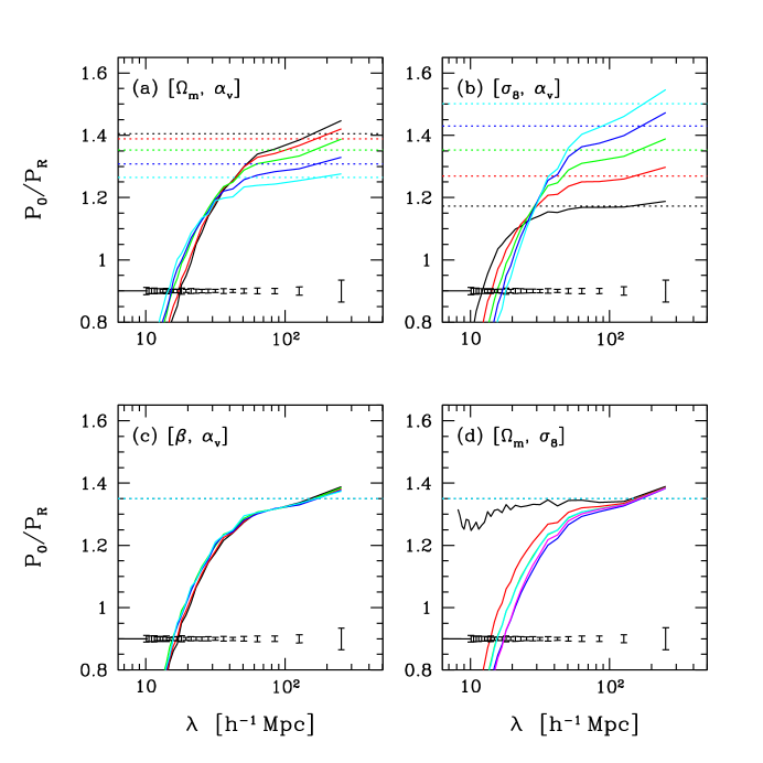
Figure 8: Monopole-to-real space ratio of the power spectrum, $P_{0}/P_{R}$, as a function of wavelength, up to the fundamental mode of the 253 $h^{-1}$Mpc box. The dotted lines represent the linear theory prediction for each model for this measure. The error bars plotted at the bottom of each panel are errors in the mean for the central model, which are generally representative of the error bars for the rest of the models in each set. Models run from $\sigma_{8}=0.95$ (black) to $\sigma_{8}=0.6$ (cyan) in panel (a), from $\Omega_{m}=0.1$ (black) to $\Omega_{m}=0.5$ (cyan) in panel (b), and from $\sigma_{8}=0.95$ (black) to $\sigma_{8}=0.6$ (cyan) in panel (c), with the order of the colors being black, red, green, blue, cyan. In panel (d), models are $\alpha_{v}=0$ (black), $\alpha_{v}=0.8$ (red), $\alpha_{v}=1.0$ (green), $\alpha_{v}=1.2$ (blue), and $\alpha_{vc}=0.2$ (cyan, barely separable from green), and $\alpha_{vc}=1$ (magenta).

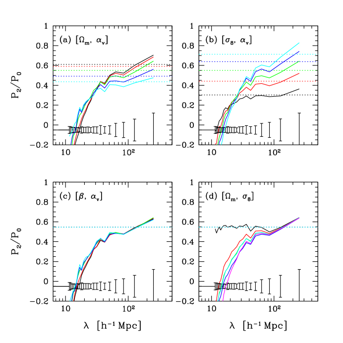
Figure 9: Quadrupole-to-monopole ratio of the redshift space power spectrum, $P_{2}/P_{0}$, as a function of wavelength, up to the fundamental mode of the 253 $h^{-1}$Mpc box. The dotted lines and error bars are as in Figure 8. Models run from $\sigma_{8}=0.95$ (black) to $\sigma_{8}=0.6$ (cyan) in panel (a), from $\Omega_{m}=0.1$ (black) to $\Omega_{m}=0.5$ (cyan) in panel (b), from $\sigma_{8}=0.95$ (black) to $\sigma_{8}=0.6$ (cyan) in panel (c), with the order of the colors being black, red, green, blue, cyan. In panel (d), models are $\alpha_{v}=0$ (black), $\alpha_{v}=0.8$ (red), $\alpha_{v}=1.0$ (green), $\alpha_{v}=1.2$ (blue), and $\alpha_{vc}=0.2$ (cyan, barely separable from green), and $\alpha_{vc}=1$ (magenta).

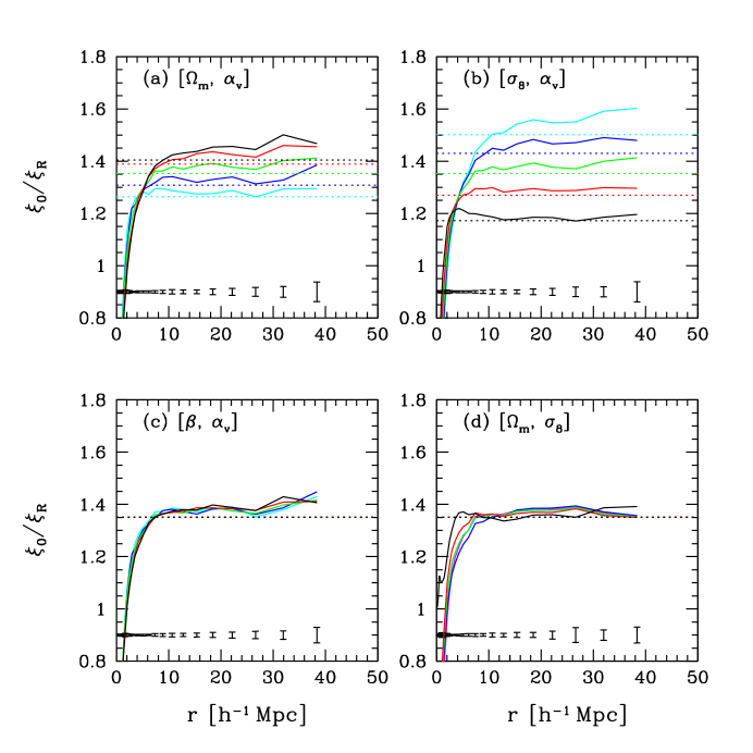
Figure 10: Ratio of the monopole of the redshift-space correlation function to the real-space correlation function, $\xi_{0/R}$, as a function of separation $r$. The dotted lines and error bars are as in Figure 8. Models run from $\sigma_{8}=0.95$ (black) to $\sigma_{8}=0.6$ (cyan) in panel (a), from $\Omega_{m}=0.1$ (black) to $\Omega_{m}=0.5$ (cyan) in panel (b), from $\sigma_{8}=0.95$ (black) to $\sigma_{8}=0.6$ (cyan) in panel (c), with the order of the colors being black, red, green, blue, cyan. In panel (d), models are $\alpha_{v}=0$ (black), $\alpha_{v}=0.8$ (red), $\alpha_{v}=1.0$ (green), $\alpha_{v}=1.2$ (blue), and $\alpha_{vc}=0.2$ (cyan, barely separable from green), and $\alpha_{vc}=1$ (magenta).

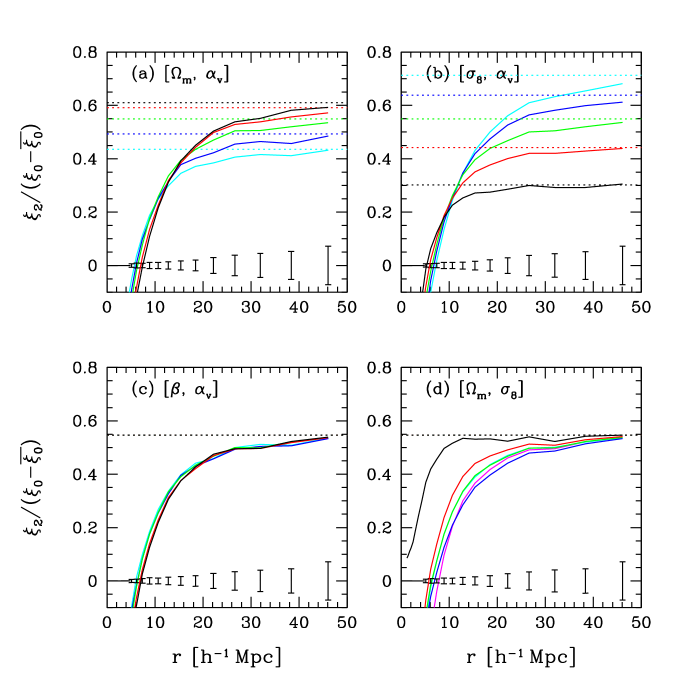
Figure 11: Quadrupole moment of the correlation function, $Q_{\xi}=\xi_{2}/(\xi_{0}-\bar{\xi}_{0})$, as a function of separation. The dotted lines and error bars are as in Figure 8. Models run from $\sigma_{8}=0.95$ (black) to $\sigma_{8}=0.6$ (cyan) in panel (a), from $\Omega_{m}=0.1$ (black) to $\Omega_{m}=0.5$ (cyan) in panel (b), from $\sigma_{8}=0.95$ (black) to $\sigma_{8}=0.6$ (cyan) in panel (c), with the order of the colors being black, red, green, blue, cyan. In panel (d), models are $\alpha_{v}=0$ (black), $\alpha_{v}=0.8$ (red), $\alpha_{v}=1.0$ (green), $\alpha_{v}=1.2$ (blue), and $\alpha_{vc}=0.2$ (cyan, barely separable from green), and $\alpha_{vc}=1$ (magenta).

4.3 Estimating $\beta$

The $\alpha_{v}=0$ curves in Figures 8d, 9d, 10d, and 11d show that $\beta$ can be estimated fairly accurately using linear theory if FOG distortions are removed by suppressing velocity dispersions in virialized halos. However, these curves represent a case in which FOG compression is perfect, with halos identified in real space from the densely sampled dark matter distribution. Any realistic scheme must operate on the sparsely sampled galaxy distribution in redshift space, and it will suffer from incompleteness and contamination of the halo catalog and incorrect assignments of galaxies to halos. The impact of these imperfections on $\beta$ estimates must be evaluated in the context of a specific group identification scheme applied to a survey with specified depth and geometry, and we will not consider the FOG compression approach further in this paper. Instead, we will use our numerical results to devise fitting procedures that estimate $\beta$ and a characteristic non-linear scale from measurements of $P_{2/0}(k)$, $P_{0/R}(k)$, $\xi_{0/R}(r)$, and $Q_{\xi}(r)$. In the remainder of the paper, we use the notation $\beta_{\rm fit}$ to represent a value of $\beta$ estimated by one of these fitting procedures, and use $\beta$ to represent the true model values of $\Omega_{m}^{0.6}/b_{g}$. The forms of our fitting functions are arbitrary, motivated by efficacy rather than theoretical arguments, but they all encode the general behavior of linear distortions at large scales suppressed or reversed by non-linear effects at small scales.

For the quadrupole-to-monopole ratio of the power spectrum, our procedure is similar to that proposed by Hatton & Cole (1999; hereafter HC99), who suggest the fitting formula

$$P_{2/0}(\lambda)=P_{2/0}^{\rm lin}\left[1-(\lambda/\lambda_{0})^{-1.22}\right].$$ (15)

Here $P_{2/0}^{\rm lin}$ is the linear theory quadrupole distortion, related to $\beta$ by equation (10), and $\lambda_{0}$ is the non-linear scale at which the quadrupole passes through zero. We make two changes to the HC99 procedure, which, in our experiments, improve the accuracy and robustness of the $\beta$ estimates. First, we calculate $\lambda_{0}$ by fitting a straight line to the six data points surrounding $P_{2/0}=0$, instead of leaving it as a fitting parameter in the global fit. Second, we modify equation (15) to

$$P_{2/0}(\lambda)=P_{2/0}^{\rm lin}\left[1-\left(\frac{\lambda}{\lambda_{0}}\right)^{-1.55/(0.45+P_{2/0}^{\rm lin})}\right].$$ (16)

We determine the fitting parameter $P_{2/0}^{\rm lin}$ by minimizing $\chi^{2}$ for all data points with $\lambda\geq\lambda_{0}$, ignoring any covariance of errors, and we then solve for $\beta_{\rm fit}$ using equation (10). Since $P_{2/0}^{\rm lin}$ varies around $\sim 0.55$, the exponent in equation (16) is similar to that in HC99’s formula, but including a dependence on $P_{2/0}^{\rm lin}$ captures the behavior seen in Figure 9, where the $P_{2/0}$ curves for higher $\beta$ models flatten toward their asymptotic values at larger scales.

Figure 12: The relative errors in $\beta_{\rm fit}$ obtained from the fitting functions, for models with $\Gamma=0.2$ (left) and $\Gamma=0.12$ (right). In each panel, the solid lines represent zero error, while the dotted lines are $\pm 10\%$ error. The four different point types correspond to the four model sets in Table 2: constant [$\Omega_{m},\alpha_{v}$] (squares), constant [$\sigma_{8},\alpha_{v}$] (triangles), constant [$\beta,\alpha_{v}$] (stars), constant [$\Omega_{m},\sigma_{8}$] (hexagons). The $\alpha_{v}=0$ model is not shown. The $\alpha_{vc}=1$ model is plotted with a solid circle (left panels only). The bottom panels show, with an expanded vertical scale, the systematic errors of the linear-exponential model and the HC99 fitting method.

We use a similar procedure to estimate $\beta$ from $P_{0/R}(\lambda)$. Here we define the non-linear scale $\lambda_{1}$ as the wavelength at which $P_{Z}=P_{0}$, and we determine it by fitting a straight line to the six data points around $P_{0/R}=1$. We fit the functional form

$$P_{0/R}(\lambda)=(P_{0/R}^{\rm lin}-1)\left[1-\left(\frac{\lambda}{\lambda_{1}}\right)^{-1.57/(0.50+\beta_{\rm fit})}\right]+1,$$ (17)

where $\beta_{\rm fit}$ and $P_{0/R}^{\rm lin}$ are related by equation (9). We estimate $\beta_{\rm fit}$ by minimizing $\chi^{2}$ for all data points with $\lambda\geq\lambda_{1}$. As with equation (16), the form of the exponent captures our numerical finding that higher $\beta$ models approach asymptotic behavior more slowly. In this case, we found that using $\beta_{\rm fit}$ rather than $P_{0/R}^{\rm lin}$ in the denominator of the exponent produced more accurate results.

For $Q_{\xi}$, we adopt the fitting function

$$Q_{\xi}(r)=Q_{\xi}^{\rm lin}\left[1-\left(\frac{1.45}{\beta_{\rm fit}}\right)^{0.75(1-r/R_{0})}\right],$$ (18)

where once again $Q_{\xi}^{\rm lin}$ is the free parameter and its relation to $\beta_{\rm fit}$ is defined in equation (13). The parameter $R_{0}$ is the scale at which $\xi_{2}(r)=0$. Since the data for $Q_{\xi}$ are much smoother than those for the power spectrum diagnostics, it is sufficient to fix $R_{0}$ by simple interpolation between the two points surrounding $Q_{\xi}=0$. We determine $\beta_{\rm fit}$ by minimizing $\chi^{2}$ for data points with $r\geq R_{0}$.

For $\xi_{0/R}$, we find that the most effective method to estimate $\beta$ is simply to fit a straight line to all data above $r=10$ $h^{-1}$Mpc, and calculate $\beta_{\rm fit}$ from linear theory. A minimum scale below 10 $h^{-1}$Mpc allows non-linearities to affect the fit, while a larger minimum scale reduces the precision because the error bars increase monotonically with $r$.

Figure 12 presents the main quantitative results of this section, showing the fractional error $\epsilon\equiv(\beta_{\rm fit}-\beta)/\beta$ of the $\beta$ estimates from $P_{2/0}$, $P_{0/R}$, $Q_{\xi}$, and $\xi_{0/R}$, using the fitting procedures described above. For the left hand panels, we fit the curves shown in Figures (8)—(11), which are averaged over three projections of the five $\Gamma=0.2$ simulations. Right hand panels show results of the same procedures for the $\Gamma=0.12$ simulations.

Squares represent the fixed [$\sigma_{8},\alpha_{v}$] model sequence, with the $\Omega_{m}$ range $0.1-0.5$ producing $\beta$ values from 0.24 to 0.63 (see Table 2). The fixed [$\Omega_{m},\alpha_{v}$] sequence, shown by the triangles, spans a narrower range of $0.36\leq\beta\leq 0.53$, since we limit $\sigma_{8}$ to the range $0.6-0.95$. Five-point stars represent [$\beta,\alpha_{v}$] models, which all have $\beta=0.46$ by construction. Hexagons represent the $\alpha_{v}=0.8$ and $\alpha_{v}=1.2$ models from the fixed [$\Omega_{m},\sigma_{8}$] sequence. The $\alpha_{v}=1.0$ model is the same as the central model by definition, and the model with $\alpha_{vc}=0.2$ is indistinguishable from it in practice, so we omit it from the plot. The $\alpha_{vc}=1$ model is shown with the small filled circle (left panels only). We do not show results for the FOG compression model because our fitting procedures do not apply to it.

Table 3: Errors in $\beta_{\rm fit}$

	$\Gamma=0.2$		$\Gamma=0.12$
Method	$\langle\epsilon^{2}\rangle^{1/2}$ [%]	$\langle\epsilon\rangle$ [%]	$\langle\epsilon^{2}\rangle^{1/2}$ [%]	$\langle\epsilon\rangle$ [%]
$P_{2/0}$	4.4	1.9	4.2	1.9
$P_{0/R}$	1.3	0.6	1.8	-0.7
$Q_{\xi}$	4.3	0.7	3.5	1.7
$\xi_{0/R}$	6.1	5.9	11.3	10.9
Lin+Exp	9.4	4.2	18.4	14.6
HC99	14.9	14.0	17.3	16.5

For the fixed [$\sigma_{8},\alpha_{v}$] sequence, we calculate the statistical uncertainty in our estimate of the fractional error $\epsilon$ by separately fitting the five simulations in turn, then dividing the dispersion of the $\beta_{\rm fit}$ values by $\sqrt{5-1}=2$ to obtain the uncertainty in the mean. These uncertainties are shown by error bars on the squares in Figure 12. In many but not all cases, our measurement of the bias in $\beta_{\rm fit}$ for a given model is consistent with zero, or only marginally inconsistent with it. However, even when the offsets from zero are within the error bars, the trend with model parameters along a sequence may be significant, since all of our models are based on the same set of simulations. The total volume of our simulations is $5\times(253$$h^{-1}$Mpc$)^{3}$, equivalent to that of redshift survey covering 8000 square degrees to a limiting depth of 460 $h^{-1}$Mpc. Since the three orthogonal projections sample different random orientations of the large scale structures in each simulation, the effective volume is somewhat larger, though the increase is not a full factor of three because real-space structures are the same in each projection. The error bars in Figure 12 are therefore similar in magnitude to the statistical error expected from the full SDSS redshift survey, which will cover 8000 square degrees with a median galaxy redshift $\sim 0.1$ (Strauss et al. 2002).

Table 3 summarizes the performance of the four $\beta$-estimators, listing the mean and rms value of the fractional errors plotted in Figure 12. Note, however, that the numbers depend on the particular set of models we have chosen, so they are only a rough indicator. For $\xi_{0/R}$, our procedure of fitting a straight line to the measurements above 10 $h^{-1}$Mpc gives a precise but not accurate value of $\beta_{\rm fit}$, as seen earlier in Figure 10. The mean offset is 5.9% for $\Gamma=0.2$ and 10.9% for $\Gamma=0.12$. The rms values of $\epsilon$ are only slightly larger, consistent with the small scatter around the the mean offset seen in Figure 12, though for $\Gamma=0.12$ there is a weak but clearly significant trend of $\epsilon$ with $\beta$. Increasing the minimum fit radius above 10 $h^{-1}$Mpc reduces the correlation but does not eliminate the higher mean error.

The $P_{0/R}$ fits yield accurate $\beta$ estimates, with mean errors of less than $1\%$ that are within the statistical uncertainty of our calculations. The rms errors are only $1.3\%$ and $1.8\%$ for $\Gamma=0.2$ and $\Gamma=0.12$, respectively. Velocity bias does have a noticeable effect on the $P_{0/R}$ estimator, with $\pm 20\%$ changes in $\alpha_{v}$ producing $\mp 2.4\%$ changes in $\beta_{\rm fit}$.

Errors for the quadrupole estimators $P_{2/0}$ and $Q_{\xi}$ are larger, in part because of our larger statistical uncertainties, but also because of stronger variation with model parameters. Velocity bias has a significant impact on $P_{2/0}$, with $\pm 20\%$ changes in $\alpha_{v}$ producing $\mp 9\%$ changes in $\beta_{\rm fit}$ for $\Gamma=0.2$. For $Q_{\xi}$ the effect is smaller, $\mp 5.5\%$. The slope traced by the triangular points shows that the bias of the $Q_{\xi}$ estimator changes steadily with $\sigma_{8}$, from $-6\%$ at $\sigma_{8}=0.6$ to $+8\%$ at $\sigma_{8}=0.95$ for $\Gamma=0.2$. A similar trend with $\sigma_{8}$ appears in the constant-$\beta$ sequence.

For comparison, the lower panels of Figure 12 show the results of applying the HC99 and linear-exponential models to our simulation results. The HC99 procedure is applied to $P_{2/0}$ measurements with $P_{2}(k)\geq 0$, and we implemented the linear-exponential model by minimizing $\chi^{2}$ with respect to $\xi(r_{\sigma},r_{\pi})$ for all data with $r\geq 5$ $h^{-1}$Mpc. Note the larger vertical scale on these panels. The HC99 simulations emphasized values of $\beta\ga 0.6$, and for $\beta\ga 0.5$ we also find it to be fairly accurate, with a bias $\sim 10\%$. However, for lower $\beta$ values the HC99 procedure substantially overestimates the true $\beta$, and our modification defined by equation (16) is a major improvement.

The linear-exponential model performs reasonably well for $\Gamma=0.2$, but there is a steady trend from positive bias at low $\beta$ to negative bias at high $\beta$, and the rms error of $9.4\%$ is substantially larger than for any of our estimators. Increasing the minimum fitting scale from 5 $h^{-1}$Mpc to 10 $h^{-1}$Mpc makes little difference. For $\Gamma=0.12$ the linear-exponential model breaks down more seriously, overestimating $\beta$ by up to 40%, and showing strong correlation of the $\beta_{\rm fit}$ error with $\beta$ and with $\sigma_{8}$.

By determining non-linear scales directly from the data, our $\beta$-fitting procedures avoid any explicit dependence on $\sigma_{8}$, $\Omega_{m}$, or $\alpha_{v}$. Or course, for known values of $\sigma_{8}$ or $\alpha_{v}$, one could use Figure 12 to remove the bias of the estimator, further improving its accuracy. Our fitting formulas (16)—(18) are obtained empirically, with only a qualitative relation to a full physical model. However, they successfully describe models with a wide range of physical parameters, and we will show in §4.5 below that the non-linear scales in these fits depend on $\sigma_{8}$, $\Omega_{m}$, and $\alpha_{v}$ in physically sensible ways.

The estimates based on redshift-space to real-space ratios, $P_{0/R}$ and $\xi_{0/R}$, perform more robustly than those involving quadrupole moments, once the linear theory estimate from $\xi_{0/R}$ is corrected for systematic bias. Furthermore, the monopole components $P_{0}(k)$ and $\xi_{0}(r)$ can be measured with higher precision than the quadrupoles $P_{2}(k)$ and $\xi_{2}(r)$, for a data set of fixed size. However, we have not addressed the problem of determining the real-space quantities $P_{R}(k)$ and $\xi_{R}(r)$. Hamilton et al. (2000) propose methods for recovering the former, by combining the monopole, quadrupole, and hexadecapole on large scales, and using the power in modes transverse to the line of sight on small scales. For $\xi_{R}(r)$, one can invert the projected correlation function $w_{p}(r_{p})$ (see Davis & Peebles 1983; Zehavi et al. 2004b). Alternatively, having fit $w_{p}(r_{p})$ with an HOD model, one can take the three-dimensional correlation function of that model to represent $\xi_{R}(r)$. It is possible that estimating $P_{R}(k)$ or $\xi_{R}(r)$ in these ways will degrade the performance of the redshift-to-real space estimators, introducing systematic errors or larger statistical errors. We leave that question to future work that involves mock catalogs tailored to specific data sets.

4.4 From $\beta$ and $\Omega_{m}$ to $\sigma_{8}$

With sufficiently good observational data, the procedures described in §4.3 can provide estimates of $\beta\equiv\Omega_{m}^{0.6}/b_{g}$ that are accurate to a few percent or better. For a specified value of $\Omega_{m}$, this estimate in turn yields an estimate of $b_{g}$. However, for cosmological purposes we are less interested in $b_{g}$ per se than in the dark matter fluctuation amplitude $\sigma_{8}$. In this paper we define $b_{g}$ to be the mean value of $[\xi_{g}(r)/\xi_{m}(r)]^{1/2}$ over the range 4 $h^{-1}$Mpc $\leq r\leq$ 12 $h^{-1}$Mpc, where the average is inverse variance weighted and $\xi_{m}(r)$ is the non-linear correlation function of the simulation dark matter particles. The value of $b_{g}$ is insensitive to increases in the inner or outer cutoff on the averaging regions, though it drops if the minimum radius is pushed much below 4 $h^{-1}$Mpc. For example, changing the range to 10 $h^{-1}$Mpc $\leq r\leq$ 25 $h^{-1}$Mpc, changes $b_{g}$ of the central model from 1.041 to 1.026, the largest change of the five models.

Figure 13: Comparison of bias definitions. Curves show the square root of the ratio of the non-linear galaxy and linear matter power spectra, for the five $\sigma_{8}$ values as indicated. Error bars shown for the $\sigma_{8}=0.95$ model are the error in the mean from five realizations. Thin lines are the value of $b_{g}$ measured from the correlation function ratio and used in our definition of $\beta$.

The standard analytic approximation for the large-scale bias factor,

$$b_{g}=\frac{1}{\bar{n}_{g}}\,\int_{0}^{\infty}\,b_{h}(M)\,\langle N\rangle_{M}\,\frac{dn}{dM}\,dM,$$ (19)

describes our numerical results for $b_{g}$ with an rms error of 0.4% for $\Gamma=0.2$ and 0.6% for $\Gamma=0.12$, if we use the halo bias formula $b_{h}(M)$ of Tinker et al. (2004) and the halo mass function $dn/dM$ of Jenkins et al. (2001). The bias $b_{g}$ is a monotonically decreasing function of $\sigma_{8}$, since we match the same galaxy correlation function by construction. The most robust way to convert a value of $\beta_{\rm fit}$ to a value of $\sigma_{8}$ (for a specified $\Omega_{m}$) is to consider a sequence of models of increasing $\sigma_{8}$, carry out HOD fits to match the observed projected correlation function $w_{p}(r_{p})$ in each case, compute $b_{g}$ from $\langle N\rangle_{M}$ using equation (19), and pick the value of $\sigma_{8}$ for which $\Omega_{m}^{0.6}/b_{g}=\beta_{\rm fit}$.

By definition, $\sigma_{8}$ is given by an integral over the linear theory dark matter power spectrum $P_{\rm lin}(k)$. In the linear approximation, where $b_{g}^{2}=P_{g}(k)/P_{\rm lin}(k)$, one can use an estimated $b_{g}$ and the measured galaxy power spectrum $P_{g}(k)$ to normalize $P_{\rm lin}(k)$ and thus compute $\sigma_{8}$. Figure 13 compares our definition of $b_{g}$ (horizontal lines) to the power spectrum ratios $[P_{g}(k)/P_{\rm lin}(k)]^{1/2}$ of the $\Gamma=0.2$ simulations. For all five values of $\sigma_{8}$, the power spectrum ratios are consistent with a constant asymptotic value at large scales, and this asymptotic value is consistent with the value of $b_{g}$ defined from the correlation function ratio. However, even with our $360^{3}$ simulations, we cannot make this comparison at a precision better than a few percent because there are relatively few Fourier modes in the asymptotic regime. Furthermore, the power spectrum ratios lie slightly above $b_{g}$ for $\sigma_{8}=0.6$ and slightly below for $\sigma_{8}=0.95$, with a steady trend in between. The same trend appears in Table 1, where the product $\sigma_{8}b_{g}$ rises from 0.81 to 0.88 as $\sigma_{8}$ grows from 0.6 to 0.95. Thus, simply normalizing $P_{\rm lin}(k)$ by $P_{g}(k)/b_{g}^{2}$ would not accurately describe our results at the few percent level. The trend of $\sigma_{8}b_{g}$ arises because we set our HOD parameters by fitting the galaxy correlation function in the linear and non-linear regime; at the few percent level, our large-scale galaxy correlation function is higher for high $\sigma_{8}$ (see Figure 2). If we forced a perfect match of the galaxy correlation function at large scales, then $\sigma_{8}b_{g}$ would be constant, but we could no longer match $\xi_{R}(r)$ as well at small scales, at least with our three-parameter HOD.

The passage from $\beta$ and $\Omega_{m}$ to $\sigma_{8}$ would be easy if we defined the galaxy bias $b_{g}=b_{8}\equiv\sigma_{8,g}/\sigma_{8}$, where $\sigma_{8,g}$ is the (non-linear, shot noise subtracted) rms galaxy count fluctuation in 8 $h^{-1}$Mpc spheres. In this case, one could simply divide $\beta_{\rm fit}$ by $\Omega_{m}^{0.6}$ and multiply by the measured $\sigma_{8,g}$ to obtain $\sigma_{8}$. We have tried to develop procedures like those in §4.3 to estimate $\beta_{8}\equiv\Omega_{m}^{0.6}/b_{8}$. However, once we tune the estimation formulas to the $\Gamma=0.2$ simulations, they do not provide accurate results for $\Gamma=0.12$, in contrast to our procedures for $\beta$, which give accurate results for both power spectrum shapes. An 8 $h^{-1}$Mpc top-hat does not suppress non-linear clustering enough for the bias factor $b_{8}$ to approximate bias in the linear regime (as also noted by HC99).

In Paper II, we develop an analytic approach that circumvents the complication of mapping $\beta$ into the $\sigma_{8}-\Omega_{m}^{0.6}$ parameter space, as the fitting parameters are $(\Omega_{m},\sigma_{8},\alpha_{v})$, without reference to $\beta$.

4.5 Length Scales in Large-Scale Distortions

Figure 14: Influence of cosmological parameters on the non-linear length scales of the large-scale distortion measures. (a) The wavelength $\lambda_{1}$ at which $P_{0}/P_{R}=1$ is plotted against $\beta\sigma_{8}^{1/2}\alpha_{v}^{2}$. Large and small points show the $\Gamma=0.2$ and $\Gamma=0.12$ results, respectively, with point types corresponding to model sequences as indicated in the legend. (b) — (d) Non-linear length scales for the other three large-scale measures, plotted against the combinations of $\beta$, $\sigma_{8}$, and $\alpha_{v}$ that produce the least scatter, for $\Gamma=0.2$. Dotted lines show least squares fits to the data points.

The distortions in redshift-to-real space and quadrupole-to-monopole ratios in Figures 8 and 11 are driven mainly by galaxy velocity dispersions on small and intermediate scales, which drive down the redshift-space correlation amplitude and reverse the sign of quadrupole distortions. The non-linear length scales in equations (9), (10), and (13), and the radius $R_{1}$ at which $\xi_{0}=\xi_{R}$, therefore encode information about the parameters $\Omega_{m}$, $\sigma_{8}$, and $\alpha_{v}$, as an increase in any of these variables increases the galaxy velocity dispersion. The dependence of the galaxy velocity dispersion on $\Omega_{m}$ is straightforward: at fixed $\sigma_{8}$, the large-scale velocity field follows the linear theory scaling $\Omega_{m}^{0.6}$, and the virial velocities of halos of fixed abundance scale as $\Omega_{m}^{1/2}$ (ignoring the small dependence of halo concentration on $\Omega_{m}$). These two effects appear at different scales, but we find that the pairwise galaxy velocity dispersion scales roughly as $\Omega_{m}^{0.55}$ in our simulations at all separations. For $\sigma_{8}$ and $\alpha_{v}$, the situation is more complicated. Velocity bias is most influential at small scales, where the galaxy pairs come from within one halo. At larger scales, a significant fraction of pairs involve the central galaxies of low-mass halos, and are thus not affected by satellite velocity bias. Inspection of our numerical results suggests that at large separations the pairwise dispersion scales as $\alpha_{v}^{1/2}$. The power spectrum normalization affects the galaxy velocity dispersion in two ways: at linear scales the halo velocity dispersion increases linearly with $\sigma_{8}$, while the internal velocity dispersions of halos hosting multiple galaxies increase with $\sigma_{8}$ because of the higher halo masses.

Inspection of the analytic solution for $P_{0/R}$ in the linear-exponential model (see Cole et al. 1995, §2.1) implies that the non-linear scale $\lambda_{1}$ where $P_{0/R}=1$ should scale linearly with the velocity dispersion $\sigma_{v}$ at fixed $\beta$ and approximately as $\beta^{-1/2}$ at fixed $\sigma_{v}$. With the scalings $\sigma_{v}\propto\Omega_{m}^{0.55}\alpha_{v}\sigma_{8}$ discussed above, we obtain

$$\lambda_{1}\propto\beta^{-1/2}\sigma_{v}\propto\Omega_{m}^{0.25}\sigma_{8}^{0.5}\alpha_{v},$$ (20)

where the last relation uses $\beta\propto\sigma_{8}\Omega_{m}^{0.6}$.

The left-hand panel of Figure 14 plots $\lambda_{1}$ against $\beta\sigma_{8}^{1/2}\alpha_{v}^{2}$, a combination of parameters chosen by trial and error to yield minimal scatter. The numerical data form a tight power-law for the $\Gamma=0.2$ models. The statistical errors derived from the run-to-run dispersion are of order the point size, and the fit has a $\chi^{2}$ per degree of freedom of 8.9, indicating that most of the model-to-model scatter is physical in origin. The data for the $\Gamma=0.12$ models follow the same slope, but the amplitude of the relation is 5% higher, and there is more scatter. The dotted line plotted in the panel is a least squares fit to the $\Gamma=0.2$ data. The slope is $\sim 0.36$, making a scaling of $\lambda_{1}=26.3\,\Omega_{m}^{0.22}\sigma_{8}^{0.54}\alpha_{v}^{0.72}$ $h^{-1}$Mpc. Given the approximate nature of the arguments behind equation (20), the agreement with the numerically derived scaling is quite good. The lower index on $\alpha_{v}$ in the numerical results arises because the scale $\lambda_{1}\sim 10$ $h^{-1}$Mpc is outside the one-halo regime where $\sigma_{v}\propto\alpha_{v}$ but not fully in the large scale regime where $\sigma_{v}\propto\alpha_{v}^{1/2}$.

The remaining panels of Figure 14 plot the other non-linear length scales against a combination of parameters chosen by trial and error to produce minimum scatter. For the central model, the $P_{2/0}$ zero-crossing $\lambda_{0}$ is slightly smaller than $\lambda_{1}$, $\lambda_{0}$ is $\sim 2$ times the $Q_{\xi}$ zero-crossing $R_{0}$, and $R_{0}$ is $\sim 3$ times the scale $R_{1}$ at which $\xi_{0/R}=1$. Dotted lines show best-fit power-law relations, $\lambda_{0}=20.7\,(\beta\sigma_{8}\alpha_{v}^{2})^{0.28}$, $R_{0}=8.7(\beta\sigma_{8}\alpha_{v}^{2})^{0.30}$, $R_{1}=2.9\,(\beta\sigma_{8}^{1/2}\alpha_{v})^{0.50}$. Scatter for the quadrupole length scales is consistent with the statistical errors (see panel b), which are larger for these measurements.

In principle, these non-linear length scales can help determine cosmological parameters by adding another observable quantity to break degeneracies in our three-dimensional parameter space. For example, once $\beta$ is fixed by the large-scale distortions, the measurement of $\lambda_{1}$ constrains the parameter combination $\sigma_{8}^{0.18}\alpha_{v}^{0.72}$. Since the different length scales have different parameter dependencies, once can use combinations to isolate $\alpha_{v}$ and $\sigma_{8}$. For example, the best-fit power laws imply

$$\alpha_{v}=\left(\frac{\lambda_{1}}{26.9\,h^{-1}\mbox{Mpc}}\right)^{2.78}\left(\frac{R_{1}}{2.92\,h^{-1}\mbox{Mpc}}\right)^{-2.00}.$$ (21)

The models with no velocity bias ($\alpha_{v}=1$) follow this relation with an rms error of 3.8% and a mean error of $-2.4\%$. For the models with $\alpha_{v}=0.8,1.2$, equation (21) predicts 0.80 and 1.10 respectively. The power law fits for $R_{0}$ and $\lambda_{1}$ yield

$$\sigma_{8}=\left(\frac{R_{0}}{8.71\,h^{-1}\mbox{Mpc}}\right)^{6.78}\left(\frac{\lambda_{1}}{26.9\,h^{-1}\mbox{Mpc}}\right)^{-5.56}.$$ (22)

The values of $\sigma_{8}$ predicted with equation (22) are accurate to within an rms error of 12.6%.

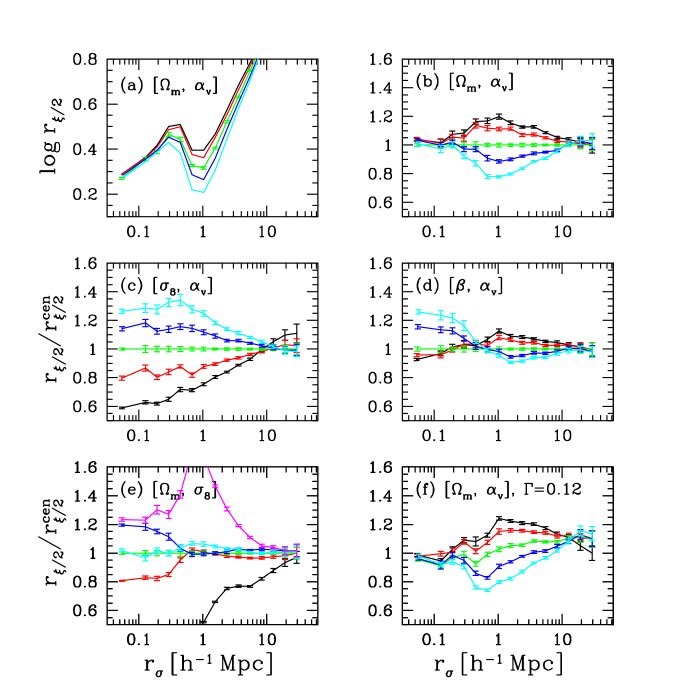
Figure 15: The smalle-scale distortion parameter, $r_{\xi/2}$, as a function of transverse separation. For panels (b) — (f), each curve has been normalized by the values for the central model, while panel (a) plots the curves as $\log\,r_{\xi/2}$ for the constant [$\Omega_{m},\alpha_{v}$] sequence, without normalization. Models run from $\sigma_{8}=0.95$ (black) to $\sigma_{8}=0.6$ (cyan) in panels (a) and (b), from $\Omega_{m}=0.1$ (black) to $\Omega_{m}=0.5$ (cyan) in panel (c), from $\sigma_{8}=0.95$ (black) to $\sigma_{8}=0.6$ (cyan) in panel (d), with the order of the colors being black, red, green, blue, cyan. In panel (e), models are $\alpha_{v}=0$ (black), $\alpha_{v}=0.8$ (red), $\alpha_{v}=1.0$ (green), $\alpha_{v}=1.2$ (blue), $\alpha_{vc}=0.2$ (cyan), and $\alpha_{vc}=1$ (magenta). (f) Models are the same as panel (b), but with $\Gamma=0.12$.

5 Small-Scale Distortion

While the non-linear length scales give some measure of small-scale velocities, we can characterize these velocities more physically and more accurately by focusing on distortions at small $r_{\sigma}$, where they dominate. The traditional measure of small-scale distortions is the pairwise velocity dispersion, but this is not a direct observable; it is extracted from the data by fitting a model that specifies the scale dependence of the mean pairwise velocity of galaxies and the form of the velocity distribution (e.g., Davis & Peebles 1983). We would prefer a quantity that is measured directly from the data, and here we follow the lead of Fisher et  al. (1994), who use $\xi(r_{\pi})$ at fixed, small $r_{\sigma}$. Referring back to Figure 5, we see that $\xi(r_{\pi})$ at small $r_{\sigma}$ is constant for a range of $r_{\pi}$, before turning over at a scale determined by the galaxy velocity dispersion. We can quantify this turnover by the measure $r_{\xi/2}$, the value of $r_{\pi}$ at which the correlation function decreases by a factor of two relative to its value at $r_{\pi}=0$. More generally, one could use the shape of $\xi(r_{\pi})/\xi(r_{\pi}=0)$ over some range of the line-of-sight separation, scaling by $\xi(r_{\pi}=0)$ to remove the sensitivity of the distortion measure to the exact value of the real-space correlation function.

Figure 15a plots $r_{\xi/2}$ against $r_{\sigma}$ for the [$\Omega_{m},\alpha_{v}$] sequence. All the curves have a characteristic wave pattern, which rises to a maximum at $r_{\sigma}\sim 0.6$ $h^{-1}$Mpc and reaches a minimum at $r_{\sigma}\sim 1$ $h^{-1}$Mpc. The rise at small separation is the result of including one-halo galaxy pairs from increasingly more massive halos with higher velocity dispersions. The minimum at 1 $h^{-1}$Mpc occurs near the one-halo to two-halo transition in the real-space $\xi_{R}(r)$. At this separation, two-halo pairs come largely from the central galaxies of lower mass halos, so they do not have an internal dispersion contribution, and the halo pairwise velocities themselves are relatively low. At $r_{\sigma}>1$ $h^{-1}$Mpc, all curves monotonically increase, as the internal dispersions of large halos again start to contribute and the pairwise dispersion of halos themselves increases. To highlight the differences between the models, panels (b) — (f) plot five model sequences where all the curves have been normalized by the values for the central model $(\Omega_{m}=0.3,\sigma_{8}=0.8,\alpha_{v}=1,\alpha_{vc}=0)$. Panels (b) — (e) show the standard suite from Table 2 and earlier figures. In panel (b), with fixed $\Omega_{m}$ and $\alpha_{v}$, changing $\sigma_{8}$ has little effect on $r_{\xi/2}$ at $r_{\sigma}\leq 0.2$ $h^{-1}$Mpc. This separation is small enough that rare, high-mass halos do not contribute a large fraction of the one-halo galaxy pairs relative to the pairs contributed by halos with mass $M_{h}\approx M_{1}$, where $\sigma_{8}$ has little effect on the halo mass function. The value of $\sigma_{8}$ has a large impact on $r_{\xi/2}$ at $r_{\sigma}\sim 1$ $h^{-1}$Mpc, the location of the one-halo to two-halo transition. More high mass halos create more large separation one-halo pairs, extending the one-halo $\xi_{R}(r)$ to larger $r$. These pairs have large velocity dispersion and are therefore spread out along the line of sight, increasing $r_{\xi/2}$.

In panel (c), with fixed $\sigma_{8}$ and $\alpha_{v}$, changing $\Omega_{m}$ affects $r_{\xi/2}$ at all $r_{\sigma}\la 10$ $h^{-1}$Mpc. Higher $\Omega_{m}$ increases both halo pairwise velocities and internal velocity dispersions, thus increasing $r_{\xi/2}$ on all scales where dispersion dominates over coherent flows. Panel (d) shows models with constant $\beta$ and $\alpha_{v}$, and thus constant large-scale anisotropy. As expected from the previous results, higher $\Omega_{m}$ models have larger $r_{\xi/2}$ at $r_{\sigma}\sim 0.1$ $h^{-1}$Mpc, where $\sigma_{8}$ has little impact. At $r_{\sigma}\sim 1$ $h^{-1}$Mpc, the higher $\Omega_{m}$ models (with lower $\sigma_{8}$) have smaller $r_{\xi/2}$; the depression seen in panel (b) wins out over the enhancement in panel (c). Thus, at fixed $\beta$ and $\alpha_{v}$, the small scale distortions can break the degeneracy between $\Omega_{m}$ and $\sigma_{8}$.

Panel (e) shows models with varying $\alpha_{v}$ but constant $\Omega_{m}$ and $\sigma_{8}$ (and thus constant $\beta$). Not surprisingly, the $\alpha_{v}=0$ model has very small values of $r_{\xi/2}$ relative to the central model at scales less than 10 $h^{-1}$Mpc. The effect of moderate velocity bias is most significant at the smallest $r_{\sigma}$, with 20% changes in $r_{\xi/2}$ at $r_{\sigma}=0.1$ $h^{-1}$Mpc for $\alpha_{v}=1.2$ or 0.8. However, these $\alpha_{v}$ variations have little impact at large $r_{\sigma}$, where 20% changes of internal velocity dispersions are small compared to halo velocities themselves, and the effect is essentially zero at $r_{\sigma}\sim 1$ $h^{-1}$Mpc. At this separation, two-halo pairs begin to dominate $\xi(r_{\sigma},r_{\pi})$, but $r_{\sigma}$ is still smaller than the virial radii of large halos. Most pairs therefore come from halos that contain a central galaxy and no satellites, and the value of $\alpha_{v}$ has no effect. Central galaxy velocities have maximum effect at the $\sim 1$ $h^{-1}$Mpc scale, for the same reason. Setting $\alpha_{vc}=0.2$ boosts $r_{\xi/2}$ by 5-10% at this $r_{\sigma}$, while treating central galaxies like satellites ($\alpha_{vc}=1$) boosts it by a factor of two.

Panel (f) plots the results for the constant [$\Omega_{m},\alpha_{v}$] sequence with $\Gamma=0.12$, once again normalized by the $\Gamma=0.2$ central model. As in panel (b), $\sigma_{8}$ has minimal effect at small scales and makes the most difference at $r_{\sigma}\sim 1-2$ $h^{-1}$Mpc. The higher $r_{\xi/2}$ at large $r_{\sigma}$ in the $\Gamma=0.12$ models probably reflects the shallower real-space correlation function at these scales.

Figure 15 demonstrates that $r_{\xi/2}$ is a robust diagnostic for $\Omega_{m}$ and $\alpha_{v}$ when $r_{\sigma}$ is small, independent of $\sigma_{8}$ or $\Gamma$. In figure 16a, the upper points plot $r_{\xi/2}(0.1)$ against $\Omega_{m}\alpha_{v}^{2}$ for all of the $\Gamma=0.2$ models (except those with $\alpha_{v}=0$ and $\alpha_{vc}=1$). The data follow a power law with a slope of 0.46 and minimal scatter. For one-halo pairs, the redshift-space separation depends on relative velocities, which are proportional to $\Omega_{m}^{1/2}\alpha_{v}$, and one might therefore expect a slope of 0.5. Because there is a small two-halo contribution to $\xi(r_{\sigma},r_{\pi})$ at these separations, the slope deviates slightly from this expectation. The data for $\Gamma=0.12$ follow a similar power law, but with a normalization $\sim 7\%$ lower, as expected from the results in Figure 15f. This offset may arise partly from the difference in the real-space correlation function, which is shallower for $\Gamma=0.12$, and partly from the difference in the halo mass function, which changes the relative importance of pairs from different halos.

The values of $\beta$ and $r_{\xi/2}(0.1)$ provide two observable constraints in our three-dimensional $(\Omega_{m},\sigma_{8},\alpha_{v})$ parameter space, measuring the combinations $\sigma_{8}\Omega_{m}^{0.6}$ and $\Omega_{m}\alpha_{v}^{2}$. A measurement of $r_{\xi/2}$ at somewhat larger $r_{\sigma}$ has the possibility of providing a third constraint on a different combination of these parameters. Based on the power-law fit in Figure 16a, each constant-$\beta$ model was given the value of $\alpha_{v}$ required to match $r_{\xi/2}(0.1)$ of the central model. Relative to Figure 15d at fixed [$\beta,\alpha_{v}$], this scaling brings curves together at $r_{\sigma}<1$ $h^{-1}$Mpc, but it makes little difference at larger separations where $\alpha_{v}$ has little effect. Differentiating between adjacent models requires high precision in the measurements, but there is a clear, 20% separation between the low and high values of $\sigma_{8}$ with this diagnostic. In Figure 16b, we plot $r_{\xi/2}$ against $\sigma_{8}$ for $r_{\sigma}=3,4$, and 5 $h^{-1}$Mpc. At each transverse separation, there is a monotonic, nearly linear trend with $\sigma_{8}$ once $\beta$ and $r_{\xi/2}(0.1)$ have been fixed. These results allow for unambiguous determination of $\sigma_{8}$, breaking the third and last degeneracy in the parameter space.

Figure 16b assumes $\alpha_{vc}=0$, and central galaxy velocities could interfere with this approach to breaking degeneracies. For example, adopting $\alpha_{vc}=0.2$ increases $r_{\xi/2}(0.1)$ by $\sim 5\%$, which is of order the effect of changing $\sigma_{8}$ by 0.1. However, the effects of moderate $\alpha_{vc}$ on this measure go away at scales larger than 3 $h^{-1}$Mpc, where there is still clear model differentiation in Figures 15d and 16b. As we have already noted, physical arguments and hydrodynamic simulations support the assumption of low $\alpha_{vc}$, but further theoretical and observational investigation of this point is warranted.

Figure 16: Diagnostic power of the small scale distortion measure. (a) Points show $r_{\xi/2}(0.1)$ against $\Omega_{m}\alpha_{v}^{2}$ for all of the $\Gamma=0.2$ models, except $\alpha_{v}=0$ and $\alpha_{vc}=1$. The upper line shows a least-squares fit, $r_{\xi/2}(0.1)=3.7(\Omega_{m}\alpha_{v}^{2})^{0.46}$, with $\chi^{2}_{d.o.f.}=1.9$. The lower points, shifted down by 0.2 dex for visual clarity, show the $\Gamma=0.12$ results. These data lie $\sim 7\%$ below the (shifted) line. (b) Dependence of $r_{\xi/2}$ on $\sigma_{8}$ for models in which both the large scale distortions ($\beta=0.46$) and the small-scale distortions [$r_{\xi/2}(0.1)=2.0$ $h^{-1}$Mpc] are fixed to the same values. Circles, squares, and triangles represent $r_{\sigma}=3,4$ and 5 $h^{-1}$Mpc, respectively.

6 Discussion

Our results provide a blueprint for obtaining constraints in the $(\Omega_{m},\sigma_{8},\alpha_{v})$ parameter space from measurements of clustering anisotropy in redshift space. For each model in the parameter space, one first chooses HOD parameters to reproduce measurements of the projected galaxy correlation function $w_{p}(r_{p})$, which depends only on the real-space correlation function $\xi_{R}(r)$. If the assumed power spectrum shape is correct, it will generally be possible to match $w_{p}(r_{p})$ well for a wide range of $\sigma_{8}$ and $\Omega_{m}$. At large scales, the anisotropy ratios $P_{0/R}$, $P_{2/0}$, $\xi_{0/R}$ or $Q_{\xi}$ then depend on $\beta\equiv\Omega_{m}^{0.6}/b_{g}$, where $b_{g}^{2}=\xi_{g}/\xi_{m}$ is a monotonically decreasing function of $\sigma_{8}$ for fixed galaxy clustering (see §4.4). These measures scale with cosmological parameters as predicted by linear theory and the linear bias model (Kaiser 1987), even though these approximations do not provide an accurate description of anisotropy on most scales accessible to observations or to our simulations. One can estimate $\beta$ by fitting $P_{0/R}$, $P_{2/0}$, or $Q_{\xi}$ as a function of scale using our equations (16), (17), and (18), or by measuring $\xi_{0/R}$ at $r\geq 10$ $h^{-1}$Mpc and correcting for the $\sim 6\%$ bias of linear theory (see Figure 12). The turnover scales in the fitting functions depend on the velocity bias $\alpha_{v}$, but they can be measured directly from the anisotropy ratios, so the $\beta$ estimates themselves are largely independent of $\alpha_{v}$.

The turnover scales can be used to break degeneracies in the parameter space, but the line-of-sight correlation function $\xi(r_{\pi})$ at fixed, small $r_{\sigma}$ provides a more direct measure of velocity distortions in the highly non-linear regime. In particular, for small $r_{\sigma}$ the scale $r_{\xi/2}$ defined by $\xi(r_{\sigma},r_{\xi/2})=0.5\times\xi(r_{\sigma},0)$, quantifies the typical length of “fingers-of-god,” and hence the characteristic amplitude of pairwise velocity dispersions. At $r_{\sigma}\sim 0.1$ $h^{-1}$Mpc, where most pairs come from intermediate mass halos, we find that $r_{\xi/2}$ depends on $\Omega_{m}\alpha_{v}^{2}$ with essentially no dependence on $\sigma_{8}$. At $r_{\sigma}\sim 1-5$ $h^{-1}$Mpc, $r_{\xi/2}$ has a significant dependence on $\sigma_{8}$ even at fixed $\beta$ and $\alpha_{v}$, with $\Delta\sigma_{8}\sim 0.1$ corresponding to $\Delta r_{\xi/2}\sim 5\%$. Therefore, one can in principle use measurements of large-scale anisotropy and $\xi(r_{\pi})$ at $r_{\sigma}\sim 0.1-5$ $h^{-1}$Mpc to separately determine the values of $\Omega_{m}$, $\sigma_{8}$, and $\alpha_{v}$. Alternatively, one can measure $\beta$ and $\Omega_{m}\alpha_{v}^{2}$ as described above and adopt theoretical priors on $\alpha_{v}$ from hydrodynamic simulations of galaxy formation (e.g., Berlind et  al. 2003), or combine redshift-space distortions with other observables that constrain different combinations of $\sigma_{8}$ and $\Omega_{m}$. For example, galaxy-galaxy lensing measurements constrain $\sigma_{8}\Omega_{m}$ (instead of $\sigma_{8}\Omega_{m}^{0.6}$) from the ratio of the galaxy-mass correlation function to the galaxy autocorrelation function (Sheldon et  al. 2004). The galaxy bispectrum can yield a direct estimate of $\sigma_{8}$ by determining the large-scale galaxy bias factor (Fry 1994; Verde et  al. 2002).

Our blueprint has significant advantages relative to the linear-exponential model or the alternative fitting procedure of HC99. First, our approach is more accurate for a wide range of cosmological models (Figs. 6, 12). Averaging over both values of $\Gamma$ used, our fitting function for $P_{0/R}$ yields $\beta$ with an rms error of 1.6% for the range of models presented. For the $P_{2/0}$ and $Q_{\xi}$ diagnostics, the fitting functions yield rms errors of 4.1% and 3.9% respectively. Second, our approach makes use of the small-scale anisotropy as a tool for breaking parameter degeneracies, instead of treating the galaxy dispersion as a nuisance parameter. Constraints on $\sigma_{8}$ and $\alpha_{v}$ from these small scale measures can be used to further improve the $\beta$ estimate.

The fitting formulas presented here are designed to allow straightforward parameter estimation given measurements of $\xi(r_{\sigma},r_{\pi})$ and $P_{Z}(k,\mu)$. Alternatively, one can use simulations to calibrate a fully analytic description of redshift-space anisotropy, in which case one can fit data directly using $\Omega_{m}$, $\sigma_{8}$, and $\alpha_{v}$ as the fitting parameters. We will develop such a model in Paper II; achieving the accuracy demanded by data sets like the SDSS and the 2dFGRS is not easy, but it is possible. The analytic method is more flexible than the fitting formula approach, allowing one to take more complete advantage of information in $\xi(r_{\sigma},r_{\pi})$ or $P_{Z}(k,\mu)$. At the opposite extreme, one can circumvent analytic formulations entirely and fit data by directly populating halos of N-body simulations and measuring anisotropy, using the $\Omega_{m}$-scaling technique of this paper to improve efficiency. With large volume simulations that resolve the necessary halo masses, this method should achieve the highest accuracy because it fully describes non-linear halo clustering, and it can address corrections to the distant-observer approximation and other technical issues that are difficult to model analytically. In practice, it will probably be best to use the fitting formulas or an analytic model to locate the most interesting regions of parameter space, then use focused numerical simulations to check and refine estimates.

For the $\alpha_{v}=0$ model, large-scale anisotropy measures agree reasonably with linear theory over a substantial range in scale. This result suggests that FOG compression plus linear theory is a viable alternative approach to estimating $\beta$. Assessing the systematic uncertainties of this method requires tests with realistic mock catalogs that quantify the ability of the FOG compression algorithm to correctly identify and compress true FOGs in galaxy survey data.

There are several limitations to our blueprint. With two exceptions, we have assumed that central galaxies move with the center of mass of the halo, i.e. $\alpha_{vc}=0$. Changing $\alpha_{vc}$ to 0.2 makes minimal difference in both the large scale measures and $r_{\xi/2}$. However, setting $\alpha_{vc}\approx 1$ makes a considerable difference. Current hydrodynamical simulations (Berlind et  al. 2003) suggest $\alpha_{vc}\la 0.2$ is a reasonable assumption, but the issue merits further investigation because of its significant impact on redshift-space anisotropy modeling. Analysis of SDSS galaxies shows that central-satellite galaxy pairs indeed have a narrower velocity spread than satellite-satellite pairs (T. McKay et  al., in preparation). We have also assumed that $\alpha_{v}$ is independent of halo mass. This assumption should be adequate because most one-halo pairs come from a limited range of halo masses; low-mass halos have no satellites, and high-mass halos are rare. To significantly alter our results, $\alpha_{v}$ would need to depend strongly on mass in the relatively narrow range $M_{1}/2-5M_{1}$, and even then its effect might be well represented by an average value. The weak mass dependence seen in the simulations analyzed by Berlind et  al. (2003) does not affect the results here, but the question again merits investigation in future hydrodynamic studies of galaxy formation. One can also test for mass dependence of $\alpha_{v}$ by comparing the predicted and observed scalings of group velocity dispersions with group richness.

The experiments illustrated in Figure 7 show that changing the details of the HOD, or the assumption about spatial bias within halos, has negligible impact on redshift-space distortions provided one matches the same real-space clustering. However, our investigation of these points is not exhaustive. Effects of changing $\alpha_{vc}$, making $\alpha_{v}$ mass-dependent, or changing HOD prescriptions while maintaining $\xi_{R}(r)$ can all be examined in more detail using the analytic model of Paper II.

The simulations presented in this work have less dynamic range than is ideal. At the largest scales, our numerical predictions are less precise than the measurement precision achievable with 2dFGRS or SDSS data, though not by a large factor. We have focused on predictions for luminosity-threshold galaxy samples with space density $5.6\times 10^{-3}\,($$h^{-1}$Mpc$)^{-3}$, corresponding roughly to $M_{r}<-20+5\log h$. To make predictions or test fitting formulas for fainter galaxies, which occupy less massive halos, one would need higher resolution simulations but similar simulation volumes. To get precise results for more luminous galaxies that reside in rare, massive halos, one would need larger simulation volumes, though the mass resolution required is lower. The analytic model described in Paper II can easily be applied to samples with different luminosity or color selection and correspondingly different HODs, and it automatically extends to large scales. However, additional simulations will be needed to test the accuracy of the analytic model in these regimes.

The monopole-to-real space ratios, $P_{0/R}$ and $\xi_{0/R}$, have smaller systematic errors as estimators of $\beta$ than the quadrupole-to-monopole ratios $P_{2/0}$ and $Q_{\xi}$. However, we have not addressed the problem of estimating $\xi_{R}(r)$ or $P_{R}(k)$ from data. Techniques for estimating these quantities exist (e.g., Davis & Peebles 1983; Hamilton et  al. 2000; Zehavi et  al. 2004b; Tegmark et  al. 2004a), but we do not yet know whether they are accurate at the $\sim 1-2\%$ level required if they are not to contribute significantly to uncertainties in the estimates of $\beta$.

Despite these limitations, our results demonstrate that HOD modeling can substantially improve the accuracy and precision of redshift-space distortion analysis by replacing ad hoc extensions of linear perturbation theory with a complete, fully non-linear description of dark matter dynamics and galaxy bias. This level of sophistication is required to take full advantage of data provided by the 2dFGRS and SDSS. Precise cosmological constraints from galaxy clustering complement those from other cosmological observables like CMB anisotropy, gravitational lensing, the Lyman-$\alpha$ forest, or Type Ia supernovae. They thus enhance the opportunity to detect departures from the simplest $\Lambda$CDM model, which could provide insight into the physics of dark energy or the origin of primordial fluctuations.

References

- Abazajian et al. (2004) Abazajian, A., et al. ApJ (submitted), astro-ph/0408003
- Bean et al. (1983) Bean, A. J., Ellis, R. S., Shanks, T., Efstathiou, G., & Peterson, B. A. 1983, MNRAS, 205, 605
- Benson (2001) Benson, A. J. 2001, MNRAS, 325, 1039
- Benson et al. (2000) Benson, A. J., Cole, S., Frenk, C. S., Baugh, C. M., & Lacey, C. G. 2000, MRNAS, 311, 793
- Berlind & Weinberg (2002) Berlind, A. A., & Weinberg, D. H. 2002, ApJ, 575, 587
- Berlind et al. (2003) Berlind, A. A., Weinberg, D. H., Benson, A. J., Baugh, C. M., Cole, S., Davé, R., Frenk, C. S., Katz, A., & Lacey, C. G. 2003, ApJ, 593, 1
- Berlind et al. (2001) Berlind, A. A., Narayanan, V. K., & Weinberg, D. H. 2001, ApJ, 549, 688
- Blanton et al. (2003) Blanton, M. R., et al. 2003, ApJ, 592, 819
- Bullock et al. (2001) Bullock, J. S., Kolatt, T. S., Sigad, Y., Somerville, R. S., Klypin, A. A., Primack, J. R., Dekel, A. 2001, MNRAS, 321, 559
- Colless et al. (2001) Colless, M. et. al. 2001, MNRAS, 328, 1039
- Cole et al. (1994) Cole, S., Fisher, K. B., & Weinberg, D. H. 1994, MNRAS, 267, 785
- Cole et al. (1995) Cole, S., Fisher, K. B., & Weinberg, D. H. 1995, MNRAS, 275, 575
- Cooray (2004) Cooray, A., 2004, MNRAS, 348, 250
- Cooray & Sheth (2002) Cooray, A. & Sheth, R. K. 2002, Phys. Rep., 372, 1
- Davis et al. (1978) Davis, M., Geller, M. J., & Huchra, J. 1978, ApJ, 221, 1
- Davis & Peebles (1983) Davis, M. & Peebles, P. J. E. 1983, ApJ, 267, 465
- Davis et al. (1985) Davis, M., Efstathiou, G., Frenk, C. S., & White, S. D. M. 1985, ApJ, 292, 371
- Efstathiou et al. (1992) Efstathiou, G., Bond, J. R., & White, S. D. M. 1992, MNRAS, 258, 1
- Faltenbacher et al. (2004) Faltenbacher, A., Kravtsov, A. V., Nagai, D., & Gottlöber, S. 2004, MNRAS (submitted), astro-ph/0408488
- Fisher et al. (1994) Fisher, K. B., Davis, M., Strauss, M. A., Yahil, A., & Huchra, J. P. 1994, MNRAS, 267, 927
- Fisher & Nusser (1996) Fisher, K. B. & Nusser, A 1996, MNRAS, 279, L1
- Fry (1994) Fry, J. N. 1994, Phys. Rev. Lett., 73, 215
- Hamilton (1992) Hamilton, A. J. S. 1992, ApJ, 385, L5
- Hamilton (1998) Hamilton, A. J. S. 1998, in The Evolving Universe, ed. D. Hamilton (Dordrecht: Kluwer), 185
- Hamilton et al. (2000) Hamilton, A. J. S., Tegmark, M., & Padmanabhan, N. 2000, MNRAS, L317, 23
- Hatton & Cole (1998) Hatton, S. & Cole, S. 1998, MNRAS, 296, 10
- Hatton & Cole (1999) Hatton, S. & Cole, S. 1999, MNRAS, 310, 1137
- Hawkins et al. (2003) Hawkins, E., et al. 2003, MNRAS, 346, 78
- Hu & Kravtsov (2003) Hu, W. & Kravtsov, A. V., 2003, ApJ, 584, 702
- Jing et al. (1998) Jing, Y. P., Mo, H. J., & Börner, G. 1998, ApJ, 494, 1
- Jenkins et al. (2001) Jenkins, A., Frenk, C. S., White, S. D. M., Colberg, J. M., Cole, S., Evrard, A. E., Couchman, H. M. P., & Yoshida, N. 2001, MNRAS, 321, 372
- Kaiser (1987) Kaiser, N. 1987, MNRAS, 227, 1
- Kang et al. (2002) Kang, X., Jing, Y. P., Mo, H. J., & Börner, G. 2002 MNRAS, 336, 892
- Kauffmann et al. (1997) Kauffmann, G., Nusser, A., & Steinmetz, M. 1997, MNRAS, 286, 795
- Kravtsov et al. (2004) Kravtsov, A. V., Berlind, A. A., Wechsler, R. H., Klypin, A. A., Gottlöber, S., Allgood, B., Primack, J. R. 2004, ApJ, 609, 35
- Kuhlen et al. (2004) Kuhlen, M., Strigari, L. E., Zentner, A. R., Bullock, J. S., Primack, J. R., 2004, ApJ (submitted), astro-ph/0405143
- Ma & Fry (2000) Ma, C. & Fry, J. N. 2000, ApJ, 543, 503
- Melott (1983) Melott, A. L. 1983, ApJ, 264, 59
- Mo et al. (2004) Mo, H. J., Yang, X., & van den Bosch, F. C. 2004, MNRAS, 349, 205
- Navarro, Frenk, & White (1997) Navarro, J. F., Frenk, C. S., & White, S. D. M. 1997, ApJ, 490, 493
- Park (1990) Park, C. 1990, MNRAS, 242, 59
- Park et al. (1994) Park, C., Vogeley, M. S., Geller, M. J., & Huchra, J. P. 1994, ApJ, 431, 569
- Peacock & Dodds (1994) Peacock, J. A. & Dodds, S. 1994, MNRAS, 267, 1020
- Peacock et al. (2001) Peacock, J. A., et al. 2001, Nature, 410, 169
- Peacock & Smith (2001) Peacock, J. A., Smith, R. E. 2000, MNRAS, 318, 1144
- Peebles (1976) Peebles, P. J. E. 1976, ApJ, 205, L109
- Peebles (1979) Peebles, P. J. E. 1979, AJ, 84, 730
- Percival et al. (2002) Percival, W. J. et al. 2002, MNRAS, 337, 1068
- Sargent & Turner (1977) Sargent, W. L. W. & Turner, E. L. 1977, ApJ, 212 L3
- Scoccimarro et al. (2001) Scoccimarro, R., Sheth, R. K., Hui, L., & Jain, B. 2001, ApJ, 546, 20
- Scoccimarro (2004) Scoccimarro, R. 2004, Phys. Rev. D (in press), astro-ph/0407214
- Seljak & Zaldarriaga (1996) Seljak U. & Zaldarriaga M. 1996, ApJ, 469, 437
- Seljak (2000) Seljak, U. 2000, MNRAS, 318, 203
- Seljak (2001) Seljak, U. 2001, MNRAS, 325, 1359
- Sheldon et al. (2004) Sheldon, E., et al. 2004, AJ, 127, 2544
- Sheth et al. (2001) Sheth, R. K., Hui, L., Diaferio, A., & Scoccimarro, R. 2001, MNRAS, 325, 1288
- Sheth & Diaferio (2001) Sheth, R. K. & Diaferio, A. 2001, MNRAS, 322, 901
- Spergel et al. (2003) Spergel, D. N., et al. 2003, ApJ, 148, 175
- Springel, Yoshida, & White (2001) Springel, V., Yoshida, N., & White, S. D. M. 2001 NewA, 6, 79
- Strauss & Willick (1995) Strauss, M. A. & Willick, J. A. 1995 Phys. Rep., 261, 271
- Strauss et al. (2002) Strauss, M. A., et al. 2002, AJ, 124, 1810
- Tegmark et al. (2004a) Tegmark, M., et al. 2004a, ApJ, 606, 702
- Tegmark et al. (2004b) Tegmark, M., et al. 2004b, Phys. Rev. D, 69, 103501
- Tinker et al. (2004) Tinker, J. L., Weinberg, D. H., Zheng, Z., & Zehavi, I. 2004, ApJ (submitted), astro-ph/0411777
- van den Bosch et al. (2003) van den Bosch, F. C., Yang, X., & Mo, H. J. 2003, MNRAS, 345, 723
- Verde et al. (2002) Verde, L., et al. 2002, MNRAS, 335, 432
- White (2001) White, M. 2001, MNRAS, 321, 1
- White et al. (2001) White, M., Hernquist, L., & Springel, V. 2001, ApJ, 550, L129
- Yang et al. (2004) Yang, X., Mo, H. J., Jing, Y. P., van den Bosch, F. C., & Chu, X. Q. 2004, MNRAS, 350, 1153
- York et al. (2000) York, D., et al. 2000, AJ, 120, 1579
- Yoshikawa et al. (2001) Yoshikawa, K., Taruya, A., Jing, Y. P., & Suto, Y. 2001, ApJ, 558, 520
- Zehavi et al. (2004a) Zehavi, I., et al. 2004a, ApJ, 608, 16
- Zehavi et al. (2004b) Zehavi, I., et al. 2004b, ApJ (submitted), astro-ph/0408569
- Zheng (2004) Zheng, Z. 2004, ApJ, 610, 61
- Zheng et al. (2004) Zheng, Z., Berlind, A. A., Weinberg, D. H., Benson, A. J., Baugh, C. M., Cole, S., Davé, R., Frenk, C. S., Katz, A., & Lacey, C. G. 2004, ApJ (submitted), astro-ph/0408569
- Zheng et al. (2002) Zheng, Z., Tinker, J. L., Weinberg, D. H., & Berlind, A. A. 2002, ApJ, 575, 617