Exactly Solvable SFT Inspired Phantom Model

Abstract

An exact solution to the Friedmann equations with a string inspired phantom scalar matter field is constructed and the absence of the “Big Rip” singularity is shown explicitly. The notable features of the concerned model are a ghost sign of the kinetic term and a special polynomial form of the effective tachyon potential. The constructed solution is stable with respect to small fluctuations of the initial conditions and special deviations of the form of the potential.

1 INTRODUCTION

The combined analysis of the type Ia supernovae, galaxy clusters measurements and WMAP (Wilkinson Microwave Anisotropy Probe) data brings out clearly an evidence of the accelerated expansion of the Universe [1]-[4]. The cosmological acceleration strongly indicates that the present day Universe is dominated by a smoothly distributed slowly varying cosmic fluid with a negative pressure, the so-called dark energy [5]-[8] (alternative approaches are presented, for example, in [9]).

To specify different types of cosmic fluids one usually uses a phenomenological relation between the pressure density $p$ and the energy density $\varrho$, corresponding to each component of fluid

$$p=w\varrho,$$

where $w$ is the equation-of-state parameter or, for short, the state parameter. A component with negative $w$ corresponds to the dark energy. Contemporary experiments, including WMAP, give strong support that at present time the dark energy state parameter is close to $-1$ [4], [10]-[14]. In particular, it follows from the current observational bounds [2] that $w$ belongs to the interval:

$$-1.46<w<-0.78.$$

at the $95\%$ confidence level.

From the theoretical point of view the above-mentioned domain of $w$ covers three essentially different cases: $w>-1,~{}w=-1$ and $w<-1$.

• The first case, $w>-1$, is achieved in quintessence models [15]-[22], which are cosmological models with a scalar field. Such types of models are quite acceptable, but there is a question of an origin of the scalar field. To comply with astronomical experimental data this scalar field should be extra light and hence it does not belong to the Standard Model set of fields [23].

• The second case, $w=-1$, is realized by means of the cosmological constant. This scenario is admissible from a general point of view except for a problem of an order of the magnitude of the cosmological constant. It should be $10^{120}$ times less than the natural theoretical prediction [8].

• The third case, $w<-1$, is called a ”phantom” one and can be realized due to a scalar field with a ghost (phantom) kinetic term. In this case all natural energy conditions are violated and there are problems of instability at classical and quantum levels [24]-[44]. Since experimental data do not contradict with a possibility of $w<-1$ and moreover a direct search strategy to test the inequality $w<-1$ has been proposed [45], it is interesting to find a noncontradictory model with the condition $w<-1$ satisfied.

Note the $\kappa$-essence models [19] can have both $w<-1$ and $w\geqslant-1$. At the same time a dynamical transition from the region $w\geqslant-1$ to the region $w<-1$ or vice versa is forbidden under general assumptions [47] and is possible only under special conditions [48].

Let us recall that in models with a constant state parameter $w$, less than $-1$, and the spatially flat Friedmann metric the scale factor tends to infinity and therefore the Universe breaks down at a finite moment of time. This problem is known as the “Big Rip” [26], see also [27]. The simplest way to overcome this difficulty in models with $w<-1$ is to consider a scalar field $\phi$ with a negative time component in the kinetic term [13, 28]. The appearance of a such summand is possible due to quantum effects [49, 31]. However, all proposed models insist of the instability problem.

A possible way to evade the instability problem for models with $w<-1$ is to yield a phantom model as an effective one, arising from a more fundamental theory without a negative kinetic term. In particular, if we consider a model with higher derivatives such as $\phi e^{-\Box}\phi$, then in the simplest approximation: $\phi e^{-\Box}\phi\simeq\phi^{2}-\phi\Box\phi$, such a model gives a kinetic term with a wrong (ghost) sign. It turns out, that such a possibility does appear in the string field theory framework [44]. Since the concerned model is a string theory approximation, all stability problems related to a model with higher derivatives are discarded.

Our goal in the present paper is to construct an analytic solution in a polynomial model, which is close in some approximation to a model arising in the string theory, namely in the theory of a fermionic NSR string with GSO$-$ sector. The scalar field $\phi$ is an open string theory tachyon, which, according to the Sen’s conjecture [21], describes brane decay, at which a slow transition to the stable vacuum, correlating with states of the closed string, takes place. Other dark energy models, which use the brane-world scenarios, are presented in [50].

The notable feature of the model is a ghost sign of the kinetic term and a special form of the potential:

$$V(\phi)=\frac{1}{2}\left(1-\phi^{2}\right)^{2}+\frac{1}{12m_{p}^{2}}\phi^{2}\left(3-\phi^{2}\right)^{2}.$$ (1)

In the first approximation only the first summand in the right hand side of (1) can be obtained from the open string field theory in a flat metric [51] (which corresponds to $m_{p}=\infty$). The second summand allows us to save the form of the interpolating solution obtained in the flat metric for the case of the Friedmann Universe, i.e. at an arbitrary $m_{p}$. Note, that the appearance of higher powers of $\phi$ is possible if we take into account the heavier perturbations of the string [52], but we can not expect to obtain the explicit values of the coefficients of the potential (1) from the string theory. The performed in this paper stability analysis of solutions points out that the constructed solution is an attractive one and there are no essential changes in the behavior of the solutions for some variations of the potential parameters. This gives reasons to assume, that the qualitative behavior of the physical parameters $H,w,q$ in the model with the potential (1) under certain conditions becomes close to the behavior of the corresponding ones in the model with a string theory potential.

The constructed solution has no singular points and becomes the de-Sitter solution at large time. It does not contradict to the general theorems of the relativity theory because the energy conditions are violated in the considered model (this question is discussed in [53]).

The paper is organized as follows. In Section 2 we describe the cosmological model, which is an approximation for the string inspired model, and write down the solutions to the Friedmann equations with the special polynomial potential. In Section 3 we consider the phantom dynamics in detail and find out that our solution describes an accelerating Universe. In Section 4 we study the stability of the solution with respect to variations of initial data and peculiar variations of a form of the potential. In Section 5 we do sum up the obtained results and point out the ways for generalization of the considered model.

2 MODEL

2.1 Equations of motion

Let us consider the gravitational model with a phantom scalar field and the spatially flat Friedmann metric. Since the origin of the phantom field, considering in this paper, is connected with the string field theory we include the typical string mass $M_{s}$ and a dimensionless open string coupling constant $g_{o}$ in the action. The action is:

$$S=\int d^{4}x\sqrt{-g}\left(\frac{M_{p}^{2}}{2M_{s}^{2}}R+\frac{1}{g_{o}^{2}}\left(+\frac{1}{2}g^{\mu\nu}\partial_{\mu}\phi\partial_{\nu}\phi-V(\phi)\right)\right),$$ (2)

where $M_{p}$ is the Planck mass, $g$ is a spatially flat Friedmann metric:

$$ds^{2}={}-dt^{2}+a^{2}(t)\left(dx_{1}^{2}+dx_{2}^{2}+dx_{3}^{2}\right),$$

where $a(t)$ is the scale factor. The coordinates $(t,x_{i})$ and the field $\phi$ are dimensionless. Hereafter we use the dimensionless parameter $m_{p}^{2}={g_{o}^{2}M_{p}^{2}}/{M_{s}^{2}}$.

Independent equations of motion are as follows

$$3H^{2}=\frac{1}{m_{p}^{2}}\>\varrho,\qquad 3H^{2}+2\dot{H}={}-\frac{1}{m_{p}^{2}}\>p.$$ (3)

Here $H$ is the Hubble parameter: $H\equiv\dot{a}(t)/a(t)$ and the dot denotes the time derivative. If the scalar field depends only on time, i.e. $\phi=\phi(t)$, then

$$\varrho={}-\frac{1}{2}\dot{\phi}^{2}+V(\phi),\qquad p={}-\frac{1}{2}\dot{\phi}^{2}-V(\phi).$$ (4)

We recast system (3) to the following form

$$\dot{H}=\frac{1}{2m_{p}^{2}}\dot{\phi}^{2},\qquad 3H^{2}=\frac{1}{m_{p}^{2}}\left(V(\phi)-\frac{1}{2}\dot{\phi}^{2}\right).$$ (5)

Besides of equations (5) one can obtain from the action (2) an equation of motion for the field $\phi$

$$\ddot{\phi}+3H\dot{\phi}-V_{\phi}^{\prime}=0,$$ (6)

where $V_{\phi}^{\prime}\equiv\frac{dV}{d\phi}$. This equation is in fact a consequence of system (3). Expressing $H$ through $\phi$ and $\dot{\phi}$, we obtain

$$\ddot{\phi}+\mathop{\mathrm{sign}}(H)\frac{\sqrt{3}}{m_{p}}\dot{\phi}\sqrt{-\frac{1}{2}\dot{\phi}^{2}+V(\phi)}-V_{\phi}^{\prime}=0.$$ (7)

Here $\mathop{\mathrm{sign}}(H)$ factor selects the proper branch of the square root. The expanding Universe corresponds to $H>0$.

2.2 Connection with the String Theory

At present time one of the possible scenarios of the Universe evolution considers the Universe to be a D3-brane (3 spatial and one time variable) embedded in higher-dimensional space-time. D-branes do naturally emerge in the open string theory (in our case we consider fermionic open strings containing both GSO$+$ and GSO$-$ sectors). The D-brane in question is unstable and does evolve to the stable state. This process is described by the open string dynamics, which ends are attached to the brane (see reviews [52] and references therein). If only the lowest excitation — the tachyon — is taken into account then the D-brane dynamics are described by an action of the open string tachyon. There are two common ways to describe the tachyon behavior: Dirac-Born-Infeld (DBI) approximation and the level truncation scheme in the covariant string field theory [54, 55, 56]. The level truncation method advocated itself checking the Sen’s conjecture and, therefore, it is natural to use it to analyze the dynamics of the D-brane, see [57, 58, 59]. The action for the tachyon resulting from the fermionic string field theory in the approximation of the slow-varying auxiliary field [58] has the form

$$S_{\text{flat}}=\frac{1}{g_{o}^{2}}\int dx\left(-\frac{1}{2}\partial_{\mu}\varphi\partial^{\mu}\varphi+\frac{1}{4}\varphi^{2}-\frac{81}{256}\tilde{\varphi}^{4}\right).$$

where $\varphi$ is the dimensionless tachyon field and the coordinates and the constant $g_{o}$ are also dimensionless. The tilde means an action of the non-local operator $\exp\left(-\log\left(\frac{4}{3\sqrt{3}}\right)\partial^{2}\right)$ on the field $\varphi$. The subscript “flat” hereafter indicates the flat background metric is used. Note that in the bosonic string case the interaction is cubic. For the space homogenous configurations only the dependence on time $\tau$ is left and the action takes the form

$$S_{\text{flat}}^{(\tau)}=\frac{1}{g_{o}^{2}}\int d\tau\left(+\frac{1}{2}\left(\frac{d\varphi}{d\tau}\right)^{2}+\frac{1}{4}\varphi^{2}-\frac{81}{256}\left(e^{\log\left(\frac{4}{3\sqrt{3}}\right)\frac{d^{2}}{d\tau^{2}}}\varphi\right)^{4}\right).$$

Introducing the notation $\phi=\frac{9}{4\sqrt{2}}\exp\left(\log\left(\frac{4}{3\sqrt{3}}\right)\frac{d^{2}}{d\tau^{2}}\right)\varphi$ and $t=\tau/2$, we rewrite the equations of motion obtained from the last action in the following form

$$\left(-\frac{d^{2}}{dt^{2}}+2\right)e^{\tilde{a}\frac{d^{2}}{dt^{2}}}\phi=2\phi^{3},$$

where $\tilde{a}=-\frac{1}{4}\log\left(\frac{4}{3\sqrt{3}}\right)>0$. In fact this equation is integral one since the exponent containing an infinite number of derivatives can be replaced with an integral operator [57] in some class of fields as follows

$$\left(-\frac{d^{2}}{dt^{2}}+2\right)\frac{1}{\sqrt{4\pi\tilde{a}}}\int e^{\frac{\left(t-t^{\prime}\right)^{2}}{4\tilde{a}}}f(t^{\prime})dt^{\prime}=2\phi(t)^{3}.$$ (8)

Note, that equation (8) without the first summand is an equation for the $p$-adic string (in our case $p=3$) [60]. In the latter case the existence of a solution interpolating between vacua has been proved [61]. Previously this solution has been numerically constructed in [62].

Equation (8) was investigated in [58, 59] and an existence of a rolling solution, i.e. a solution interpolating between the two vacua of the potential

$$V_{\text{flat}}(\phi)=\frac{1}{2}\left(1-\phi^{2}\right)^{2}$$ (9)

was shown numerically. It is remarkable that the late time behavior of the rolling solution can be effectively described by a lagrangian with a ghost sign of the kinetic term and the same potential. The corresponding action has the form

$$S_{\text{eff,flat}}^{(t)}=\int dt\left(-\frac{1}{2}\dot{\phi}^{2}-\frac{1}{2}\left(1-\phi^{2}\right)^{2}\right).$$ (10)

As known, the equation of motion derived from the action (10):

$$\ddot{\phi}+2\phi\left(1-\phi^{2}\right)=0$$ (11)

has an interpolating solution — a kink

$$\phi(t)=\tanh(t).$$ (12)

2.3 Construction of solution

System of equations (5) with some polynomial potential $V(\phi)$ is not integrable. The numeric analysis of the Friedmann equations with the potential (9) has been performed in the paper [44]. It is known ( see, for example [33, 63]) that it is always possible to find the potential $V(\phi)$, if either $\phi(t)$ or $H(t)$ are given explicitly.

It is worth to note that our model has common features with models considered in brane-world scenarios (see Appendix). Following [63], we assume, that $H(t)$ is a function of $\phi(t)$, called superpotential, that is $H(t)=W(\phi(t))$. Using equality $\dot{H}=W_{\phi}^{\prime}\dot{\phi}$, we obtain from system (5):

$$\dot{\phi}=2m_{p}^{2}W_{\phi}^{\prime},$$ (13)

$$V=2m_{p}^{4}{W_{\phi}^{\prime}}^{2}+3m_{p}^{2}W^{2}.$$ (14)

Let us find a potential, which corresponds to the field $\phi$ of type (12). This function satisfies the following equation

$$\dot{\phi}=1-\phi^{2},$$ (15)

hence, from (13) it follows

$$W=\frac{1}{2m_{p}^{2}}\left(\phi-\frac{1}{3}{\phi}^{3}\right)+C,$$

where $C$ is an integration constant. Once $W(\phi)$ is known we obtain the potential $V(\phi)$ from (14). Different values of $C$ correspond to different $V(\phi)$. The requirement that $V(\phi)$ is an even function is equivalent to the condition $C=0$. In this case

$$V(\phi)=\frac{1}{2}\left(1-\phi^{2}\right)^{2}+\frac{1}{12m_{p}^{2}}\phi^{2}\left(3-\phi^{2}\right)^{2}.$$ (16)

It can be straightforwardly verified that if $\phi(t)$ is a solution to (13), (14) with some potential $V(\phi)$, then $\phi(-t)$ is a solution as well. For example, $\phi_{2}(t)=\tanh(-t)=-\tanh(t)$ also is a solution to (13), (14) with the potential (16). Indeed these two solutions correspond to the one and the same function $H(t)$, but to the two different functions $W(\phi)$.

We have constructed the potential $V$, using an explicit form of a solution. Now we consider more general problem and look for solutions, starting with the the following two requirements: $\phi(t)$ is a smooth function with nonzero asymptotics $\phi(\pm\infty)=\pm B$ and the superpotential $W(\phi)$ is a polynomial in $\phi$ not more than the third degree. In the first condition we can put $B=1$ without loss of generality. The second condition guarantees that the potential $V(\phi)$ will be a polynomial in $\phi$ and its degree is not more than six. The above conditions allow us to rewrite equation (13) in the following form:

$$\dot{\phi}=\alpha+\beta\phi+\gamma\phi^{2}.$$ (17)

From the asymptotic conditions it follows

$$\gamma=-\alpha,\qquad\beta=0.$$ (18)

Taking into account (18) we solve equation (17) and obtain

$$\phi(t)=\tanh(\alpha(t-t_{0})).$$ (19)

We do not consider another solution: $\phi(t)=\coth(\alpha(t-t_{0}))$, because it is not a smooth function. Thus, up to a scaling and a time shift we obtain a solution, which coincides with the solution in the flat metric. It is evident that the potential obtained from (14) coincides with (16) up to an overall factor. It is interesting that under above-mentioned conditions on a solution and a superpotential, the sixth degree potential is a minimal possibility for existence of an interpolating solution. One can also see, that any solution to the equations of motion in flat space with the fourth degree potential is a solution to the Friedmann equations either with the sixth degree polynomial potential or with a nonpolynomial potential [64].

It is interesting to note that we have built an exact solution without any approximation. One of the standard approaches to the analysis of cosmological solutions in the presence of a scalar field is the so called slow-roll approximation which technically means a neglecting of the terms $\ddot{\phi}$ in equation (6) and $\dot{\phi}^{2}$ in the expression for the energy (4). However, from (15) it follows that for our solution the following relations take place:

$$\ddot{\phi}=-2\phi\left(1-\phi^{2}\right),\qquad\dot{\phi}^{2}=\left(1-\phi^{2}\right)^{2}.$$

It is evident that the slow-roll approximation in this case is valid only when $\phi$ is close to $1$. The above-mentioned approximation describes our solution at very large times and can not be used for its description in the beginning (close to zero) moments of time.

The Hubble parameter for the constructed solution is given by

$$H=\frac{1}{2m_{p}^{2}}\phi\left(1-\frac{1}{3}{\phi}^{2}\right)=\frac{1}{2m_{p}^{2}}\tanh(t)\left(1-\frac{1}{3}\tanh(t)^{2}\right).$$

This parameter goes asymptotically to $1/(3m_{p}^{2})$ when $t\rightarrow\infty$, or equivalently $\phi\rightarrow 1$. Once $H(t)$ is known one readily obtains the scale factor

$$a=a_{0}\frac{e^{\phi^{2}/(12m_{p}^{2})}}{(1-\phi^{2})^{1/(6m_{p}^{2})}}=a_{0}(\cosh(t))^{\frac{1}{3m_{p}^{2}}}\exp\left({\frac{\cosh(t)^{2}-1}{12m_{p}^{2}\cosh(t)^{2}}}\right),$$ (20)

where $a_{0}$ is an arbitrary constant.

3 COSMOLOGICAL CONSEQUENCES

3.1 Acceleration

The function $a(t)$ has the following asymptotic behavior at large $t$:

$$\lim_{t\to\infty}a(t)\sim e^{\frac{1}{3m_{p}^{2}}t}.$$ (21)

It follows from formulae (20) and (21) that the Universe expands with an acceleration. The deceleration parameter is negative and equal to

$$q(t)=-\>\frac{\ddot{a}a}{\dot{a}^{2}}=-\>\frac{2}{\sinh(t)^{2}}-\frac{5+\cosh(4t)}{2(2+\cosh(2t))^{2}}.$$

The corresponding plots are drawn in Fig. 1 (Hereafter we assume $m_{p}=1$ for all plots if something else is not specified explicitly).

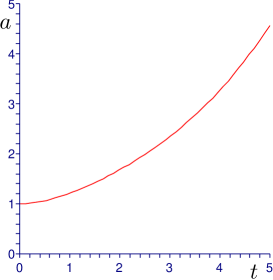
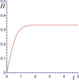
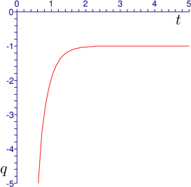
Figure 1: The scale factor $a(t)$ (left), $a_{0}=1$, the Hubble parameter $H(t)$ (center) and the deceleration parameter $q$ (right)

The “jerk” parameter $j=\dot{\ddot{a}}a^{2}/\dot{a}^{3}$ and the “kerk” parameter $k=-\ddot{\ddot{a}}a^{3}/\dot{a}^{4}$ are presented in Fig. 2.

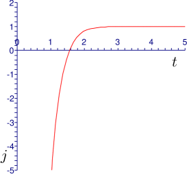
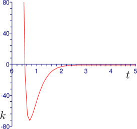
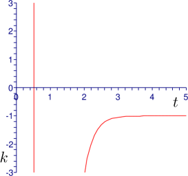
Figure 2: “jerk” parameter (left), “kerk” parameter (center) and its fine structure (right).

Substituting the obtained solution (12) and the potential (16) into expressions for the pressure and energy densities, we obtain

$$p(\phi)=-\left(1-\phi^{2}\right)^{2}-\frac{1}{12m_{p}^{2}}\phi^{2}\left(3-\phi^{2}\right)^{2},\qquad\varrho(\phi)=\frac{1}{12m_{p}^{2}}\phi^{2}\left(3-\phi^{2}\right)^{2}.$$

Therefore, the parameter of state $w$ is given by

$$w\equiv\frac{p}{\varrho}=-1-12m_{p}^{2}\frac{\left(1-\phi^{2}\right)^{2}}{\phi^{2}\left(3-\phi^{2}\right)^{2}}=-1-12m_{p}^{2}\frac{\cosh(t)^{2}}{\sinh(t)^{2}\left(1+2\cosh(t)^{2}\right)^{2}}.$$

Note that the function $w(\phi)$ is less than $-1$ for $|\phi|\neq 1$ and is equal to $-1$ for $|\phi|=1$. Point $\phi=1$ corresponds to infinite future. The plots for the pressure density $p(t)$, the energy density $\varrho(t)$ and the parameter of state $w$ are presented in Fig. 3.

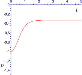
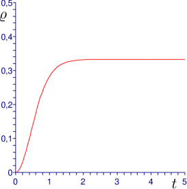
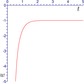
Figure 3: $p(t)$ (left), $\varrho(t)$ (center) and $w(t)$ (right)

Thus, in the considered model of the accelerated expanding Universe the phantom field describes the dark energy with the state parameter $w<-1$.

3.2 Evolution of the exact solution to equation (7)

Solution (12) to equation (7) is a function describing an interpolation of the field $\phi$ from point $-1$ to point $1$ (and not viceversa) with zero initial and final velocities in the potential (16) with a friction proportional to $\mathop{\mathrm{sign}}(H)\sqrt{-\frac{1}{2}\dot{\phi}^{2}+V(\phi)}$, which depends on coordinate and velocity. Factor $\mathop{\mathrm{sign}}(H)$ makes the friction negative for negative $\phi$, i.e. the particle is accelerated by it. Indeed, the expression for friction coefficient is equal to $\phi\left(3-\phi^{2}\right)/(2\sqrt{3}m_{p})$ on the solution for both positive and negative $\phi$.

Let us discuss on the evolution of the exactly constructed solution. A phantom field evolution is equivalent to an evolution of the ordinary field in the flipped potential. The shape of potential $V$ essentially depends on value of $m_{p}$, see Fig. 4, where the flipped potential $-V$ is plotted for different values of $m_{p}$.

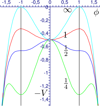
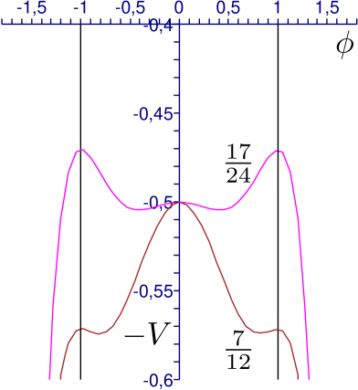
Figure 4: Potential $-V$ for different values of $m_{p}$. The following $m_{p}$ correspond to the curves (top-down direction): $m_{p}^{2}=\infty$, $m_{p}^{2}=1$, $m_{p}^{2}=1/2$ and $m_{p}^{2}=1/4$ in the left plot and $m_{p}^{2}=17/24$ and $m_{p}^{2}=7/12$ in the right plot. Two vertical lines $\phi=\pm 1$ are used as a grid.

To analyze the extrema, let us note the following expressions

$$\begin{split}V(0)&=\frac{1}{2},\qquad V(\pm 1)=\frac{1}{3m_{p}^{2}},\qquad V^{\prime}_{\phi}=\frac{1}{2m_{p}^{2}}\phi\left(1-\phi^{2}\right)\left((3-4m_{p}^{2})-\phi^{2}\right),\\ V^{\prime\prime}_{\phi}(0)&=\frac{3-4m_{p}^{2}}{2m_{p}^{2}},\qquad V^{\prime\prime}_{\phi}(\pm 1)=\frac{2\left(2m_{p}^{2}-1\right)}{m_{p}^{2}}.\end{split}$$ (22)

It is evident from (22) that extrema $\phi=\pm 1$ and $\phi=0$ are independent of $m_{p}$, whereas other extrema are functions of $m_{p}$. Moreover, a particular value of $m_{p}$ determines whether a specific extremum is a maximum or a minimum. Possible values of $m_{p}$ can be separated in the following domains which determine a structure of the flipped potential $-V$ extrema.

• For $m_{p}=\infty$ $V(\phi)$ is a well known double well potential.

• For $\frac{3}{4}\leqslant m_{p}^{2}<\infty$ the flipped potential $-V$, being a 6th degree potential is similar graphically to a flipped double well potential: it has a local minimum in the point $\phi=0$ and maxima in the points $\phi=\pm 1$.

• For $\frac{1}{2}<m_{p}^{2}<\frac{3}{4}$ point $\phi=0$ in the flipped potential becomes a local maximum two more minima appear in the interval $(-1,1)$, developing two wells and one hill on the way of our field $\phi$ during an interpolation from point $-1$ to point $1$, see the right plot in Fig. 4. In more details:

  • For $\frac{2}{3}\leqslant m_{p}^{2}<\frac{3}{4}$ points $\phi=\pm 1$ are not below the point $\phi=0$ in the flipped potential.

  • For $\frac{1}{2}<m_{p}^{2}<\frac{2}{3}$ points $\phi=\pm 1$ are below the point $\phi=0$ in the flipped potential. This means that our field $\phi$ starts at the point $\phi=-1$ with zero initial velocity, rolls down to the well and then climbs up to the hill which is above its initial location. This is counterintuitive while the factor $\mathop{\mathrm{sign}}(H)$ in the friction coefficient is not taken into account. The latter means the friction is negative for negative $\phi$. It seems one can disprove the last statement since it is natural to inverse the time and consider the backward motion. It is easy to resolve this contradiction because in the case of an inverse time function $H$ would have an opposite sign.

• For $m_{p}^{2}=\frac{1}{2}$ the flipped potential has the only extremum which is maximum in the origin and points $\phi=\pm 1$ are inflection points.

• For $m_{p}^{2}<\frac{1}{2}$ two minima, coming from the last multiplier of the expression $V^{\prime}$ (22), go beyond the interval $-1<\phi<1$ and become maxima. Points $\phi=\pm 1$ become minima of the flipped potential. Point $\phi=0$ remains the maximum. In this case field $\phi$ starting at point $\phi=-1$ climbs up to the hill from the very beginning and then rolls down and stops at the point $\phi=1$. Such a behavior seems incredible and becomes real due to a negative friction for negative $\phi$.

Investigating the cosmological evolution of the phantom field we use only the a part of solution (12) starting at the time $t=t_{in}>0$. At this time the field is at the point $\phi_{in}=\phi(t_{in})=\tanh(t_{in})$ and one has to supply an initial velocity $\dot{\phi}(t_{in})=1-\phi_{in}^{2}=1/\cosh^{2}(t_{in})$. For large $m_{p}^{2}$ (weak coupling to the gravity) the phantom field uses an initial kinetic energy to climb up to the hill at $\phi=1$. Increasing a coupling to gravity, i.e. decreasing $m_{p}^{2}$ we lower the height of the hill at the point $\phi=1$ of the flipped potential. For $m_{p}^{2}=2/3$ heights of the hills at points $\phi=0$ and $\phi=1$ become equal and all initial kinetic energy is spent for the work against the friction. For $m_{p}^{2}<2/3$ the friction becomes stronger and the particle has the kinetic energy which is exactly enough to reach the point $\phi=1$ which is now lower than the hill at point $\phi=0$.

4 STABILITY OF SOLUTIONS

4.1 Variation of initial data

Let us consider the behavior of the solution to system (5) in the neighborhood of our exact solution

$$\phi_{0}(t)=\tanh(t),\qquad H_{0}(t)=\frac{1}{2m_{p}^{2}}\tanh(t)\left(1-\frac{1}{3}\tanh(t)^{2}\right),$$

with the aim to analyze its stability. Substituting $\phi(t)=\phi_{0}(t)+\varepsilon\phi_{1}(t)$ and $H(t)=H_{0}(t)+\varepsilon H_{1}(t)$ in system (5), we obtain in the first order of $\varepsilon$ the following equations:

$$\begin{array}[]{@{}rcl@{}}\displaystyle\dot{H}_{1}&\displaystyle=&\displaystyle\frac{1}{m_{p}^{2}}\Bigl{(}1-\tanh(t)^{2}\Bigr{)}\dot{\phi}_{1},\\[10.5275pt] \displaystyle\dot{\phi}_{1}&\displaystyle=&\displaystyle\frac{\left(18-24m_{p}^{2}+24(m_{p}^{2}-1)\tanh(t)^{2}+6\tanh(t)^{4}\right)\tanh(t)}{12m_{p}^{2}\left(1-\tanh(t)^{2}\right)}\phi_{1}-{}\\[7.68222pt] &\displaystyle-&\displaystyle\frac{\left(3-\tanh(t)^{2}\right)\tanh(t)}{1-\tanh(t)^{2}}H_{1}.\\ \end{array}$$ (23)

System (23) has the following solution:

$$\begin{split}\phi_{1}(t)&\displaystyle=2m_{p}^{2}C_{1}\left(1-\tanh(t)^{2}\right)+{}\\ &{}+2m_{p}^{2}C_{2}\frac{2J(t)+(\cosh(2t)-1)(\cosh(t))^{2-\frac{1}{m_{p}^{2}}}e^{\left(\frac{1}{2m_{p}^{2}(\cosh(2t)+1)}\right)}}{\cosh(2t)+1},\\ H_{1}(t)&=C_{1}\left(1-\tanh(t)^{2}\right)^{2}-\frac{4m_{p}^{2}{C}_{2}J(t)}{(\cosh(2t)+1)^{2}},\\ \end{split}$$ (24)

where

$$J(t)=\int_{0}^{t}\!\sinh\left(\tau\right)\left(\cosh(\tau)\right)^{1-1/m_{p}^{2}}\left(2\left(2m_{p}^{2}-1\right)\cosh(\tau)^{2}-1\right)e^{\frac{1}{4m_{p}^{2}\cosh(\tau)^{2}}}d\tau.$$

If $C_{2}=0$, then $H_{1}(t)$ and $\phi_{1}(t)$ are bounded for all $t\in(-\infty,\infty)$ and for all values of $m_{p}$. In this case the solution can be presented in the following form:

$$\phi(t)=\phi_{0}((1+\varepsilon C_{1})t)+{\cal O}(\varepsilon^{2}),\quad H(t)=H_{0}((1+\varepsilon C_{1})t)+{\cal O}(\varepsilon^{2}).$$

Let us consider the case $C_{2}\neq 0$. It is easy to see that if $m_{p}^{2}>1/2$ then $\phi_{1}(t)$ goes to infinity as $t\rightarrow\infty$ and, therefore, our solution is not stable. At $m_{p}^{2}=1/2$ we obtain from (24) that

$$\begin{split}H_{1}(t)&=\left(\tanh(t)^{2}-1\right)^{2}\left(C_{1}-C_{2}J_{2}\right),\\ \phi_{1}(t)&=-\left(\tanh(t)^{2}-1\right)\left(C_{1}-C_{2}J_{2}\right)-\frac{1}{2}C_{2}e^{-\tanh(t)^{2}/2},\end{split}$$

where $J_{2}=\int_{0}^{t}\!{e^{-\tanh(\tau)^{2}/2}}\tanh(\tau){d\tau}$. Thus, $H_{1}$ and $\phi_{1}$ are bounded functions. For $m_{p}^{2}<1/2$, $\phi_{1}(t)$ and $H_{1}(t)$ are bounded functions as well. Thus we obtain that our solutions are stable, the first corrections are bounded, if $m_{p}^{2}\leqslant 1/2$. We remind, that for $m_{p}^{2}<1/2$ points $\phi=\pm 1$ are minima, and for $m_{p}^{2}=1/2$ these points are inflection ones.

To study a behavior of solutions with initial conditions much distinct from the initial conditions of the exact solutions and to answer the question whether the obtained trajectory is an attractive or repulsive one, we construct phase portraits for various values of $m_{p}^{2}$.

Note, that $H(t)$ is a real function. It gives a restriction on the maximal value of $\dot{\phi}(t)^{2}$, namely, for all $\phi$ the inequality that $\dot{\phi}^{2}\leqslant 2V(\phi)$ is hold. For example, let $\phi(0)=0$ then only solutions with $\dot{\phi}(0)\leqslant 1$ have the physical sense. In other words our exact solution starts from this point with the maximal possible speed.

We can not find exact solutions to system (5) with initial conditions $\phi(0)=0$ and $|\dot{\phi}(0)|<1$, and thus we present the results of numeric calculations.

In Fig. 5 phase portraits for $m_{p}>1/2$ are presented, i.e. in the domain of instability of our solution. One can see on the graphs that evolution of solutions comes to the end at points of a minimum of flip potential $-V$, namely at zero for $m_{p}^{2}=100$ and $m_{p}^{2}=1$ and at the point $\phi=\sqrt{2/3}\approx 0.816$ for $m_{p}^{2}=7/12$ (see. Fig. 4).

$\qquad\qquad m_{p}^{2}=100$, $m_{p}^{2}=1$, $m_{p}^{2}=7/12\qquad\qquad$

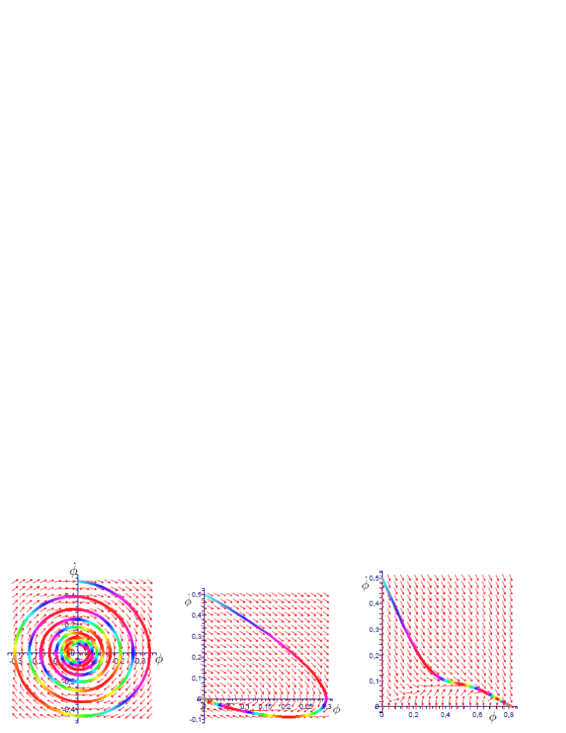
Figure 5: Phase portraits for different values of $m_{p}^{2}>1/2$. Thick lines strokes depict solutions with the initial condition $\dot{\phi}(0)=1/2$.

Let’s consider phase portraits at $m_{p}^{2}\leqslant 1/2$, presented in Fig. 6. In the case $m_{p}^{2}=1/2$ when $\phi=\pm 1$ are inflection points, a solution with the initial speed $\dot{\phi}(0)=1/2$, as well as the exact solution tends to the point $\phi=1$, however coincides with it only in this point. For $m_{p}^{2}=1/4$ and $m_{p}^{2}=1/100$ we see, that the numeric solution is close to the exact solution for $\phi<1$, and the less $m_{p}^{2}$ the less is the value of $\phi$, at which solutions with initial speeds $\dot{\phi}(0)=1/2$ and $\dot{\phi}(0)=1$ get an identical speed.

$\qquad\qquad m_{p}^{2}=1/2$, $m_{p}^{2}=1/4$, $m_{p}^{2}=1/100\qquad\qquad$

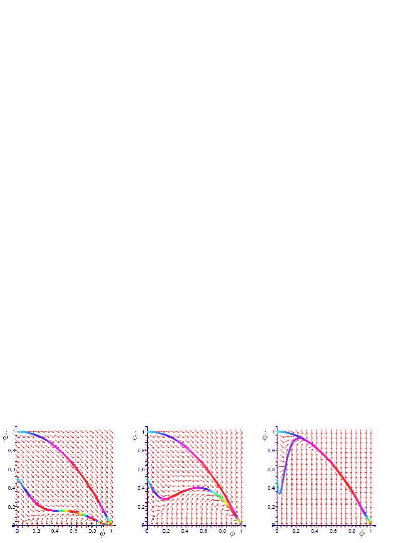
Figure 6: The phase portraits at $m_{p}^{2}\leqslant 1/2$. Thick lines strokes depict solutions with the initial conditions $\dot{\phi}(0)=1/2$ and $\dot{\phi}(0)=1$.

Thus both behavior of the first corrections and phase portraits show that the obtained exact solution is stable for $m_{p}^{2}\leqslant 1/2$.

4.2 Variation of the form of the potential

In this subsection we investigate an influence of variation of the coefficients in the second summand of the potential (16) on the behavior of solutions to system (5). Consider a dynamics of system (5) with the potential

$$\tilde{V}(\phi)=\frac{1}{2}\left(1-\phi^{2}\right)^{2}+\frac{y}{12m_{p}^{2}}\phi^{2}\left(3-\phi^{2}\right)^{2}.$$

Parameter $y$ is introduced so that the points $\phi=\pm 1$ remain the extrema of the potential. Note, that up to a constant shift and an overall factor multiplication this is the only possible modification of an even potential (16), which leaves the points $\phi=\pm 1$ to be extrema. Equation (7) differs from the kink equation of motion (11) by the friction like term and an extra proportional to $1/m_{p}^{2}$ term in the potential. Parameter $y$ enables us to separate the effects of the friction and an extra term in the potential and to answer the question which one provides the stability of solution.

To analyze stability it is convenient to plot phase portraits for different values of parameters $m_{p}$ and $y$ and to render them in a table as it is done in Figs. 7 and 8. Guided by the plotted phase portraits and an analysis performed in Sections 3 and 4, we conclude the stabilization of solutions is due to an extra term in the potential. Namely, the obtained solution is attractive one for $m_{p}^{2}/y\leqslant 1/2$ irrespectively the numeric factor in the friction term.

$\qquad\qquad\qquad y=0.2$ $y=1$ $y=1.8\qquad\qquad\qquad\quad$

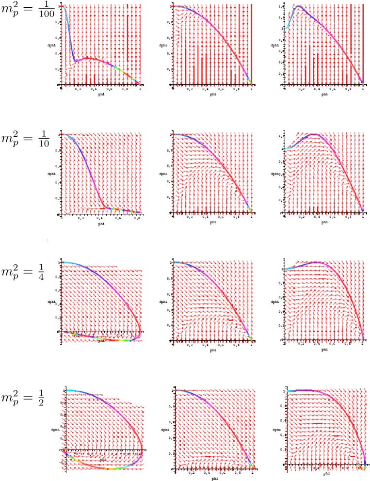
Figure 7: Phase portraits for $m_{p}^{2}\leqslant 1/2$ and various $y$.

$\qquad\qquad\quad y=0.2$ $y=1$ $y=1.8\qquad\qquad\qquad$

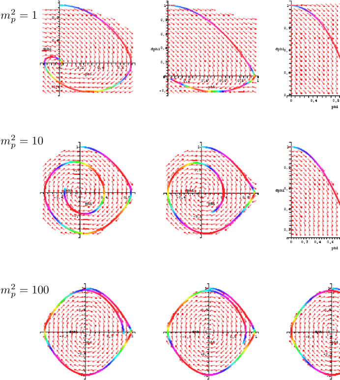
Figure 8: Phase portraits for $m_{p}^{2}>1/2$ and various $y$.

5 Conclusion

In the present paper we have performed an analysis of an exactly solvable model of accelerating expanded Universe dominated by the dark energy. The state parameter of the model in the consideration is always less than $-1$ and tends to $-1$ when $t\to\infty$. Such a behavior of the state parameter leads to an absence of the Big Rip singularity in our model. This kind of singularity does exist in the model with a constant $w<-1$. Note, that these properties of the state parameter are kept after including in our model an interaction with the cold dark matter [65]. It is shown also in this paper that our solution is stable with respect to small fluctuations of initial data when $m_{p}^{2}\leqslant 1/2$ and small fluctuations of the form of the potential. The simplest way to yield an exactly solvable model with $w$ crossing the cosmological constant barrier $w=-1$ consists in an inclusion of an additional scalar field [66].

Authors are grateful to A.E. Pukhov and I.V. Volovich for useful discussions. The work is supported in part by RFBR grant 05-01-00758, I.Ya. and A.K. are supported in part by INTAS grant 03-51-6346 and Russian President’s grant NSh-2052.2003.1, the work of S.V. is financially supported in part by Russian President’s grant NSh-1685.2003.2 and grant of the scientific program “Universities of Russia” 02.02.503.

Appendix. Cosmo-phantom versus 5-dimensional gravity models

Our model as whole and system (5) in particular are in close analogy with models considered in brane-world scenarios. Let us compare system (5) with the system of the Einstein equations in the model of gravity interacting with a single scalar field in five-dimensional space-time [63, 67]. The action is

$$\tilde{S}=\int d^{4}xdr\sqrt{|\det\,\tilde{g}_{\mu\nu}|}\left(\frac{\tilde{R}}{4}-\frac{1}{2}\tilde{g}^{\mu\nu}\partial_{\mu}\tilde{\phi}\partial_{\nu}\tilde{\phi}-V(\tilde{\phi})\right),$$

where $\tilde{g}_{\mu\nu}$ is defined as follows

$$d\tilde{s}^{2}=e^{2A(r)}(-dx_{0}^{2}+dx_{1}^{2}+dx_{2}^{2}+dx_{3}^{2})+dr^{2}.$$

Assuming the scalar field depends only on $r$, the independent equations of motion are

$$\tilde{H}^{\prime}=-\frac{8}{9}(\tilde{\phi}^{\prime})^{2},$$ (25)

$$3\tilde{H}^{2}=-\frac{16}{9}\left(V(\tilde{\phi})-\frac{1}{2}(\tilde{\phi}^{\prime})^{2}\right),$$ (26)

where $\tilde{H}\equiv 4A^{\prime}/3\equiv\frac{4}{3}\frac{\mathrm{d}A}{\mathrm{d}r}$ and $\tilde{\phi}^{\prime}\equiv\frac{\mathrm{d}\tilde{\phi}}{\mathrm{d}r}$. These equations correspond to (5) with $m_{p}^{2}=-9/16$. Surely, such a choice of the $m_{p}^{2}$ coupling is not physical, but we see that the method described in [63] to transform (5) into the first order differential equation works in our case as well, i.e. mathematical method, which simplifies (25) and (26), does not depend on a value or sign of $m_{p}^{2}$.

References

- [1] S.J. Perlmutter et al., Measurements of Omega and Lambda from High-Redshift Supernovae, Astroph. J. 517 (1999) 565; astro-ph/9812133.
- [2] A. Riess et al., Type Ia Supernova Discoveries at From the Hubble Space Telescope: Evidence for Past Deceleration and Constraints on Dark Energy Evolution, Astrophys. J. 607 (2004) 665; astro-ph/0402512.
- [3] A. Riess et al., Observational Evidence from Supernovae for an Accelerating Universe and a Cosmological Constant, Astron. J. 116 (1998) 1009; astro-ph/9805201.
- [4] D.N. Spergel et al., First Year Wilkinson Microwave Anisotropy Probe (WMAP) Observations: Determination of Cosmological Parameters, Astroph. J. Suppl. 148 (2003) 175; astro-ph/0302209.
- [5] V. Sahni, A.A. Starobinsky, The Case for a Positive Cosmological Lambda-term, Int. J. Mod. Phys. D9 (2000) 373; astro-ph/9904398; V. Sahni, Dark Matter and Dark Energy, astro-ph/0403324.
- [6] P. Frampton, Dark energy — a pedagogic review, astro-ph/0409166.
- [7] T. Padmanabhan, Cosmological Constant — the Weight of the Vacuum, Phys. Rept. 380 (2003) 235; hep-th/0212290.
- [8] R.R. Caldwell, Dark Energy, Physics World 17, No. 5 (2004) 37.
- [9] R. Bean, S. Carroll, M. Trodden, Insights into dark energy: interplay between theory and observation, astro-ph/0510059; T. Padmanabhan, Darker side of the Universe, astro-ph/0510492.
- [10] R.A. Knop et al., New constraints on , , and from an independent set of eleven high — redshift supernovae observed with HST, Astrophys.J. 598 (2003) 102, astro-ph/0309368.
- [11] M. Tegmark et al., The 3-d power spectrum of galaxies from the SDSS, Astroph. J. 606 (2004) 702; astro-ph/0310723.
- [12] S. Hannestad, E. Mortsell, Probing the dark side: Constraints on the dark energy equation of state from CMB, large scale structure and Type Ia supernovae, Phys. Rev. D66 (2002) 063508; astro-ph/0205096; S. Hannestad, E. Mortsell, Cosmological constraints on the dark energy equation of state and its evolution, JCAP 0409 (2004) 001; astro-ph/0407259.
- [13] A. Melchiorri, L. Mersini, C.J. Odman, M. Trodden, The State of the Dark Energy Equation of State, Phys. Rev. D68 (2003) 043509; astro-ph/0211522.
- [14] J.L. Tonry et al., Cosmological Results from High-z Supernovae, Astrophys. J. 594 (2003) 1; astro-ph/0305008.
- [15] C. Wetterich, Cosmology and the Fate of Dilatation Symmetry, Nucl. Phys. B302 (1988) 668.
- [16] B. Ratra, P.J.E. Peebles, Cosmology With A Time Variable Cosmological ’Constant’, Astrophys. J. 325 (1988) L17.
- [17] R.R. Caldwell, R. Dave, P.J. Steinhardt, Cosmological Imprint of an Energy Component with General Equation of State, Phys. Rev. Lett. 80 (1998) 1582; astro-ph/9708069.
- [18] L. Wang, R.R. Caldwell, J.P. Ostriker, P.J. Steinhardt, Cosmic Concordance and Quintessence, Astrophys. J. 530 (2000) 17; astro-ph/9901388.
- [19] C. Armendariz-Picon, V. Mukhanov, P.J. Steinhardt, A Dynamical Solution to the Problem of a Small Cosmological Constant and Late-time Cosmic Acceleration, Phys. Rev. Lett. 85 (2000) 4438; astro-ph/0004134; C. Armendariz-Picon, V. Mukhanov, P.J. Steinhardt, Essentials of k-essence, Phys. Rev. D63 (2001) 103510; astro-ph/0006373.
- [20] G.W. Gibbons, Thoughts on Tachyon Cosmology, Class. Quant. Grav. 20 (2003) S321; hep-th/0301117.
- [21] A. Sen, Tachyon Dynamics in Open String Theory, hep-th/0410103.
- [22] E.J. Copeland, M.R. Garousi, M. Sami, Sh. Tsujikawa, What is needed of a tachyon if it is to be the dark energy?, Phys. Rev. D71 (2005) 043003; hep-th/0411192.
- [23] L.B. Okun’. Leptons and quarks. Amsterdam, North-Holland, 1982. Second edition: Moscow, ”Nauka”, 1990, {in Russian}.
- [24] R.R. Caldwell, A Phantom Menace? Cosmological consequences of a dark energy component with super-negative equation of state, Phys. Lett. B545 (2002) 23; astro-ph/9908168.
- [25] B. McInnes, The dS/CFT Correspondence and the Big Smash, JHEP 0208 (2002) 029; hep-th/0112066.
- [26] R.R. Caldwell, M. Kamionkowski, N.N. Weinberg, Phantom Energy and Cosmic Doomsday, Phys. Rev. Lett. 91 (2003) 071301; astro-ph/0302506.
- [27] S. Nesseris, L. Perivolaropoulos, The Fate of Bound Systems in Phantom and Quintessence Cosmologies, Phys. Rev. D70 (2004) 123529; astro-ph/0410309.
- [28] S.M. Carroll, M. Hoffman, M. Trodden, Can the dark energy equation-of-state parameter be less than ?, Phys. Rev. D68 (2003) 023509; astro-ph/0301273.
- [29] J.M. Cline, S. Jeon, G.D. Moore, The phantom menaced: constraints on low-energy effective ghosts, Phys. Rev. D70 (2004) 043543; hep-ph/0311312.
- [30] S.D.H. Hsu, A. Jenkins, M.B. Wise, Gradient instability for , Phys. Lett. B597 (2004) 270; astro-ph/0406043.
- [31] V.K. Onemli, R.P. Woodard, Super-Acceleration from Massless, Minimally Coupled , Class. Quant. Grav. 19 (2002) 4607; gr-qc/0204065; V.K. Onemli, R.P. Woodard, Quantum effects can render on cosmological scales, Phys. Rev. D70 (2004) 107301; gr-qc/0406098.
- [32] U. Alam, V. Sahni, A.A. Starobinsky, The case for dynamical dark energy revisited, JCAP 0406 (2004) 008; astro-ph/0403687.
- [33] T. Padmanabhan, Accelerated expansion of the universe driven by tachyonic matter, Phys. Rev. D66 (2002) 021301; hep-th/0204150;
- [34] T. Padmanabhan, T. Roy Choudhury, Can the clustered dark matter and the smooth dark energy arise from the same scalar field?, Phys. Rev. D66 (2002) 081301; hep-th/0205055.
- [35] A. Melchiorri, L. Mersini, C.J. Odman, M. Trodden, The State of the Dark Energy Equation of State, Phys. Rev. D68 (2003) 043509; astro-ph/0211522.
- [36] Bo Feng, Xiulian Wang, Xinmin Zhang, Dark Energy Constraints from the Cosmic Age and Supernova, Phys. Lett. B607 (2005) 35; astro-ph/0404224; Bo Feng, Mingzhe Li, Yun-Song Piao, Xinmin Zhang, Oscillating Quintom and the Recurrent Universe, astro-ph/0407432.
- [37] S. Nojiri, S. Odintsov, The final state and thermodynamics of dark energy universe, Phys. Rev. D70 (2004) 103522; hep-th/0408170.
- [38] W. Fang, H.Q. Lu, Z.G. Huang, K.F. Zhang, Phantom Cosmology with Born-Infeld Type Scalar Field, hep-th/0409080.
- [39] Jian-gang Hao, Xin-zhou Li, Attractor Solution of Phantom Field, Phys. Rev. D67 (2003) 107303; gr-qc/0302100.
- [40] P. Singh, M. Sami, N. Dadhich, Cosmological Dynamics of Phantom Field, Phys. Rev. D68 (2003) 023522; hep-th/0305110.
- [41] Rong-Gen Cai, Anzhong Wang, Cosmology with Interaction between Phantom Dark Energy and Dark Matter and the Coincidence Problem, JCAP 0503 (2005) 002; hep-th/0411025.
- [42] Zong-Kuan Guo, Yuan-Zhong Zhang, Interacting Phantom Energy, astro-ph/0411524.
- [43] S.M. Carroll, A. De Felice, M. Trodden, Can we be tricked into thinking that is less than ?, Phys. Rev. D71 (2005) 023525; astro-ph/0408081.
- [44] I.Ya. Aref’eva, Nonlocal String Tachyon as a Model for Cosmological Dark Energy, astro-ph/0410443.
- [45] M. Kaplinghat, S. Bridle, Testing for a Super-Acceleration Phase of the Universe, Phys. Rev. D71 (2005) 123003; astro-ph/0312430.
- [46] C. Csaki, N. Kaloper, J. Terning, Exorcising , Annals Phys. 317 (2005) 410; astro-ph/0409596; C. Csaki, N. Kaloper, J. Terning, Dimming Supernovae without Cosmic Acceleration, Phys. Rev. Lett. 88 (2002) 161302; hep-ph/0111311.
- [47] A. Vikman, Can dark energy evolve to the Phantom?, Phys. Rev. D71 (2005) 023515; astro-ph/0407107.
- [48] A.A. Andrianov, F. Cannata, A.Y. Kamenshchik, Smooth dynamical (de)-phantomization of a scalar field in simple cosmological models, Phys. Rev. D72 (2005) 043531; gr-qc/0505087.
- [49] A.A. Starobinsky, J. Yokoyama, Equilibrium State of a Massless Self-Interacting Scalar Field in the De Sitter Background, Phys. Rev. D50 (1994) 6357; astro-ph/9407016.
- [50] C. Deffayet, G. Dvali, G. Gabadadze, Accelerated Universe from Gravity Leaking to Extra Dimensions, Phys. Rev. D65 (2002) 044023; astro-ph/0105068; R. Kallosh, A.Linde, M-theory, Cosmological Constant and Anthropic Principle, Phys. Rev. D67 (2003) 023510; hep-th/0208157; Sh. Mukohyama, L. Randall, A dynamical approach to the cosmological constant, Phys. Rev. Lett. 92 (2004) 211302; hep-th/0306108; V. Sahni, Y. Shtanov, Brane World Models of Dark Energy, JCAP 0311 (2003) 014; astro-ph/0202346; Ph. Brax, C. van de Bruck, A.-C. Davis, Brane world cosmology, Rept. Prog. Phys. 67 (2004) 2183; hep-th/0404011; Th.N. Tomaras, Brane-world evolution with brane-bulk energy exchange, hep-th/0404142; E.J. Copeland, M.R. Garousi, M. Sami, Sh. Tsujikawa, What is needed of a tachyon if it is to be the dark energy?, Phys. Rev. D71 (2005) 043003; hep-th/0411192.
- [51] I.Ya. Arefeva, D.M. Belov, A.S. Koshelev, P.B. Medvedev, Tahyon Condensation in the Cubic Superstring Field Theory, Nucl. Phys B638 (2002) 3; hep-th/0011117.
- [52] K. Ohmori, A Review on Tachyon Condensation in Open String Field Theories, hep-th/0102085; I.Ya. Aref’eva, D.M. Belov, A.A. Giryavets, A.S. Koshelev, P.B. Medvedev, Noncommutative Field Theories and (Super)String Field Theories, hep-th/0111208; W. Taylor, Lectures on D-branes, tachyon condensation and string field theory, hep-th/0301094.
- [53] B. McInnes, The Phantom Divide in String Gas Cosmology, Nucl. Phys. B718 (2005) 55; hep-th/0502209.
- [54] E. Witten, Noncommutative Geometry And String Field Theory, Nucl. Phys. B268 (1986) 253.
- [55] I.Ya. Aref’eva, P.B. Medvedev, A.P. Zubarev, Background formalism for superstring field theory, Nucl. Phys. B341 (1990) 464.
- [56] C.R. Preitschopf, C.B. Thorn, S.A. Yost, Superstring Field Theory, Nucl. Phys. B337 (1990) 363.
- [57] N. Moeller, B. Zwiebach, Dynamics with Infinitely Many Time Derivatives and Rolling Tachyons, JHEP 0210 (2002) 034; hep-th/0207107
- [58] I.Ya. Aref’eva, L.V. Joukovskaya, A.S. Koshelev, Time Evolution in Superstring Field Theory on non-BPS brane. Rolling Tachyon and Energy-Momentum Conservation, JHEP 0309 (2003) 012; hep-th/0301137.
- [59] Ya.I. Volovich, Numerical study of nonlinear equations with infinite number of derivatives, J. Phys. A36 (2003) 8685; math-ph/0301028.
- [60] V.S. Vladimirov, I.V. Volovich, E.I. Zelenov, p-adic Analysis and Mathematical Physics, WSP, Singapore, 1994.
- [61] V.S. Vladimirov, Ya.I. Volovich, Nonlinear Dynamics Equation in p-Adic String Theory, Theor. Math. Phys., 138 (2004) 297; math-ph/0306018.
- [62] L. Brekke, P.G.O. Freund, M. Olson, E. Witten, Nonarchimedean String Dynamics, Nucl.Phys. B302 (1988) 365.
- [63] O. DeWolfe, D.Z. Freedman, S.S. Gubser, A. Karch, Modeling the fifth dimension with scalars and gravity, Phys. Rev. D62 (2000) 046008; hep-th/9909134.
- [64] S.Yu. Vernov, From the Laurent-series Solutions of Nonintegrable Systems to the Elliptic Solutions of them, astro-ph/0502356.
- [65] I.Ya. Aref’eva, A.S. Koshelev, S.Yu. Vernov, Stringy Dark Energy Model with Cold Dark Matter, Phys. Lett. B628 (2005) 1; astro-ph/0505605.
- [66] I.Ya. Aref’eva, A.S. Koshelev, S.Yu. Vernov, Crossing of the Barrier by D3-brane Dark Energy Model, Phys. Rev. D72 (2005) 064017; astro-ph/0507067.
- [67] M. Gremm, Four-dimensional gravity on a thick domain wall, Phys. Lett. B478 (2000) 434; hep-th/9912060; M. Gremm, Thick domain walls and singular spaces, Phys. Rev. D62 (2000) 044017; hep-th/0002040.