Probing Quantum Decoherence in Atmospheric Neutrino Oscillations with a Neutrino Telescope

Abstract

Quantum decoherence, the evolution of pure states into mixed states, may be a feature of quantum gravity. In this paper, we show how these effects can be modelled for atmospheric neutrinos and illustrate how the standard oscillation picture is modified. We examine how neutrino telescopes, such as ANTARES, are able to place upper bounds on these quantum decoherence effects.

1 Introduction

Quantum field theory and general relativity are supremely successful theories, both having been experimentally verified to great accuracy. However, these two theories are fundamentally incompatible: general relativity is non-renormalizable as a quantum field theory. Many candidate theories of quantum gravity exist in the literature, but there is as yet no consensus as to which will provide the final fundamental theory. For a recent review of the current state of play, see [1]. Quantum gravity becomes particularly important in two realms of physics: the very early universe (prior to the Planck time, $10^{-43}$ s); and in black holes, when gravitational fields are strong but quantum effects cannot be ignored.

There are two different approaches to uncovering the theory of quantum gravity: firstly, there is the ‘top down’ method, which involves writing a theory down and then attempting to see if the theory can make any physical predictions which are testable. The second, which is the method embraced here, is the ‘bottom up’ method, in which we analyze experimental data and attempt to fit the data to various phenomenological models (for a recent review, see, for example, [2]). This way, we may narrow down the number of models until, eventually, a single theory emerges, which is consistent with experiment. There are various ways in which quantum gravity may alter fundamental physics; the final theory will no doubt include highly unexpected effects on basic physical principles. Here we are concerned only with one such mechanism: the influence of quantum gravity on standard quantum mechanical time-evolution.

Naively, one might expect that quantum gravity is beyond the reach of experimental physics, since its relevant energy scale is the Planck energy, approximately $10^{19}$ GeV. However, recent theoretical models coming from string theory suggest that the energy scale of quantum gravity may be as low as a few TeV [3]. Moreover, even with more conservative estimates of the quantum gravity energy scale, comparatively low energy physics may be sensitive to quantum gravity effects, for example, through quantum-gravity induced modifications of quantum mechanics resulting in quantum decoherence [4].

In this article we are concerned with one such low-energy system: atmospheric neutrinos. This is a comparatively simple quantum system, which lends itself to an analysis of quantum decoherence effects. There is already a body of work on the theoretical modelling of quantum decoherence effects on neutrino oscillations [5, 6, 7, 8, 9]. However, the only analysis of decoherence effects in experimental data relating to $\nu_{\mu}\rightarrow\nu_{\tau}$ oscillations available in the literature to date is for Super-Kamiokande and K2K data [10, 11, 12]. An initial analysis [10] was able to put bounds on quantum decoherence effects in a simple model. Subsequently, a detailed analysis of the same simple model [11] found that quantum decoherence effects were slightly disfavoured compared with the standard oscillation scenario, but that they could not be completely ruled out. Further experimental work is therefore needed, and here we shall study the sensitivity of the ANTARES neutrino telescope [13] to these quantum decoherence effects in atmospheric neutrino oscillations. Although neutrino telescopes such as ANTARES are primarily designed for the detection and study of neutrinos of astrophysical and cosmological origin, atmospheric neutrinos form the most important background to such sources and are likely to provide the first physics results.

As well as the simple model considered in Refs. [10, 11], in this paper we shall study models which are more exotic than those considered previously, as they include effects such as non-conservation of energy (within the neutrino system). Furthermore, while these models have been studied theoretically in the literature [5, 6, 7, 8, 9], they have not been experimentally tested. It should be emphasized that such quantum decoherence is not the only possible effect of quantum gravity on neutrinos [14]. For example, quantum gravity is expected to change the energy dependence of the oscillation length [15], and also alter the dispersion relation [16], leading to observable effects [17]. We shall also briefly discuss other, non-quantum gravity, possible corrections to atmospheric neutrino oscillations and how they relate to our models here, as well as comparing our results on quantum decoherence parameters with those coming from other experimental (i.e. non-neutrino) systems (see, for example, [18, 19]). Finally, although our simulations are specific to ANTARES, we anticipate that other high energy neutrino experiments such as AMANDA [20], IceCube [21] and NESTOR [22], may well be able to probe these effects.

Given the high energy and long path-length of atmospheric neutrinos studied by ANTARES, this study is complementary to “long-baseline” neutrino oscillation experiments. As well as the analysis of K2K data [11], a related analysis of KAMLAND data has also been performed in [23]. In both cases decoherence is disfavoured over the standard oscillation picture. The potential for bounding quantum decoherence and other damping signatures in future reactor experiments, such as MINOS [24] and OPERA [25], is discussed in [26].

The outline of this paper is as follows. In section 2, we discuss how quantum gravity may be expected to modify quantum mechanics, before applying the formalism developed to atmospheric neutrino oscillations in section 3. We study in detail some specific models of quantum decoherence in section 4, and describe the results of ANTARES sensitivity simulations for these models in section 5. The projected ANTARES sensitivities are compared with results from other experiments (both neutrino and non-neutrino) in section 6, and we briefly discuss other possible corrections to atmospheric neutrino oscillations in section 7. Finally, our conclusions are presented in section 8. Unless otherwise stated, we use units in which $c=\hbar=1$.

2 Quantum gravity induced modifications of quantum mechanics

In quantum gravity, space-time is expected to adopt a ‘foamy’ structure [27]: tiny black holes form out of the vacuum (in the same way that quantum particles can be formed out of the vacuum). These will be very short-lived, evaporating quickly by Hawking radiation [28]. Each microscopic black hole may induce variations in the standard time-evolution of quantum mechanics, as an initially pure quantum state (describing the space-time before the formation of the black hole) can evolve to a mixed quantum state (describing the Hawking radiation left after the black hole has evaporated). In particular, in quantum gravity it is no longer necessarily the case that pure states cannot evolve to mixed states.

In order to describe this process, Hawking suggested a quantum gravitational modification of quantum mechanics [29], which is based on the density matrix formalism. An initial quantum state is described by a density matrix $\rho_{in}$, and this state then evolves to a final state described by a density matrix $\rho_{out}$. The two density matrices are related by

$$\rho_{out}=\$\rho_{in},$$

where $\$$ is an operator known as the super-scattering operator. In ordinary quantum mechanics, the super-scattering operator can be factorized as

$$\$=\mathcal{S}\mathcal{S}^{{\dagger}},$$ (1)

where ${\mathcal{S}}$ is the usual $S$-matrix. In this case, a pure initial state always leads to a pure final state. However, in quantum gravity it is no longer necessarily the case that the super-scattering matrix can be factorized as in equation (1), and, if it cannot, then the evolution from pure state to mixed state is allowed. The disadvantage of this approach is that it requires the construction of asymptotic “in” and “out” states.

Therefore, here we will take an alternative approach, which is more useful for our application to atmospheric neutrino oscillations, allowing the evolution of pure to mixed states by modifying the differential equation describing the time-evolution of the density matrix $\rho$ [4]. In standard quantum mechanics this differential equation takes the form

$$\dot{\rho}=-i[H,\rho],$$

and could be modified by quantum gravity to the equation [4]

$$\dot{\rho}=-i[H,\rho]+\delta\!\!\,\!\!/H\rho.$$ (2)

In the above equations, $H$ is the Hamiltonian of the system, $\delta\!\!\,\!\!/H$ is the most general linear extension which maps hermitian matrices to hermitian matrices and the dot denotes differentiation with respect to time. Various conditions need to be imposed on $\delta\!\!\,\!\!/H$ to ensure that probability is still conserved and that ${\rm{Tr}}\rho^{2}$ is never greater than unity [4]. These conditions will be implemented in the next section when we apply this approach to atmospheric neutrinos. However, the precise form of $\delta\!\!\,\!\!/H$ would need to come from a complete, final, theory of quantum gravity. In this paper we take a phenomenological approach, modelling $\delta\!\!\,\!\!/H$ in a manner independent of its origin in quantum gravity. Ultimately one may hope that experimental observations may be able to constrain the form of $\delta\!\!\,\!\!/H$ and hence its theoretical origin.

One form of $\delta\!\!\,\!\!/H$ which is frequently employed in the literature is the Lindblad form [30]

$$\delta\!\!\,\!\!/H\rho=\sum_{n}\left[D_{n},\left[D_{n},\rho\right]\right],$$ (3)

where the $D_{n}$ are self-adjoint operators which commute with the Hamiltonian of the theory. Such modifications of standard quantum-mechanical time evolution have been widely studied, both as a solution to the quantum measurement problem [31] and for decoherence due to the interaction with an environment [32]. In recent work in discrete quantum gravity, it has been shown that $\delta\!\!\,\!\!/H$ has the Lindblad form with a single operator $D$ which is proportional to the Hamiltonian $H$ [33]. However, it should be emphasized that this is not the only possible approach to quantum gravity, and that other formulations indicate that in general $\delta\!\!\>\!\!/H$ does not have the Lindblad form. This is the reason for our more general set-up in this paper.

Modifications of quantum mechanics (whether from quantum gravity or other origins) of the form (2) are often known as quantum decoherence effects as they emerge from dissipative interactions with an environment (of which space-time foam is just one example), and allow transitions from pure to mixed quantum states (i.e. a loss of coherence). Such effects have been studied in quantum systems other than atmospheric neutrinos, for example, the neutral kaon system, for which there exists an extensive literature (see, for example, [18, 19]).

It should be stressed that although our primary motivation for studying quantum decoherence is from quantum gravity, in fact our modelling in the subsequent sections is independent of the source of the quantum decoherence. Furthermore, Ohlsson [34] has discussed how Gaussian uncertainties in the neutrino energy and path length, when averaged over, can lead to modifications of the standard neutrino oscillation probability which are similar in form to those coming from quantum decoherence, and which are therefore included in our analysis. See also [35] for further discussion of these effects.

3 Quantum decoherence modifications of atmospheric neutrino oscillations

We now consider how quantum gravity induced modifications of quantum mechanics, as outlined in the previous section, may affect atmospheric neutrino oscillations. The quantum system of interest is then simply made up of muon and tau neutrinos. The mathematical modelling of quantum decoherence effects in this system is not dissimilar to that for the neutral kaon system [4, 18]. In this paper we will assume that quantum decoherece affects neutrinos and anti-neutrinos in the same way, and do not consider the possibility that quantum decoherence may appear only in the anti-neutrino sector [36].

In order to implement equation (2) for the system of atmospheric muon and tau neutrinos, we need to represent the matrices $H$ and $\rho$ in terms of a specific basis which comprises the standard Pauli matrices $\sigma_{i}$. We may, therefore, write the density matrix, Hamiltonian and additional term $\delta\!\!\>\!\!/H$ in terms of the Pauli matrices as

$$\rho=\frac{1}{2}\rho_{\mu}\sigma_{\mu};\quad\quad H=\frac{1}{2}h_{\nu}\sigma_{\nu};\quad\quad\delta\!\!\>\!\!/H=\frac{1}{2}h^{\prime}_{\kappa}\sigma_{\kappa};$$

where the Greek indices run from 0 to 3, and a summation over repeated indices is understood. Similarly decomposing the time derivative of the density matrix,

$${\dot{\rho}}=\frac{1}{2}{\dot{\rho}}_{\mu}\sigma_{\mu},$$

where, using equation (2):

$$\dot{\rho}_{\mu}=(h_{\mu\nu}+h^{\prime}_{\mu\nu})\rho_{\nu}.$$ (4)

Here, $h$ represents the standard atmospheric neutrino oscillations and $h^{\prime}$ the quantum decoherence effects. In order to preserve unitarity, the first row and column of the matrix $h^{\prime}$ must vanish; the fact that ${\rm{Tr}}\rho^{2}$ can never exceed unity means that $h^{\prime}$ must be negative semi-definite [4]. The most general form of $h^{\prime}$ is therefore given by

$$h^{\prime}=-2\left(\begin{array}[]{cccc}0&0&0&0\\ 0&a&b&d\\ 0&b&\alpha&\beta\\ 0&d&\beta&\delta\\ \end{array}\right);$$ (5)

where $a$, $b$, $d$, $\alpha$, $\beta$ and $\delta$ are real constants parameterizing the quantum decoherence effects.

Particularly with regard to quantum decoherence induced by space-time foam (see section 2), it is not clear exactly what assumptions about the time-evolution matrix $h^{\prime}$ are reasonable, for example, it may no longer be the case that energy is conserved within the neutrino system, as energy may be lost to the environment of space-time foam. The first observation is that $h^{\prime}$ has non-zero entries in the final row and column ($d$, $\beta$ and $\delta$), which correspond to terms which violate energy conservation [4]. The matrix $h^{\prime}$ can be further simplified by making additional assumptions. For example, since the eigenvalues of the density matrix $\rho$ correspond to probabilities, we require that these are positive (this is known as simple positivity). However, we can make a much stronger assumption known as complete positivity, discussed in [5]. It arises in the quantum mechanics of open systems, and ensures the positivity of the density matrix describing a much larger system, in which the neutrinos are coupled to an external system. Complete positivity is a strong assumption, favoured by mathematicians because it is a powerful tool in proving theorems related to quantum decoherence. For the matrix $h^{\prime}$, assuming complete positivity leads to a number of inequalities on the quantum decoherence parameters [5], and assuming both complete positivity and energy conservation within the neutrino system means that $a=\alpha$ and all other quantum decoherence parameters must vanish [5] (which gives the Lindblad form (3)). It is this simplified model which has been most studied in the literature to date [10, 11]. However, in this paper we wish to consider not only this simplified model but other more general models of quantum decoherence which do not necessarily satisfy complete positivity or energy conservation.

Substituting (5) into (4), and incorporating the standard atmospheric neutrino oscillations in the matrix $h$ (4), we obtain the following differential equations for the time-evolution of the components of the density matrix:

$$\dot{\rho}_{0} = 0;$$

$$\dot{\rho}_{1} = -2a\rho_{1}-2\left(b-\frac{\Delta m^{2}}{4E}\right)\rho_{2}-2d\rho_{3};$$

$$\dot{\rho}_{2} = -2\left(b+\frac{\Delta m^{2}}{4E}\right)\rho_{1}-2\alpha\rho_{2}-2\beta\rho_{3};$$

$$\dot{\rho}_{3} = -2d\rho_{1}-2\beta\rho_{2}-2\delta\rho_{3};$$ (6)

where $\Delta m^{2}$ is the usual difference in squared masses of the neutrino mass eigenstates, and $E$ is the neutrino energy.

By integrating the differential equations (6) with suitable initial conditions, the probability for a muon neutrino to oscillate into a tau neutrino can be calculated. In general, this probability has the form [5]:

$$P\left[\nu_{\mu}\rightarrow\nu_{\tau}\right] = \frac{1}{2}\left\{1-\cos^{2}(2\theta)M_{33}(E,L)-\sin^{2}(2\theta)M_{11}(E,L)\right.$$ (7)

$$\left.-\frac{1}{2}\sin 4\theta\left[M_{13}(E,L)+M_{31}(E,L)\right]\right\},$$

where the functions $M_{11}(E,L)$, $M_{33}(E,L)$, $M_{13}(E,L)$ and $M_{31}(E,L)$ are elements of the matrix $M(E,L)$ which is defined as

$$M(E,L)=\exp\left[-2{\mathcal{H}}(E)L\right],$$

where

$${\mathcal{H}}(E)=\left(\begin{array}[]{ccc}a&b-\frac{\Delta m^{2}}{4E}&d\\ b+\frac{\Delta m^{2}}{4E}&\alpha&\beta\\ d&\beta&\delta\end{array}\right).$$

In general there is no simple closed form expression for the elements of the matrix $M(E,L)$. Here we shall study various special cases in which there will be closed form functions of the new parameters appearing in the probability (7). For each model, we consider three possible ways in which the quantum decoherence parameters can depend on the energy $E$ of the neutrinos (we shall assume that where there are two or more quantum decoherence parameters, they have the same energy dependence):

1. Firstly, the simplest model is to suppose that the quantum decoherence parameters are constants, and have no energy dependence. In this case we write

   $$\alpha=\frac{1}{2}\gamma_{\alpha},$$

   with similar expressions for the other quantum decoherence parameters.

2. Secondly, we consider the situation in which the quantum decoherence parameters are inversely proportional to the energy $E$, which leads to probabilities which are Lorentz invariant. We define the constants of proportionality $\mu_{\alpha}$ etc. according to the equation:

   $$\alpha=\frac{\mu^{2}_{\alpha}}{4E}.$$

   This energy dependence has received the most attention to date in the literature [10, 11]. We should comment that Lorentz invariance is not necessarily expected to hold exactly in quantum gravity [16].

3. Finally, we study a model suggested in reference [4], and which arises in some semi-classical calculations of decoherence phenomena in black hole and recoiling D-brane geometries [37], namely that the quantum decoherence parameters are proportional to the energy squared, so that the quantum decoherence parameters are given by expressions of the form

   $$\alpha=\frac{1}{2}\kappa_{\alpha}E^{2},$$

   where $\kappa_{\alpha}$ is a constant. This energy dependence also arises from discrete quantum gravity [33], where the operator $D$ in the Lindblad form (3) is proportional to the Hamiltonian. On dimensional grounds, the constant of proportionality $\kappa$ contains a factor of $1/M_{P}$, where $M_{P}$ is the Planck mass, $10^{28}$ eV. This suppression of quantum gravity effects by a single power of the Planck mass is naively unexpected (as it corresponds to a dimension-5, non-renormalizable operator in the theory, see, for example [38]). One would instead expect quantum gravity effects to be suppressed by the Planck mass squared.

We should also point out that an alternative energy dependence, namely that quantum decoherence parameters are proportional to

$$\frac{\left(\Delta m^{2}\right)^{2}}{E^{2}}$$

has been suggested from $D$-brane interactions in non-critical string theory [14, 39]. However, we have not been able to derive any meaningful results for this energy dependence, in accordance with the observation in [14] that it is unlikely that current, or even planned, experiments will be able to probe this energy dependence.

To see how quantum decoherence affects atmospheric neutrino oscillations, we now compare the oscillation probabilities. Although the oscillation probabilities are unobservable directly, they nonetheless provide insight into the underlying physics behind observable neutrino behaviour. Firstly, the standard atmospheric neutrino oscillation probability is given by

$$P[\nu_{\mu}\rightarrow\nu_{\tau}]=\frac{1}{2}\left[1-\cos\left(6.604\times 10^{-3}\frac{L}{E}\right)\right];$$ (8)

where we have restored the constants $c$ and $\hbar$ and the neutrino energy $E$ is measured in GeV with the path length $L$ being measured in km. In equation (8), we have taken $\Delta m^{2}$ and $\sin^{2}(2\theta)$ to have their best-fit values [11]

$$\Delta m^{2}=2.6\times 10^{-3}{\mbox{eV${}^{2}$}};\qquad\sin^{2}(2\theta)=1.$$ (9)

The oscillation probability (8) is plotted in figure 1 as a function of path length $L$, for fixed neutrino energy $E$ equal to 1 GeV and 200 GeV, and in figure 2 as a function of neutrino energy $E$ for fixed path length $L$ equal to 10000 km.

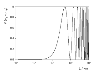
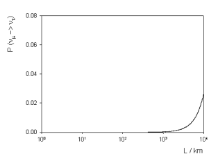
Figure 1: Standard atmospheric neutrino oscillation probability (8) as a function of path length $L$ (measured in km), for fixed neutrino energy $E$ equal to 1 GeV (top) and 200 GeV (bottom).

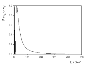
Figure 2: Standard atmospheric neutrino oscillation probability (8) as a function of neutrino energy $E$ (measured in GeV), for fixed path length equal to 10000 km.

Although atmospheric neutrino experiments to date have tended to focus on neutrino energies of the order of a few GeV [10, 11], ANTARES is sensitive to high energy neutrinos (above the order of tens of GeV). Hence we are particularly interested in the plots for energies of 200 GeV although we have included 1 GeV for comparison purposes. For further discussion of the atmospheric neutrino flux at high energies, see, for example, references [40]. Since ANTARES detects neutrinos which have passed through the Earth, we have chosen our reference path length to be a similar order of magnitude to the radius of the Earth.

We now plot the corresponding probabilities including quantum decoherence effects, the general oscillation probability being given by equation (7). For illustration purposes, we take values of the quantum decoherence parameters equal to the upper bounds of the sensitivity regions found in table 1 in section 6, except that we take $d=\beta=\delta=0$ as these parameters have a negligible effect on the probability.

Consider firstly the case in which the quantum decoherence parameters do not depend on the neutrino energy, and with the values of the decoherence parameters taken from table 1, the oscillation probability is:

$$P\left[\nu_{\mu}\rightarrow\nu_{\tau}\right] =$$ (10)

$$\frac{1}{2}\left\{1-e^{-4.75\times 10^{-4}L}\cos\left[2L\left(\frac{1.09\times 10^{-5}}{E^{2}}-2.723\times 10^{-12}\right)^{\frac{1}{2}}\right]\right\}.$$

This probability (10) is plotted in figure 3 as a function of path length $L$ for two fixed values of neutrino energy $E$ (the same as those in figure 1), and in figure 4 as a function of energy $E$ for a fixed value of path length $L$ (again, the same as in figure 2).

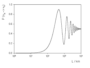
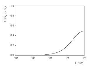
Figure 3: Atmospheric neutrino oscillation probability (10), including quantum decoherence parameters which are independent of the neutrino energy, plotted as a function of path length $L$ (measured in km), for fixed neutrino energy $E$ equal to 1 GeV (top) and 200 GeV (bottom).

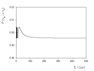
Figure 4: Atmospheric neutrino oscillation probability (10), including quantum decoherence parameters which are independent of the neutrino energy, plotted as a function of neutrino energy $E$ (measured in GeV), for fixed path length equal to 10000 km.

The graphs in figures 3 and 4 should be compared with those in figures 1 and 2 respectively. The effect of the quantum decoherence can be clearly seen. At low energy ($E=1$ GeV), the standard oscillations are damped by quantum decoherence until the oscillation probability converges to one half (corresponding to complete decoherence) at a path length of about $10^{4}$ km. However, at high energy ($E=200$ GeV), the difference caused by quantum decoherence is highly marked (note the different vertical scales in the graphs in figures 1 and 3), with a large enhancement of the oscillation probability. This enhancement of the oscillation probability at large path lengths can also be seen by comparing figures 2 and 4. For standard oscillations, the probability tends to zero for fixed path length and increasing energy, but this is not the case when quantum decoherence is included, the damping factor in the oscillation probability (10) ensuring that the oscillation probability tends to a limiting value for large energy at fixed path-length.

For larger values of the decoherence parameters, these effects become even more marked, and, for sufficiently large decoherence parameters, the oscillations may be damped away completely, even at low energy. This is in effect what has happened at high energy in figure 3. As would be expected, as we decrease the magnitudes of the decoherence parameters, the decoherence effects become less significant and the probabilities become indistinguishable from those for standard neutrino oscillations. However, even for very small quantum decoherence parameters, there may be significant effects at high energy. For example, in figure 5, we plot the oscillation probability for fixed path length and varying energy for the case in which the quantum decoherence parameters are proportional to the neutrino energy squared.

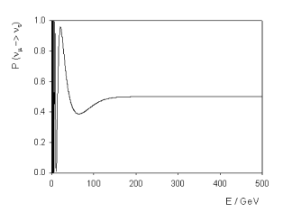
Figure 5: Atmospheric neutrino oscillation probability including quantum decoherence parameters which are proportional to the neutrino energy squared, plotted as a function of neutrino energy $E$ (measured in GeV), for fixed path length equal to 10000 km.

In this situation, the bounds we find in section 5 are very strong, and the oscillation probability for low energy neutrinos is indistinguishable from that for standard neutrino oscillations. However, as can be seen in figure 5, there is a significant change in the neutrino oscillation probability at high energy.

The values of the quantum decoherence parameters used in producing figure 5 are sufficiently small that they have not been ruled out by current atmospheric neutrino oscillation data [10]. It is clear from figure 5 that high energy neutrinos are necessary in order to probe such quantum decoherence effects, and it is the main result of this paper that neutrino telescopes such as ANTARES are indeed able to perform this, in contrast to comparatively low-energy experiments. We would expect the bounds we discuss in section 5, attainable with atmospheric neutrino data, to be further tightened with neutrinos of astrophysical rather than atmospheric origin [41].

4 Specific Models of Quantum Decoherence

In this section we now discuss in detail specific models of quantum decoherence. The most general time evolution equation including quantum decoherence effects (5) involves six parameters additional to those for the standard neutrino oscillations. It is not possible to derive analytically in a simple closed form a general oscillation probability involving all six extra parameters, and either a numerical approach or an approximation scheme would be necessary [5, 6]. Furthermore, it is unlikely that, at least to begin with, experimental data will be able to produce meaningful bounds/fits for all six additional parameters. In view of the above, we shall consider models in which only two or fewer of the quantum decoherence parameters $\alpha$, $\beta$, $\delta$, $a$, $b$, or $d$ are non-zero, but we study different combinations of these parameters in order to incorporate different possible effects.

Various models have been considered in the literature to date (see, for example, [5, 6, 7, 8, 9]), although the only work of which we are aware involving analysis of experimental data is [10, 11]. The models which have received most attention to date are those with $a$, $\alpha$ and $b$ non-zero but $d$, $\beta$ and $\delta$ zero [5, 7, 8] and those where $\alpha$, $\beta$ and $\delta$ are non-zero but $a$, $b$ and $d$ vanish [5, 6, 8, 9]. Benatti and Floreanini [5] consider a quite general model (all parameters non-zero) initially, but later concentrate on the case when $d=\beta=0$ and also $\delta=0$, although they impose the condition of complete positivity. They also consider all parameters non-zero using a second order approximation. Our models below are all special cases of the models considered by Benatti and Floreanini. Liu and collaborators [6] set $a=b=d=0$, although in this case the oscillation probability can only be computed numerically. Here we either set both $a$ and $\alpha$ to be zero, or both are non-zero, so our probabilities do not tally with theirs. Chang et al [8] consider the same model as [6], but set $\beta=0$ in order to obtain an analytic probability. Again, our models do not fit into their picture. They also consider the leading order corrections to the standard oscillation probability for $a$, $b$, and $\alpha$ non-zero and $d$, $\beta$, and $\delta$ vanishing. Ma and Hu [7] work with the second of Chang et al’s models, this time with exact analytic results for the oscillation probability. Models 1 - 4 below consider various combinations of parameters within this model. Finally, Klapdor-Kleingrothaus and collaborators [9] consider a model in which only $\alpha$ and $\delta$ are non-zero.

We first consider a class of models in which we set $d$ and $\beta$ equal to zero, so that both the terms $M_{13}(E,L)$ and $M_{31}(E,L)$ in equation (7) vanish. The forms of the quantities $M_{11}(E,L)$ and $M_{33}(E,L)$ in equation (7) are derived by solving the differential equations (6) describing the time evolution of the components of the density matrix, using suitable initial conditions. The answer (with $c=\hbar=1$) is:

$$M_{11} = \left\{\begin{array}[]{ll}e^{-\Gamma_{{\rm{sum}}}}\cos\Gamma_{1}&{\mbox{if $a=\alpha$;}}\\ e^{-\Gamma_{{\rm{sum}}}}\left(\cos\Gamma_{2}+\frac{\Gamma_{{\rm{diff}}}}{\Gamma_{2}}\sin\Gamma_{2}\right)&{\mbox{if $b=0$;}}\end{array}\right.$$ (13)

$$M_{33} = e^{-2\delta L};$$ (14)

with

$$\Gamma_{{\rm{sum}}} = \left(\alpha+a\right)L;$$

$$\Gamma_{{\rm{diff}}} = \left(\alpha-a\right)L;$$

$$\Gamma_{1} = 2\left[\left(\frac{\Delta m^{2}L}{4E}\right)^{2}-b^{2}L^{2}\right]^{\frac{1}{2}};$$

$$\Gamma_{2} = 2\left[\left(\frac{\Delta m^{2}L}{4E}\right)^{2}-\frac{1}{4}\left(\alpha-a\right)^{2}L^{2}\right]^{\frac{1}{2}}.$$ (15)

Setting the quantum decoherence parameters in equations (14-15) equal to zero, we recover the standard oscillation probability. The other limit of interest is if we set the standard oscillation parameter $\Delta m^{2}=0$ (but keeping the usual mixing angle $\theta$ non-zero). In this case atmospheric neutrino oscillations would be due to quantum decoherence effects only. Given the widespread acceptance of the standard oscillation picture, such a scenario may seem highly unlikely, but the only existing analysis of experimental data [10, 11] found that, while oscillations due to quantum decoherence only are unfavoured by the experimental data, the evidence is not overwhelming. However, in this paper we shall mostly be concerned with quantum decoherence effects as modifications of the standard picture. If we do set $\Delta m^{2}=0$ in equation (15), it is clear that we can obtain a sensible oscillation probability only if $\Gamma_{1}$ and $\Gamma_{2}$ are real, which means that $a=\alpha$ and $b=0$. If, however, $\Gamma_{1}$ and $\Gamma_{2}$ are imaginary when $\Delta m^{2}=0$, it is possible to write the oscillation probability in terms of exponential (damping) terms only, without any oscillations. Given the success of the phenomenology of neutrino oscillations, we do not consider this possibility further.

The parameter $\delta$ corresponds to energy non-conserving effects in the atmospheric neutrino system. However, since the terms in the probability (7) which contain $\delta$ are multiplied by $\cos^{2}(2\theta)$, and the current experimental best-fit value for $\cos^{2}(2\theta)$ is zero [11], this energy non-conserving parameter has a negligible effect on the oscillation probability, and so we will not consider it further in this section. However, see section 6 for bounds on this parameter from other experiments. The models of this first type we shall consider are therefore:

1. The simplest possible model is when $b=\delta=0$ and $a=\alpha\neq 0$. It is this model which has been studied for Super-Kamiokande and K2K data [10, 11], and the time evolution of the density matrix satisfies the conditions of complete positivity and energy conservation within the atmospheric neutrino system. Furthermore, only in this model does the time-evolution of the density matrix (2) have the Lindblad form (3).

2. We set $b=\delta=0$, with $a$ and $\alpha$ non-zero but not equal. This is the simplest possible generalization of the previous model; and energy is conserved in this case (as it is in the next two models as well). This model is probably the most likely generalization to be of experimental significance, since the consensus in the literature is that $b$ will be significantly smaller than either $a$ or $\alpha$. However, this model violates the condition of complete positivity [5]. In this and the following two models, oscillations cannot be accounted for solely by quantum decoherence, and we must include a non-zero $\Delta m^{2}$ in the probability.

3. In our third model we consider only a non-zero $b$ in (15), setting all other quantum decoherence parameters (including $a$ and $\alpha$) to vanish. The form of the probability (7) is such that the sign of $b$ cannot be measured, so we assume from henceforth that $b$ is positive (equivalently, we are considering only $|b|$). In the literature, the assumption is frequently made that $b$ will be much smaller than either $a$ or $\alpha$, which would rule this model out. However, we include it here so that we can look specifically at the effect of $b$ on the system. Like the previous model, this one also violates complete positivity [5].

4. Our next model is, in effect, a combination of the previous two. We set $a=\alpha$ and $b$ to be non-zero, but have $\delta$ and all other quantum decoherence parameters vanishing. Even this more general model does not satisfy complete positivity [5] as we have set $\delta=0$. In studying this model in the next section, we find no additional information on the parameter space of $\alpha$, $a$ and $b$ than we did by studying models 2 and 3, which implies that it is sufficient to consider varying the quantum decoherence parameters separately, at least as far as finding upper bounds on sensitivity regions is concerned.

Our second class of models violate energy conservation within the atmospheric neutrino system. We set $a=b=\alpha=\delta=0$ and consider instead non-zero $d$ and $\beta$. The oscillation probability will have the general form (7). Although, because the mixing angle $\theta$ for atmospheric neutrino oscillations is such that $\cos^{2}(2\theta)$ is very close to zero, we are unable to measure $M_{33}$, $M_{31}$ or $M_{13}$ directly, there are, in the two models below, also modifications of $M_{11}$ which we can probe, and so measure these other quantities indirectly. This is in contrast to the situation in which the parameter $\delta$ is non-zero, as this shows up only in $M_{33}$ if $d=\beta=0$. The models we consider are therefore:

1. Firstly, we set all parameters equal to zero except $\beta$. The oscillation probability (7) in this case is

   $$P[\nu_{\mu}\rightarrow\nu_{\tau}] = \frac{1}{2}\left\{\cos^{2}2\theta\left[1-\frac{\omega^{2}}{\Omega_{\beta}^{2}}+\frac{\beta^{2}}{\Omega_{\beta}^{2}}\cos(2\Omega_{\beta}L)\right]\right.$$ (16)

   $$\left.+\sin^{2}2\theta\left[1+\frac{\beta^{2}}{\Omega_{\beta}^{2}}-\frac{\omega^{2}}{\Omega_{\beta}^{2}}\cos(2\Omega_{\beta}L)\right]\right\}$$

   where $\Omega_{\beta}=\sqrt{\omega^{2}-\beta^{2}}$ and $\omega=\frac{\Delta m^{2}}{4E}$. In both this model and the next, it is not possible for oscillations to be due to decoherence only, as the argument of the $\cos$ term becomes imaginary if we set $\Delta m^{2}=0$. The probability (16) contains only $\beta^{2}$ terms and so we consider only $\beta>0$ (or, equivalently, $|\beta|$).

2. In this model, we set all the quantum decoherence parameters to zero except $d$. The probability of oscillation (7) in this case has the form:

   $$P[\nu_{\mu}\rightarrow\nu_{\tau}] = \frac{1}{2}\left\{\cos^{2}2\theta\left[1-\frac{\omega^{2}}{\Omega_{d}^{2}}+\frac{d^{2}}{\Omega_{d}^{2}}\cos(2\Omega_{d}L)\right]\right.$$ (17)

   $$\left.+\sin^{2}2\theta\left[1+\frac{d^{2}}{\Omega_{d}^{2}}\cos(2\Omega_{d}L)-\frac{\omega^{2}}{\Omega_{d}^{2}}\cos(2\Omega_{d}L)\right]\right.$$

   $$\left.+\sin 4\theta\left[\frac{d}{\Omega_{d}}\sin(2\Omega_{d}L)\right]\right\}$$

   where $\Omega_{d}=\sqrt{\omega^{2}-d^{2}}$. This is the only model in which the quantities $M_{13}(E,L)$ and $M_{31}(E,L)$ are non-zero. Although both $d$ and $d^{2}$ appear in the probability (17), in fact only $d^{2}$ can be measured with atmospheric neutrinos because $\sin 4\theta\sim 0$. Therefore we consider only $d>0$ (or $|d|$).

We are now in a position to examine ANTARES sensitivity to these quantum decoherence effects.

5 ANTARES sensitivity to quantum decoherence in atmospheric neutrino oscillations

ANTARES is sensitive to high energy atmospheric neutrinos, with energy above 10 GeV [13]. Although in some sense these are a background to the neutrinos of astrophysical origin which are the main study of a neutrino telescope, nevertheless the detection of very high energy atmospheric neutrinos which have very long path lengths (of the order of the radius of the Earth) is complementary to other long baseline neutrino experiments such as MINOS [24], OPERA [25], K2K [42], KamLAND [43] and CHOOZ [44]. Our analysis of the sensitivity of ANTARES to quantum decoherence effects in atmospheric neutrinos is based on a modification of the analysis of standard atmospheric neutrino oscillations with ANTARES [13, 45]. We would anticipate that other high energy neutrino telescopes such as AMANDA [20] and ICECUBE [21] would also be able to probe these effects.

5.1 Simulations and analysis

Our simulations are based on previous ANTARES simulations of the sensitivity to standard neutrino oscillations [45]. Further details of the ANTARES detector, detector simulation and event signals can be found in [45]. Here we summarize the main features of the simulations which are pertinent to our discussion. Atmospheric neutrinos events were generated using Monte-Carlo production. A spectrum proportional to $E^{-2}$ for the neutrinos was assumed, for energies in the range 10 GeV $<E<$ 100 TeV. The zenith angle distribution is assumed to be isotropic. Twenty-five years of data were simulated, so that errors from the MC statistics could safely be ignored. Event weights were used to adapt the MC flux to a real atmospheric neutrino flux. We used the Bartol theoretical flux [46], although the results will not be significantly changed by using different theoretical fluxes. There may be a more significant change in our results if the spectral index is modified.

Our simulations are based on three years’ data taking with ANTARES. This corresponds to roughly 10000 atmospheric neutrino events. All errors are purely statistical, with simple Gaussian errors assumed. By varying the form of the oscillation probability to include quantum decoherence effects, spectra in either $E$, $E/L$ or $L$ are produced. Some examples of these are discussed in the next subsection. Since ANTARES is particularly sensitive to the zenith angle $\vartheta$ and thereby the path length $L$, the spectra in $E/\cos\vartheta$ are used in the sensitivity analysis.

To produce sensitivity regions, we used a $\chi^{2}$ technique, comparing the $\chi^{2}$ for oscillations with decoherence (or decoherence alone) with that for the no-oscillation hypothesis. The total normalization is left as a free parameter in the sensitivity analysis, so that our results in section 5.3 are not affected by the normalization of the atmospheric neutrino flux. The sensitivity regions at both 90 and 99% confidence level are produced.

Even though our analysis is independent of the normalization of the atmospheric neutrino flux, in order to produce spectra based on numbers of events, as in the following subsection, some normalization of the total flux is necessary. For standard oscillations without quantum decoherence, bins with high $E/\cos\vartheta$ can be used to normalize the flux as standard oscillations are negligible at sufficiently high $E/L$ (as can be seen in figure 1). This method can also be applied for quantum decoherence models in which the decoherence parameters are inversely proportional to the neutrino energy, so that decoherence also becomes negligible at high energy. However, when the decoherence parameters are proportional to the neutrino energy squared, decoherence is significant at high energies but negligible at low $E/L$. Therefore, in this latter case, we may use the low $E/\cos\vartheta$ bins to normalize the flux.

We have studied six different models of quantum decoherence, as outlined in the previous section, and for each model there are three different ways in which the quantum decoherence parameters may depend on the neutrino energy. We shall not discuss the details of all eighteen of our simulations, but instead summarize our results and discuss a few models in more detail to illustrate the essential features. In our simulations, for practical reasons, we had at most three varying parameters, one of which was always the mixing angle $\theta$ which facilitated comparisons with previous work [10, 11, 45]. In models with only one non-zero decoherence parameter (namely models 1, 3, 5 and 6 above) we also varied $\Delta m^{2}$, to check that our sensitivity regions included the current best-fit values [10, 11]. In models with two non-zero decoherence parameters (models 2 and 4), we fixed $\Delta m^{2}=2.6\times 10^{-3}$ eV². The simulations then give us a three-dimensional region of sensitivity at 90 and 99 percent confidence level, and we plotted the boundaries of the projections of the surface bounding this volume onto the co-ordinate planes, where necessary also plotting the surface itself.

5.2 Spectra

As well as data based on total numbers of events, the spectra of these events in (typically) $E/L$ is also important in neutrino oscillation physics. For atmospheric neutrinos, Super-Kamiokande [12] has reported an oscillatory signature in the $E/L$ spectrum of events, and similar spectral analyses have been performed for KAMLAND [23] and K2K [47]. As well as being used in our analysis of sensitivity regions, the spectra themselves are important for searching for possible decoherence effects and also for bounding the size of such effects. The overall normalization of the flux, required to produce these spectra, can be found using either the high or low $E/\cos\vartheta$ bins, depending on the situation, as described in the previous subsection.

Figures 6, 7 show typical spectra of events as a function of $E/\cos\vartheta$ (corresponding to $E/L$), where $E$ is the reconstructed energy and $\vartheta$ the zenith angle, not to be confused with the mixing angle $\theta$. In each case, the solid line is the MC simulation with standard oscillations and no decoherence, using the values of the oscillation parameters in (9), while the dotted and dashed lines are the MC simulation with standard oscillations and decoherence together.

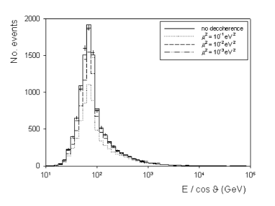
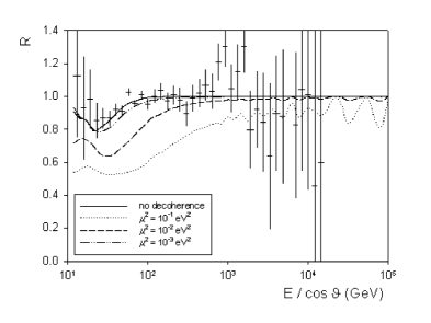
Figure 6: Spectrum of events as a function of $E/\cos\vartheta$ (top) and ratio of the number of events compared to no oscillations (bottom). In each graph, the solid line represents MC simulation of standard oscillations without decoherence, and the dotted lines represent MC simulation of standard oscillations plus decoherence. The data points correspond to a three-year measurement, assuming standard oscillations only without decoherence. The decoherence parameters are inversely proportional to the neutrino energy.

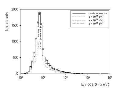
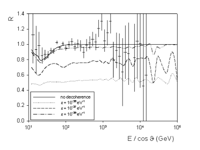
Figure 7: Spectra of events as in figure 6 but for the case when the decoherence parameters are proportional to the neutrino energy squared.

The spectra in figure 6 are for the model in which the quantum decoherence parameters are inversely proportional to the neutrino energy, while in figure 7 we consider quantum decoherence parameters which are proportional to the neutrino energy squared. In both figures 6, 7, we have also plotted the ratio of the number of events compared with no oscillations. It can be seen that in both cases quantum decoherence results in a significant reduction in the number of events. However, there is also a difference in the shape of the spectra. In both models, when the decoherence parameters are comparatively large, the spectrum in the ratio of the number of events (lower plots) is much flatter in the region below about 150 GeV, compared with standard oscillations (when there is a ‘dip’ in the ratio of the number of events). For the case in which the decoherence parameters are inversely proportional to the neutrino energy, the ratio of the number of events rises to one at very high energies, but more slowly than the case of oscillations only. However, it should be stressed that the values of the parameter $\mu^{2}$ for which this is most noticeable in figure 6 are larger than the current best upper bound from SK and K2K data [11]. When the decoherence parameters are proportional to the neutrino energy squared (figure 7), the spectrum of the ratio of the number of events is extremely flat.

We can also consider the situation in which there are no standard oscillations, in other words, the squared mass difference $\Delta m^{2}$ is zero. In this case, neutrino oscillations would be described entirely by decoherence. In this case the ratios of the numbers of events compared with the no-oscillation hypothesis are shown in figure 8, for decoherence parameters inversely proportional to the neutrino energy (upper plot) and proportional to the neutrino energy squared (lower plot).

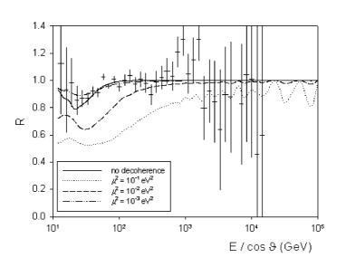
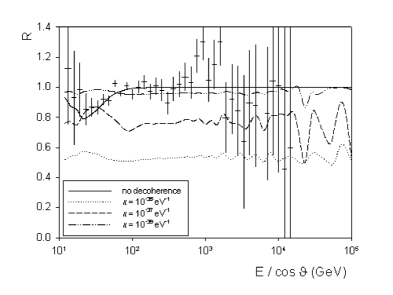
Figure 8: Ratios of the number of events compared to no oscillations, as functions of $E/\cos\vartheta$. The solid line is for standard oscillations only without decoherence, for comparison. The remaining curves are for no standard oscillations, and quantum decoherence only. The upper plot is for quantum decoherence parameters inversely proportional to the neutrino energy, and the lower plot for the case when the quantum decoherence parameters are proportional to the neutrino energy squared.

We have plotted in figure 8 the ratio for the standard oscillations only case for comparison (the solid line), but the other curves are for pure decoherence without standard oscillations. The difference in the spectra at $E/\cos\vartheta$ below about 150 GeV is clear for the case when the decoherence parameters are proportional to the neutrino energy squared, with the decoherence-only model generally producing a peak in the spectrum where standard oscillations without decoherence has a dip. When the decoherence parameters are inversely proportional to the neutrino energy, the spectra look more like those for standard oscillations plus decoherence (figure 6), except for small values of $\mu^{2}$, when the spectrum is flatter than for standard oscillations only.

It should be emphasised that the values of the quantum decoherence parameter $\kappa$ used to generate the spectra in figures 7 and 8 are many orders of magnitude smaller than the current experimental upper bound of $10^{-19}$ eV^-1 [10]. As the decoherence parameter $\kappa$ increases, the number of events decreases and so it is clear from figures 7 and 8 that ANTARES will be able to rule out even very small values of $\kappa$. This can be understood from the oscillation probabilities as shown in the figures in section 3. For high energy neutrinos, the standard oscillation probability is negligible and so the number of events depends only on the atmospheric neutrino flux. However, with quantum decoherence, the oscillation probability becomes close to one-half for atmospheric neutrinos and so a large fraction of the incoming muon neutrinos will oscillate, resulting in a significant decrease in the number of events seen. For low energy neutrinos, as observed by current atmospheric neutrino experiments, in the model we have concentrated on in this subsection, the effects of quantum decoherence are negligible with these values of the quantum decoherence parameters because the effects are proportional to the neutrino energy squared.

This is the main result of our paper: ANTARES measures high-energy neutrinos and so will be able to put stringent bounds on quantum decoherence effects which are proportional to the neutrino energy squared.

5.3 Sensitivity regions

We now turn to a discussion of the ANTARES sensitivity regions from our simulations. We discuss the simplest model in some detail as it reveals most of the salient features. The remaining models are summarized briefly. We are particularly interested in the upper bounds on the sensitivity regions. We focus mainly on the case where the quantum decoherence parameters are proportional to the neutrino energy squared, as here we will have the most significant improvement on current experimental bounds.

5.3.1 Model 1

This is the model in which $\alpha=a$ and has been studied for Super-Kamiokande and K2K data [10, 11]. They found the best fit to the data when the quantum decoherence parameter is inversely proportional to the neutrino energy [10]. A detailed analysis [11] of this case then found that the favoured situation was standard oscillations without decoherence, but that the data could not entirely rule out oscillations due to quantum decoherence only. We show our results for this model with the parameters $\alpha=a$ inversely proportional to the neutrino energy in detail for comparison purposes, but our main results are concerned with the case in which the parameters are proportional to the neutrino energy squared, as it is in this latter case that we can significantly improve current bounds.

Firstly, consider the case in which $\Delta m^{2}=0$, so that there are no standard oscillations and only quantum decoherence. Figure 9 shows the sensitivity curves in this case, for $\alpha=a$ inversely proportional to the neutrino energy, and figure 10 for $\alpha=a$ proportional to the neutrino energy squared.

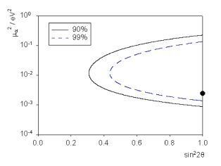
Figure 9: Sensitivity contours at 90 and 99 percent confidence level for quantum decoherence effects only (no standard oscillations), with parameter $\mu_{\alpha}^{2}$. The circle denotes the value $\mu_{\alpha}^{2}=2.44\times 10^{-3}$ eV², which is the best fit to combined Super-Kamiokande and K2K data [11].

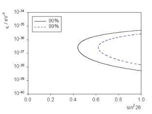
Figure 10: Sensitivity contours at 90 and 99 percent confidence level for quantum decoherence effects only (no standard oscillations), with parameter $\kappa_{\alpha}$.

It is somewhat surprising that current experimental data [11] only slightly disfavours this model, in comparison to the standard oscillation picture. The best fit value for combined Super-Kamiokande and K2K data is $\mu_{\alpha}^{2}=2.44\times 10^{-3}$ eV² with $\sin^{2}(2\theta)=1.00$ [11], which lies within our region of sensitivity, and is shown by a solid circle in figure 9. However, the K2K data taken alone has a best fit of $\mu_{\alpha}^{2}=2.46\times 10^{-3}$ eV², with $\sin^{2}(2\theta)=0.86$ [11]. It is clear from figure 9 that the smallest values of $\mu_{\alpha}^{2}$ can be probed when $\sin^{2}(2\theta)$ is closest to one, which is the region of parameter space in which we are most interested. It is also interesting to note the similarity in the value of $\mu_{\alpha}^{2}$ to that of $\Delta m^{2}$ for standard oscillations.

For the case in which $\alpha=a$ are proportional to the neutrino energy squared, it is important to note that the range of values of the parameter $\kappa_{\alpha}$ shown in figure 10 is many orders of magnitude lower than the current upper bound of $10^{-19}$ eV^-1 [10]. Therefore ANTARES will be able to probe regions of parameter space currently inaccessible to lower-energy experiments, and improve significantly on existing experimental bounds.

We also studied pure decoherence for the case in which $\alpha=a$ do not depend on the neutrino energy. The sensitivity curves in this case have a very similar shape to those in figures 9 and 10, with sensitivity to values of the parameter $\gamma_{\alpha}$ in the region $10^{-13}$ – $10^{-14}$ eV, which is a similar range to the current upper bound from SK data of $10^{-14}$ eV [10].

We also found sensitivity curves for the more general case when both $\Delta m^{2}$ and $\mu_{\alpha}^{2}$, $\kappa_{\alpha}$ or $\gamma_{\alpha}$ (as applicable) are non-zero. The results we obtained are shown in figures 11 and 12 for the $\mu_{\alpha}^{2}$ and $\kappa_{\alpha}$ cases, respectively. We do not show the graphs for the $\gamma_{\alpha}$ case because they are qualitatively very similar to the $\mu_{\alpha}^{2}$ case. In figures 11 and 12, we have plotted projections of a three-dimensional volume onto each of the co-ordinate planes, and the contours represent the boundaries of the projected regions.

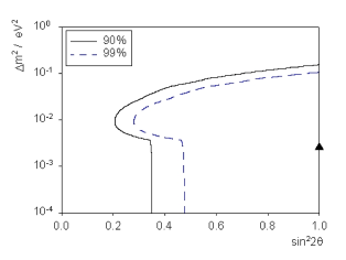
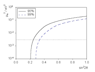
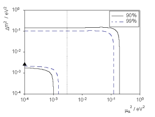
Figure 11: Sensitivity contours at 90 and 99 percent confidence level, when both oscillation and quantum decoherence parameters ($\mu_{\alpha}^{2}$) are non-zero. The dotted line denotes the bound $\mu_{\alpha}^{2}<3\times 10^{-3}$ eV² from Super-Kamiokande and K2K data [11], and the triangle the best fit value $\Delta m^{2}=2.6\times 10^{-3}$ eV², $\sin^{2}(2\theta)=1$ [11].

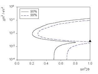
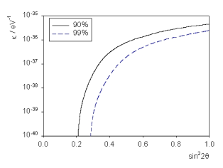
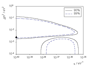
Figure 12: Sensitivity contours at 90 and 99 percent confidence level, when both oscillation and quantum decoherence parameters ($\kappa_{\alpha}$) are non-zero. The triangle denotes the best fit value $\Delta m^{2}=2.6\times 10^{-3}$ eV², $\sin^{2}(2\theta)=1$ [11].

The sensitivity contours should be compared with the combined Super-Kamiokande and K2K results [11]. In each figure, the best fit values of $\Delta m^{2}=2.6\times 10^{-3}$ eV² and $\sin^{2}(2\theta)=1$ [11] are denoted by a triangle, while the upper bound $\mu_{\alpha}^{2}<3\times 10^{-3}$ eV² [11] is marked by a dotted line in figure 11. Our regions have a very similar shape to those constructed from data in [11].

For the situation in which the quantum decoherence parameters are inversely proportional to the neutrino energy (figure 11), it should be noted that the upper bound on the sensitivity region at $\sin^{2}(2\theta)=1$ is considerably higher than the upper bound from data [11]. This is to be expected since ANTARES measures only high energy atmospheric neutrinos (energy greater than 10 GeV compared with a few GeV for Super-Kamiokande [48] and K2K [42]) and so is likely to be comparatively insensitive to effects inversely proportional to the neutrino energy. However, when the decoherence parameters are proportional to the neutrino energy squared (figure 12), the upper bound on the sensitivity region, $\kappa_{\alpha}<10^{-35}$ eV ^-1, is many orders of magnitude smaller than the corresponding bound from Super-Kamiokande data of $10^{-19}$ eV^-1 [10]. In the final case, when the quantum decoherence parameters are independent of the neutrino energy, we find an upper bound on the sensitivity region of $\gamma_{\alpha}<10^{-14}$ eV, which is of a similar order of magnitude to the bound from Super-Kamiokande data of $10^{-14}$ eV [10].

5.4 Models 2, 3 and 4

These models involve combinations of the quantum decoherence parameters $a$, $\alpha$ and $b$. The upper bounds of the sensitivity regions that we find for a particular parameter are essentially independent of the particular combination of other parameters chosen to be non-zero, and whether or not we fix $\Delta m^{2}$. The parameters $a$ and $\alpha$ have the same sensitivity regions when they are not necessarily equal, and whenever the parameter $b$ is included, it has a upper bound corresponding to the value at which the factors $\Gamma_{1}$ and $\Gamma_{2}$ (15) (as applicable) become imaginary.

As an illustration of our results in these models, we plot in figure 13 the sensitivity curves for the model in which $a=\alpha\neq 0$, $b\neq 0$, $\Delta m^{2}$ is fixed at its best fit value (9) [11], and with the quantum decoherence parameters proportional to the neutrino energy squared, as it is in this case that we have the most stringent bounds on quantum decoherence effects.

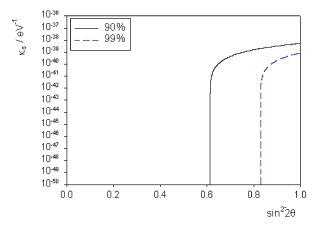
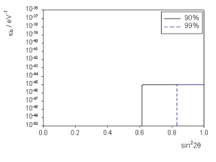
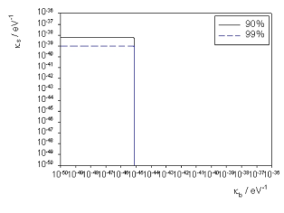
Figure 13: Sensitivity contours at 90 and 99 percent confidence levels, with two non-zero decoherence parameters which are proportional to the neutrino energy squared and given in terms of the constants $\kappa_{s}=\kappa_{\alpha}=\kappa_{a}$ and $\kappa_{b}$.

We find upper bounds on the sensitivity regions of $\kappa_{s}=\kappa_{a}=\kappa_{\alpha}<10^{-38}$ eV^-1 and $\kappa_{b}<10^{-45}$ eV^-1. As with model 1, these bounds are very strong, and it is interesting to note that our bound on $\kappa_{a}=\kappa_{\alpha}$ is a couple of orders of magnitude smaller in this model than it was in model 1.

If the quantum decoherence parameters are independent of the neutrino energy, we find upper bounds to our sensitivity regions of $\gamma_{a}=\gamma_{\alpha}<10^{-13}$ eV and $\gamma_{b}<10^{-16}$ eV, this latter value again being due to the cut-off in $b$. For the third possibility, when the quantum decoherence parameters are inversely proportional to the neutrino energy, our upper bounds are somewhat weaker, at $\mu^{2}_{\alpha}=\mu^{2}_{a}<10^{0}$ eV², and $\mu^{2}_{b}<10^{-2}$ eV².

5.4.1 Model 5

To illustrate the typical sorts of plots we get for the sensitivity curves, we show in figure 14 the sensitivity contours for this model in the case in which the quantum decoherence parameter proportional to the neutrino energy squared and given by $\kappa_{\beta}$.

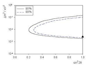
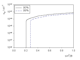
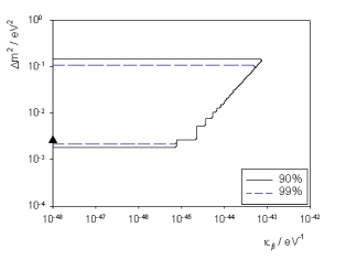
Figure 14: Sensitivity contours at 90 and 99 percent confidence levels, for model 5 with both standard oscillations and non-zero decoherence parameter $\kappa_{\beta}$. The triangle shows the experimental point of best fit for $\Delta m^{2}$ [11].

There is again a cut-off in the parameter $\kappa_{\beta}$ due to the probability (16) becoming imaginary, and this can be clearly seen in the plots. Our upper bound on $\kappa_{\beta}$ is $10^{-43}$ eV^-1 in this case. The plots shown in figure 14 are typical of those found in many of our models for the different quantum decoherence parameters, when we also vary $\Delta m^{2}$.

When the quantum decoherence parameters are independent of the neutrino energy, the sensitivity regions are qualitatively the same as those in figure 14, and we find an upper bound $\gamma_{\beta}<10^{-15}$ eV. However, when the quantum decoherence parameters are inversely proportional to the neutrino energy, the situation is rather more complicated, and we need to examine the surface in three-dimensional parameter space which bounds the sensitivity region. This is shown in figure 15 for 90% confidence level.

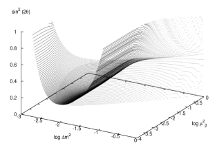
Figure 15: The boundary of the volume in parameter space at 90% confidence level, for model 5 with both standard oscillations and a non-zero decoherence parameter $\mu_{\beta}^{2}$. The sensitivity region lies above this surface.

The region of interest lies above the surface in figure 15, including the value $\sin^{2}(2\theta)=1$. For small values of $\mu_{\beta}^{2}$, it is clear that this region is similar in shape to the previous figure 14. However, for larger values of $\mu^{2}_{\beta}$, the surface opens out and all values of $\Delta m^{2}$ and $\sin^{2}(2\theta)$ are included. Because of this, we are unable to place an upper bound on $\mu^{2}_{\beta}$ in this case. This is not entirely unexpected because ANTARES measures high energy neutrinos, so that its ability to place bounds on effects inversely proportional to neutrino energy is limited.

5.4.2 Model 6

This model is somewhat different to any considered before as the parameter $d$ is non-zero and so the oscillation probability (17) has contributions from the $\sin 4\theta$ term. However, the sensitivity regions are broadly similar to those in the previous model. We find the following upper bounds on the sensitivity regions:

$$\gamma_{d}<10^{-15}\,\,{\mbox{eV}};\qquad\qquad\mu^{2}_{d}<10^{-1}\,\,{\mbox{eV${}^{2}$}};\qquad\qquad\kappa_{d}<10^{-43}\,\,{\mbox{eV${}^{-1}$}}.$$

6 Comparing experimental bounds on decoherence parameters

In this section we compare our upper bounds on quantum decoherence parameters, from simulations, with existing experimental data. Firstly, for ease of comparison, we restate, in table 1, the upper bounds of the constants of proportionality $\gamma$, $\mu^{2}$ and $\kappa$ for each of the quantum decoherence parameters, changing the units to GeV for ease of comparison with other references.

model	$a$	$|b|$	$|d|$	$\alpha$	$|\beta|$
$\gamma({\mbox{GeV}})$	$9\times 10^{-23}$	$7\times 10^{-25}$	$7\times 10^{-25}$	$9\times 10^{-23}$	$7\times 10^{-25}$
$\mu^{2}({\mbox{GeV${}^{2}$}})$	$2\times 10^{-19}$	$6\times 10^{-19}$	$6\times 10^{-19}$	$2\times 10^{-19}$	-
$\kappa({\mbox{GeV${}^{-1}$}})$	$4\times 10^{-26}$	$7\times 10^{-35}$	$7\times 10^{-35}$	$4\times 10^{-26}$	$7\times 10^{-35}$

Table 1: Table showing the upper bounds of the constants of proportionality in the quantum decoherence parameters from simulations for different dependences on the neutrino energy.

Upper bounds have been placed on the decoherence parameters [10, 11] by examining data from the Super-Kamiokande and K2K experiments. We note than the bounds for the $\gamma$ model ($\gamma_{\alpha}<3.5\times 10^{-23}$ GeV) are entirely consistent with those found in our simulations, the bounds for the $\mu^{2}$ model ($\mu_{\alpha}^{2}<2.44\times 10^{-21}$ GeV²) are slightly better than the ANTARES bounds whereas the bounds found for the $\kappa$ model ($\kappa_{\alpha}<9\times 10^{-10}$ GeV^-1) are much worse than our bounds. The ANTARES bounds are found with high energy neutrinos whereas Super-Kamiokande detects lower energy neutrinos and so we see that experiments which are more sensitive to lower energy neutrinos are better probes of the $\mu^{2}$ model whilst those with sensitivity to higher energy neutrinos are much better at placing bounds on the quantum gravity parameters using the $\kappa$ model. For each quantum decoherence parameter, our upper bounds on the constant $\kappa$ are particularly strong, and, given that $\kappa$ contains one inverse power of the Planck mass ($10^{19}$ GeV), are close to ruling out such effects.

The neutrino system is not the only quantum system which may be affected by interactions with space-time foam. Experiments such as CPLEAR [49] have examined this problem with neutral kaons, and found the upper bounds on the quantum decoherence parameters to be [50]

$$a<4\times 10^{-17}\,\,{\mbox{GeV}},\qquad|b|<2.3\times 10^{-19}\,\,{\mbox{GeV}},\qquad\alpha<3.7\times 10^{-21}\,\,{\mbox{GeV}}.$$

A second analysis of this experiment took place in reference [19] with six quantum decoherence parameters. The authors of reference [19] were able to put bounds all the parameters and they found upper bounds on the quantum decoherence parameters to be of order $10^{-17}-10^{-18}$ GeV. It is difficult to directly compare our results with these bounds due to the dependence on the neutrino energy in some of our models. However, when the quantum decoherence parameters are constants, our upper bounds on $\gamma$ from table 1 lead to upper bounds on the decoherence parameters themselves of

$$a=\alpha<5\times 10^{-23}\,\,{\mbox{GeV}},\qquad|b|=|d|=|\beta|<3\times 10^{-25}\,\,{\mbox{GeV}},$$

and so, it seems that the ANTARES experiment will be able to improve the upper bounds of these parameters with respect to the CPLEAR experiment.

Quantum decoherence has also been explored using neutron interferometry experiments, as suggested in [4]. In reference [51], upper bounds on the parameters $a$ and $\alpha$ were found using data from such an experiment:

$$a\leq 1\times 10^{-22}\,\,{\mbox{GeV}},\qquad\alpha\leq 7.4\times 10^{-22}\,\,{\mbox{GeV}}.$$

Once again, our upper bounds are tighter than these values. It is interesting to note that in both the kaon and neutron experiments, the quantum decoherence parameter $a\neq\alpha$ whereas in the neutrino system, we find $a=\alpha$. This variation arises from the different mixing in these systems. The other difference between the meson and neutrino experiments is the possibility of different decoherence effects in the anti-neutrino sector as compared with the neutrino sector [35, 36], although we have not considered this possibility further in this paper.

7 Other effects on atmospheric neutrino oscillations

Quantum decoherence is not the only process which may modify the standard oscillation probability (8) for atmospheric neutrinos. In this section we briefly discuss some of the other possible phenomena, indicating how they change the oscillation probability. We will then compare these effects with those coming from quantum decoherence.

The derivations of the oscillation probabilities have all been done within the framework of standard quantum mechanics. It has been suggested, however, that approaching this problem from a quantum field theory (QFT) standpoint could alter the phenomenology [52, 53]. This approach yields statistical averages, but if we interpret these as probabilities, then there will be a modification of the standard oscillation probability. However, the magnitude of the correction is several orders of magnitude smaller than the size of the corrections due to quantum decoherence that we are probing here.

There are other new physics effects which may alter the standard atmospheric neutrino oscillation probability, not just quantum decoherence. For example, it has been suggested that our universe may have more than the $3+1$ dimensions we observe and that some of these extra dimensions may be large (see [54] for an introduction), which implies that we live on a four dimensional hyper-surface, a brane, embedded in a higher dimensional bulk. Adding large extra dimensions gives rise to the possibility that some particles may propagate off our brane through the bulk and it has been suggested that one of these particles may be a sterile neutrino into which the three familiar neutrinos could oscillate. If we consider the mixing between the three standard neutrinos and the sterile neutrino to simply be an extension of the three neutrino system to a four neutrino system, and assuming that $E_{1,2}<<E_{3}<<E_{4}$, then the probability a muon neutrino oscillates into a tau neutrino is

$$P[\nu_{\mu}\rightarrow\nu_{\tau}] = 4U_{\mu 3}U_{\tau 3}(U_{\mu 3}U_{\tau 3}+U_{\mu 4}U_{\tau 4})\sin^{2}\left[\frac{\Delta m^{2}_{32}}{4E}L\right]$$

$$+4U_{\mu 4}^{2}U_{\tau 4}^{2}\sin^{2}\left[\frac{\Delta m^{2}_{43}}{4E}L\right].$$

Here, the probability has an extra term as we now have two large mass differences. However, the quantities $U_{xi}$ are constants, independent of $E$ and $L$ and hence, this simple model gives rise to different types of terms than those found in equation (7). Similar corrections to the two-neutrino oscillation probability also arise if we consider normal three-neutrino oscillations, but in this case the corrections are very small.

It has, however, also been suggested that the sterile neutrino may not mix in the standard way and that the the oscillation probability is instead [55]:

$$P[\nu_{a}\rightarrow\nu_{b}] = 4U_{a3}^{2}U_{b3}^{2}e^{-\frac{\pi^{2}\xi_{3}^{2}}{2}}\sin^{2}\left[\frac{\Delta m_{32}^{2}}{4E}L\right]$$ (18)

$$+2\sum_{l=1}^{3}U_{a3}U_{b3}U_{al}U_{bl}\sum_{n=1}^{\infty}U_{0n}^{2}\cos\left[\frac{(\lambda_{n}^{2}-\xi_{ll}^{2})L}{2ER^{2}}\right]$$

$$+U_{a3}^{2}U_{b3}^{2}\left|\sum_{n=1}^{\infty}U_{0n}^{2}e^{\frac{-i\lambda_{n}^{2}}{2ER^{2}}}L\right|^{2}$$

where $R$ is the size of the extra dimensions, $\xi_{i}=m_{i}R$ are assumed to be small, $ll=2$ if $l=1,2$ or $ll=3$ if $l=3$ and the $U$’s are constants. This oscillation probability has a different form to that in equation (7) as the exponential term multiplies the $\sin^{2}\left[\frac{\Delta m^{2}}{4E}L\right]$ as opposed to the $\cos$ term. Also, if we assume that $R$ does not change with time, then the exponential term in equation (18) is a constant whereas the exponential term in equation (7) is a function of $E$ and $L$.

Another way in which quantum gravity is expected to modify neutrino physics is through violations of Lorentz invariance [14, 16]. As with non-standard sterile neutrinos, this leads to modifications of the oscillation probability which have a different form from those due to quantum decoherence. We will examine in a separate publication the precise nature of these effects on atmospheric neutrino oscillations and whether these can be probed by ANTARES. Other types of Lorentz-invariance and CPT-violating effects (also known as “Standard Model Extensions” (SMEs)) have been studied by Kostelecky and Mewes [56], and again we shall return to these for ANTARES in the future. One side-effect of SMEs is that, even for atmospheric neutrinos, matter interactions can become significant. However, it has been shown that these can safely be ignored for neutrino energies above the scale of tens of GeV [57], which is the energy range of interest to us here.

Finally, more conventional physics may have an effect on atmospheric neutrino oscillations as measured by a neutrino telescope. For example, uncertainties in the energy and path length of the neutrinos may lead to modifications of the oscillation probability which are similar in form to those arising from quantum decoherence [34, 35] and interactions in the Earth may also be a factor. However, both these effects decrease as the neutrino energy increases, whereas our strongest results are for quantum decoherence effects which increase with neutrino energy.

8 Conclusions

In the absence of a complete theory of quantum gravity, phenomenological signatures of new physics are useful for experimental searches. In this article we have examined one expected effect of quantum gravity: quantum decoherence. We have considered a general model of decoherence applied to atmospheric neutrinos, and simulated the sensitivity of the ANTARES neutrino telescope to the decoherence parameters in our model. We find that high-energy atmospheric neutrinos are able to place very strict constraints on quantum decoherence when the decoherence parameters are proportional to the neutrino energy squared, even though such effects are suppressed by at least one power of the Planck mass. It should be stressed that although our results here are for the ANTARES experiment, we expect that other high-energy neutrino experiments (such as ICECUBE and AMANDA) should also be able to probe these models.

References

- [1] L. Smolin, How far are we from the quantum theory of gravity?, Preprint hep-th/0303185.
- [2] G. Amelino-Camelia, Introduction to quantum gravity phenomenology, Preprint gr-qc/0412136.
-
[3]
N. Arkani-Hamed, S. Dimopoulos and G.R. Dvali,
Phys. Lett. B429 263 (1998);
L. Randall and R. Sundrum, Phys. Rev. Lett. 83 3370 (1999);
L. Randall and R. Sundrum, Phys. Rev. Lett. 83 4690 (1999). - [4] J.R. Ellis, J.S. Hagelin, D.V. Nanopoulos and M. Srednicki, Nucl. Phys. B241 381 (1984).
- [5] F. Benatti and R. Floreanini, J. High. Energy Phys. 02 032 (2000).
- [6] Y. Liu, L-Z. Hu and M-L. Ge, Phys. Rev. D56 6648 (1997).
- [7] F-C. Ma and H-M. Hu, Testing quantum mechanics in neutrino oscillation, Preprint hep-ph/9805391 (1998).
- [8] C-H. Chang, W-S. Dai, X-Q. Li, Y. Liu, F-C. Ma and Z-J. Tao, Phys. Rev. D60 033006 (1999).
- [9] H.V. Klapdor-Kleingrothaus, H. Pas and U. Sarkar, Eur. Phys. J. A8 577 (2000).
- [10] E. Lisi, A. Marrone and D. Montanino, Phys. Rev. Lett. 85 1166 (2000).
- [11] G.L. Fogli, E. Lisi, A. Marrone and D. Montanino, Phys. Rev. D67 093006 (2003).
- [12] Y. Ashie et. al. (Super-Kamiokande Collaboration) Phys. Rev. Lett. 93 101801 (2004).
- [13] E.V. Korolkova (for the ANTARES collaboration), Nucl. Phys. Proc. Suppl. 136 69 (2004).
-
[14]
N.E. Mavromatos, On CPT symmetry: Cosmological, quantum-gravitational
and other possible violations and their phenomenology,
Preprint hep-ph/0309221.
N.E. Mavromatos, Neutrinos and the phenomenology of CPT violation, Preprint hep-ph/0402005.
N.E. Mavromatos, CPT violation and decoherence in quantum gravity, Preprint gr-qc/0407005. - [15] R. Brustein, D. Eichler and S. Foffa, Phys. Rev. D65 105006 (2002).
- [16] J. Alfaro, H.A. Morales-Técotl and L.F. Urrutia, Phys. Rev. Lett. 84 2318 (2000).
- [17] S. Choubey and S.F. King, Phys. Rev. D67 073005 (2003).
- [18] J.R. Ellis, J.L. Lopez, N.E. Mavromatos and D.V. Nanopoulos, Phys. Rev. D53 3846 (1996).
- [19] F. Benatti and R. Floreanini, Phys. Lett. B401 337 (1997).
- [20] E. Andres et. al. Nature 410 441 (2001).
- [21] J. Ahrens et. al., Astropart. Phys. 20 507 (2004).
- [22] S.E. Tzamarias, Nucl. Instrum. Meth. A502 150 (2003).
- [23] T. Araki et. al. (KAMLAND collaboration) Phys. Rev. Lett. 94 081801 (2005).
- [24] P.J. Litchfield, Nucl. Instrum. Meth. A451 187 (2000).
- [25] M. Komatsu, Nucl. Instrum. Meth. A503 124 (2003).
- [26] M. Blennow, T. Ohlsson and W. Winter, J. High Energy Physics 0506 049 (2005).
- [27] J.A. Wheeler, Superspace and the nature of quantum geometrodynamics, in Battelle Rencontres: 1967 Lectures in Mathemetical Physics edited by C. DeWitt and J.A. Wheeler (W. A. Benjamin, New York, 1968).
- [28] S.W. Hawking, Commun. Math. Phys. 43 199 (1975).
- [29] S.W. Hawking, Commun. Math. Phys. 87 395 (1982).
- [30] G. Lindblad, Commun. Math. Phys. 48 119 (1976).
- [31] G.C. Ghirardi, A. Rimini and T. Weber, Phys. Rev. D34 470 (1986).
- [32] E. Joos, H.D. Zeh, C. Kiefer, D. Giulini, J. Kupsch and I.-O. Stamatescu, Decoherence and the appearance of a classical world in quantum theory, Springer (1996).
- [33] R. Gambini, R.A. Porto and J. Pullin, Class. Quantum Gravity 21 L51 (2004).
- [34] T. Ohlsson, Phys. Lett. B502 159 (2001).
- [35] G. Barenboim and N.E. Mavromatos, Phys. Rev. D70 093015 (2004).
- [36] G. Barenboim and N.E. Mavromatos, J. High Energy Physics 0501 034 (2005).
-
[37]
J.R. Ellis, N.E. Mavromatos, D.V. Nanopoulos and E. Winstanley,
Mod. Phys. Lett. A12 243 (1997).
J.R. Ellis, N.E. Mavromatos and D.V. Nanopoulos, Mod. Phys. Lett. A12 1759 (1997).
J.R. Ellis, P. Kanti, N.E. Mavromatos, D.V. Nanopoulos and E. Winstanley, Mod. Phys. Lett. A13 303 (1998). - [38] R.C. Myers and M. Pospelov, Phys. Rev. Lett. 90 211601 (2003).
- [39] S.L. Adler, Phys. Rev. D62 117901 (2000).
-
[40]
G. Battistoni, A. Ferrari, T. Montaruli and P.R. Sala,
Astropart. Phys. 19 269 (2003); ibid 19 291 (2003).
C.G.S. Costa, Astropart. Phys. 16 193 (2001). -
[41]
D. Hooper, D. Morgan and E. Winstanley,
Phys. Lett. B609 206 (2005).
D. Hooper, D. Morgan and E. Winstanley, Phys. Rev. D72 065009 (2005). - [42] M.H. Ahn et. al. (K2K Collaboration), Phys. Rev. Lett. 90 041801 (2003).
- [43] K. Eguchi et. al. (KamLAND Collaboration), Phys. Rev. Lett. 90 021802 (2003).
- [44] M. Apollonio et. al., Phys. Lett. B420 397 (1998).
-
[45]
F. Blondeau and L. Moscoso (ANTARES collaboration),
Detection of atmospheric neutrino oscillations with a 0.1 km2 detector : the case for ANTARES
NOW 98 conference, Amsterdam, Netherlands (1998).
J. Brunner (ANTARES collaboration), Measurement of neutrino oscillations with neutrino telescopes, 15th International Conference On Particle And Nuclei (PANIC 99), Uppsala, Sweden (1999).
C. Carloganu (ANTARES collaboration), Nucl. Phys. Proc. Suppl. 100 145 (2001). - [46] T.K. Gaisser, M. Honda, P. Lipari, T. Stanev, Primary spectrum to 1 TeV and beyond, International Conference on Cosmic Rays (ICRC 2001), Hamburg, Germany (2001).
- [47] E. Aliu et. al. (K2K Collaboration), Phys. Rev. Lett. 94 081802 (2005).
- [48] Y. Fukuda et. al. (SuperKamiokande Collaboration), Phys. Lett. B433 9 (1998).
- [49] CPLEAR Collaboration, Phys. Rep. 374 165 (2003).
- [50] J. Ellis and CPLEAR Collaboration, Phys. Lett. B364 239 (1995).
- [51] F. Benatti and R. Floreanini, Phys. Lett. B451 422 (1999).
-
[52]
M. Blasone, P.A. Henning and G. Vitiello,
Phys. Lett. B451 140 (1999).
M. Blasone and G. Vitiello, Quantum field theory of particle mixing and oscillations, Preprint hep-ph/0309202. -
[53]
K.C. Hannabuss and D.C. Latimer,
J. Phys. A33 1369 (2000).
K.C. Hannabuss and D.C. Latimer, J. Phys. A36 L69 (2003). - [54] G. Gabadadze, ICTP Lectures on Large Extra Dimensions, Preprint hep-ph/0308112.
- [55] R. Barbieri, P. Creminelli and A. Strumia, Nucl. Phys. B585 28 (2000).
-
[56]
V.A. Kostelecky and M. Mewes,
Phys. Rev. D69 016005 (2004).
V.A. Kostelecky and M. Mewes, Phys. Rev. D70 031902 (2004). - [57] M. Jacobson and T. Ohlsson, Phys. Rev. D69 013003 (2004).