• How to simulate the Universe in a Computer

  Alexander Knebe^{1,2
  1}Centre for Astrophysics & Supercomputing, Swinburne University, PO Box 218, Mail #31, Hawthorn, VIC 3122, Australia
  ²Astrophysikalisches Institut Potsdam (AIP), An der Sternwarte 16, 14482 Postdam, Germany
  Email: aknebe@aip.de

  Abstract:

  In this contribution a broad overview of the methodologies of cosmological $N$-body simulations and a short introduction explaining the general idea behind such simulations is presented. After explaining how to set up the initial conditions using a set of $N$ particles two (diverse) techniques are presented for evolving these particles forward in time under the influence of their self-gravity. One technique (tree codes) is solely based upon a sophistication of the direct particle-particle summation whereas the other method relies on the continuous (de-)construction of arbitrarily shaped grids and is realized in adaptive mesh refinement codes.

  Keywords: cosmology: theory – cosmology: dark matter – methods: n-body simulations – methods: numerical

1 Introduction

The purpose of cosmological simulations is to model the growth of structures in the Universe. They have a long history and numerous applications. These simulations play a very significant role in cosmology because they can be considered as an “experiment” to verify theories of the origin and evolution of the Universe.

The Universe is believed to have started with a Big Bang in which – or more precisely: shortly after which – tiny fluctuations (in an otherwise homogeneous and isotropic space) were imprinted into the radiation and matter density field. To understand how the Universe evolved from that early stage into what we observe today (i.e. stars, galaxies, galaxy clusters, …) one needs to follow the evolution of those density fields using numerical methods as soon as they turn non-linear. Therefore, the approach to cosmological simulations is actually twofold: firstly, one needs to generate the initial conditions according to the cosmological structure formation model to be investigated and secondly, the initial density field (sampled by the particles) needs to be evolved forward in time using an $N$-body code.

In all such codes the evolution is simulated by following the trajectories of particles under their mutual gravity. These particles are supposed to sample the matter density field as accurately as possible and a cosmological simulation is nothing more (and nothing less) than a simple and effective tool for investigating non-linear gravitational evolution. There are two constraints on a cosmological simulation though: a) the correct initial conditions and b) the observation of galaxies, galaxy clusters, large-scale structure, voids, etc. Simulations are hence trying to bridge the gap between observations of the early Universe (i.e. anisotropies in the Cosmic Microwave Background observed as early as 300000 years after the Big Bang) and the Universe as we see it today.

The first application of $N$-body methods in astrophysics was in the simulations of star clusters using as little as a handful of particles (Aarseth 1970). During the 1970’s more simulations of galaxy clustering were performed using what is called PP (particle-particle) methods (Peebles 1970) and not earlier than 1981 the first cosmological simulations using more than 20000 particles became feasible (Efstathiou et al. 1981).

Until now the methods have been continuously refined to allow for more and more particles while simultaneously resolving finer and finer structures. Today it is standard to run a cosmological simulation with millions of particles in a couple of days on large supercomputers or even clusters of PC’s (cf. Gill, Knebe & Gibson 2004). These simulations can resolve the orbits of satellite galaxies within dark matter haloes spanning five orders of magnitude in mass and a spatial dynamical range well above 30000.

In this contribution I would like to focus on two numerical techniques in particular presenting their methodologies, advantages and shortcomings when being compared with each other. I need to stress though that all cosmological simulations are based on the assumption that the Universe mainly consists of dark matter interacting merely gravitationally. Baryonic matter, which only accounts for about 15% of the total mass, is accounted for in such simulations only via its gravitational effects, too. Even though todays simulation methods and computer technology have become sufficiently sophisticated as to allow for hydrodynamical processes to be included, the particulars of such implementations, however, are beyond the scope of this contribution.

Fig. 1 depicts the conceptual ideas behind (cosmological) $N$-body simulations: starting from initial seed inhomogeneities superimposed onto a homogeneous and isotropic background the matter field is evolved forward in time. This evolution depends on the cosmological model under investigation and is performed using an $N$-body code. Snapshots of the simulation at various times are recorded and then analysed and compared to observational data to verify and falsify theories of structure formation and evolution.

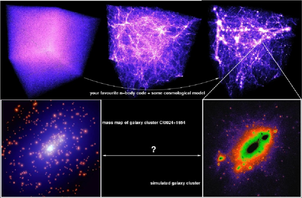
Figure 1: Illustration of the idea driving $N$-body simulations. Initial conditions are being evolved forward in time modeling gravity alone. The outputs over time are then compared to observational data and the cosmological model adjusted accordingly. Image credit (mass map of Cl0024+164): European Space Agency, NASA and Jean-Paul Kneib (Observatoire Midi-Pyrenees, France/Caltech, USA)

Figure 2: Initial conditions according to the Zeldovich approximation (cf. Eq. (1)). One clearly sees the decomposition of density perturbations as waves.

2 The Initial Conditions

The most common way to set up initial conditions for a cosmological simulation is to make use of the Zeldovich approximation to move particles from a Lagrangian point $\vec{q}$ to a Eulerian point $\vec{x}$ (e.g. Efstathiou et al. 1985):

$$\vec{x}=\vec{q}-D(t)\vec{S}(\vec{q})\ ,$$ (1)

where $D(t)$ describes the growing mode of linear fluctuations and $\vec{S}(\vec{q})$ is the ’displacement field’. The initial Lagrangian coordinates $\vec{q}$ are usually chosen to form a regular, three-dimensional lattice.

The displacement field $\vec{S}(\vec{q})$ is related to a pre-calculated input power spectrum of density fluctuations, $P(k)$, which in turn depends on the cosmological model under consideration

$$\vec{S}(\vec{q})=\nabla_{q}\Phi(\vec{q}),\ \ \ \Phi(\vec{q})=\sum_{\vec{k}}a_{\vec{k}}\cos(\vec{k}\cdot\vec{q})+b_{\vec{k}}\sin(\vec{k}\cdot\vec{q})\ ,$$ (2)

where the Fourier coefficients $a_{\vec{k}}$ and $b_{\vec{k}}$ are linked to $P(k)$ and are given as

$$a_{\vec{k}}=R_{1}\frac{1}{k^{2}}\sqrt{P(k)},\ \ \ b_{\vec{k}}=R_{2}\frac{1}{k^{2}}\sqrt{P(k)}.$$ (3)

$R_{1}$, $R_{2}$ are (Gaussian) random numbers with zero mean and dispersion unity.

An example for the Zeldovich approximation “at work” can be found in Fig. 2 where a slice through the initial conditions for a standard $\Lambda$CDM simulations at redshift $z=50$ is shown. This figure nicely demonstrate the decomposition of the density perturbations as waves.

3 Solving Poisson’s Equation

When used to model the dynamics of a collisionless system such as dark matter, an $N$-body code aims at simultaneously solving the collisionless Boltzmann equation (CBE)

$$\frac{\partial f}{\partial t}+\sum_{i=1}^{3}\left(v_{i}\frac{\partial f}{\partial x_{i}}-\frac{\partial\Phi}{\partial x_{i}}\frac{\partial f}{\partial v_{i}}=0\right)$$ (4)

and Poisson’s equation

$$\nabla^{2}\Phi(\vec{r})=4\pi G\rho(\vec{r})\ .$$ (5)

The CBE Eq. (4) is solved by the method of characteristics (e.g., Leeuwin, Combes & Binney 1993). Since the CBE states that $f$ is constant along any trajectory $\{\vec{r}(t),\vec{v}(t)\}$, the trajectories obtained by time integration of $N$ points $\{\vec{r}_{i},\vec{v}_{i}\}$ sampled from the distribution function $f$ at time $t=t_{\rm initial}$ form a representative sample of $f$ at each time $t$.

Hence the problem reduces to solving Poisson’s Eq. (5) for a set of $N$ particles and advancing them forward in time according to the equations of motion derived from the system’s Hamiltonian $H$ (remember that Eq. (4) can be written as $\partial f/\partial t+[f,H]=0$). The details of the time-integration of the equations of motions are going to be explained later on in Section 4 though; in this Section I like to focus on the gravity solver.

Currently there are two commonly used approaches for deriving the potential from Poisson’s equation: a) tree codes rely on a direct particle-particle summation, and b) PM (particle-mesh) codes utilize a numerical integration of Eq. (5) on a grid.

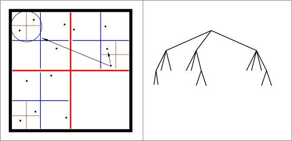
Figure 3: Illustration of a tree code. The left panel shows the actual particle distribution and its cubical decomposition. The right panel is the tree corresponding to this distribution.

3.1 Tree Codes

3.1.1 The Pre-Requisites

The particle-particle (PP) method upon which tree codes are based assumes that the particles are $\delta$-functions and hence the density field (rhs of Poisson’s equation Eq. (5)) reads as follows:

$$\rho(\vec{r})=\sum_{i=1}^{N}m_{i}\delta(\vec{r}-\vec{r}_{i})\ ,$$ (6)

where $N$ is the total number of particles in use.

3.1.2 The Forces

Combining Eq. (6) with Eq. (5) the analytical solution for the force $\vec{F}$ at particle position $\vec{r}_{i}$ is given by:

$$\vec{F}(\vec{r}_{i})=\sum_{j\neq i}\frac{m_{i}m_{j}}{|\vec{r_{i}}-\vec{r_{j}}|^{2}}\ .$$ (7)

But as we are interested in deriving the force at every single particle position, the PP method scales like $N^{2}$ ($N$ summations, each over $(N-1)$ particles). Therefore, a (straightforward) PP summation appears not to be feasible for evolving a set of $N$ particles under their mutual gravity, not even on the largest supercomputers available nowadays! One needs to bypass the increase in computational time for large numbers of particles with a more sophisticated treatment when calculating the forces. One way of achieving this is to organize the particles in a tree-like structure: particles located ”far away” from the actual particle (at which position we intend to calculate the force) can be lumped together as a single – but more massive – particle. This tunes down the number of calculations dramatically.

The idea of a tree code is sketched in Fig. 3. The particles are organized in a tree-like structure based upon a cubical decomposition of the computational domain. Consequentially, for each particle we “walk the tree” and add the forces from branchings that need no further unfolding into finer branches according some pre-selected “opening criterion”.

One publicly available tree code is called GADGET (Galaxies with Dark Matter and Gas intEracT) and I refer the reader to a more elaborate discussion of this technique to its reference paper by Springel, Yoshida & White (2001).

3.1.3 Force Resolution

In order to avoid the singularity for $\vec{r}_{i}=\vec{r_{j}}$ in Eq. (7) one needs to set a limit on the minimal allowed spatial separation between two particles. This can be achieved by introducing a (fixed) scale, i.e. the softening parameter $\epsilon$:

$$\vec{F}(\vec{r}_{i})=\sum_{j\neq i}\frac{m_{i}m_{j}}{|\vec{r_{i}}-\vec{r_{j}}|^{2}+\epsilon^{2}}$$ (8)

This softening is closely related to the overall force resolution of the simulation and an elaborate discussion of it can be found in Dehnen (2001).

3.2 Particle-Mesh Codes

3.2.1 The Pre-Requisites

Another way for obtaining the forces is to numerically integrate Poisson’s equation (5). This method, however, demands the introduction of a grid in order to define the density and hence the name particle-mesh (PM) method. The grid is usually of a regular (cubic) shape with $L\times L\times L$ cells where each cell is identified by the index triplet $(i,j,k)$. The forces are then calculated according to the following scheme:

1. assign all particles to the grid to get $\rho_{i,j,k}$

2. solve Poisson’s equation $\nabla^{2}\phi_{i,j,k}=4\pi G\rho_{i,j,k}$

3. differentiate to get forces $F_{i,j,k}=-\nabla\phi_{i,j,k}$

4. interpolate $F_{i,j,k}$ back to particle positions

3.2.2 The Forces

With this scheme most of the time is spent in step 2 and the most common way to solve Poisson’s equation on a grid is to make use of FFT’s (Fast-Fourier-Transforms). The analytical solution to Poisson’s equation is given by the integral

$$\Phi(\vec{r})=\int G(\vec{r}-\vec{r}^{\prime})\rho(\vec{r}^{\prime})d\vec{r}^{\prime}$$ (9)

where $G(\vec{x})=-\vec{x}/x^{3/2}$ is the Green’s function of Poisson’s equation. This integral can readily be evaluated in Fourier-space, i.e.

$$\hat{\Phi}=\hat{G}\ \hat{\rho}$$ (10)

where $\hat{\Phi}$, $\hat{G}$, and $\hat{\rho}$ are the Fourier transforms of the respective variables.

The PM approach proves to be exceptionally fast outperforming any tree code.

There are of course other techniques than the use of FFT’s available to numerically solve Poisson’s equation but the utilisation of FFT’s is the most common approach as it appears to be the fastest.

3.2.3 Force Resolution

The most severe problem with the PM method is the lack of spatial resolution below two grid spacings. Whereas tree codes require the introduction of a softening length to avoid the force singularity for close encounters of particles PM codes suffer from the opposite problem. Gravity is an attractive force and hence the particles flow from low density regions into high density regions amplifying primordial density fluctuations. This leads to an excess of particles in certain cells whereas other cells are becoming more and more devoid of matter. But as the spacing of the grid introduces a (smoothing) scale particles closer than about two cell distances do not interact according to Eq. (9) anymore. While we had to introduce a force softening for tree codes to avoid two-body interactions and make the simulation collisionless, respectively, the PM method naturally admits such a smoothing. However, we are left with the situation where we can not resolve structure formation on scales of (and below) roughly the cell spacing of the grid!

This is a major problem and the most obvious way to overcome it is to introduce finer grids in regions of high density. These grids though need to freely adapt to the actual particle distribution at all times and hence navigating such complex grids through computer memory is a very demanding task. One of the freely available adaptive mesh refinement (AMR) codes is MLAPM (Knebe, Green & Binney 2001).

The mode of operation of this AMR technique can be viewed in Fig. 4 where a slice through a standard $\Lambda$CDM simulation is presented. The left panel shows the distribution of particles whereas the right panel indicates the adaptive meshes used to obtain a solution to Poisson’s equation.

It needs to be stressed though that the use of irregularly shaped grids inhibits FFT’s. Another technique for solving Poisson’s equation needs to be sought such as, for instance, multi-grid relaxation (cf. Knebe, Green & Binney 2001).

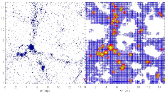
Figure 4: An example for adaptive mesh refinement. The left panel shows the particle distribution at redshift $z=0$ in a $\Lambda$CDM simulation. The right panel indicates the arbitrarily shaped grids invoked by the AMR code MLAPM to solve Poisson’s equation.

3.3 Hybrid Methods

There are, of course, various other techniques for simultaneously being time efficient and having a credible force resolution. One possibility is realized in the so-called P³M technique (i.e. Couchman 1991) where a combination of PP and PM provides the necessary balance between accuracy and efficiency: the force as given by the plain PM calculation is augmented by a direct summation over all neighboring particles within the surrounding cells. This gives accurate forces down to the scale provided by the softening parameter $\epsilon$ again. Other examples, for instance, are Tree-PM (Bode & Ostriker 2003) and moving mesh (Gnedin 1995) codes, but the details are well beyond the scope of this contribution.

3.4 Mass Resolution

It still needs to be mentioned that a cosmological simulation in practice only simulates a certain fraction of the Universe. This is what people refer to as the simulation box. However, to account for the fact the Universe is actually infinite one uses periodic boundary conditions: particles leaving the box on one side immediately enter the box again on the other side.

Moreover, the size of the box also defines the mass resolution of the simulation. We are only using a certain number of particles within a fixed region of the Universe. And as the density of the Universe is determined by the cosmological model under investigation, each individual particle has a certain mass. This mass determines the mass resolution of that specific simulation. For instance, if we model the evolution of about 2 million particles in a box with side length 25$h^{-1}{\ }{\rm Mpc}$ using the $\Lambda$CDM cosmology ($\Omega_{0}=0.3$), each particle weighs about $6\cdot 10^{8}$$h^{-1}{\ }{\rm M_{\odot}}$. Therefore we will not be able to resolve dwarf galaxies in that particular cosmological simulation ($M_{\rm dwarf}\geq 10^{7}$$h^{-1}{\ }{\rm M_{\odot}}$).

3.5 Comparison

It only appears natural to ask the question which method is superior and how they compare, respectively.

There is no straight forward answer as both methods have their (dis-)advantages. Tree codes are based upon the assumption that the Universe is filled with particles of a certain size related to the softening $\epsilon$ (cf. Section 3.1.3). Adaptive mesh refinement codes use a smoothed density field (which in turn also introduces an effective particle size) to obtain the potential and hence the force field. In both cases it is important to bear in mind that particles are only to be understood as markers in phase-space and should not interact on a two-body basis, i.e. one always intends to integrate the collisionless Boltzmann equation (4). There are several studies investigating two-body interactions in such simulations and it can be confirmed that they are more prominent in tree codes (Binney & Knebe 2002). But as long as one complies with certain constraints on the numerical parameters (cf. Power et al. 2003) such effects can be minimized.

There are several studies comparing tree and AMR codes both in efficiency and accuracy (cf. Frenck et al. 1999, Knebe et al. 2001, O’Shea et al. 2003) but in the end it all comes down to a “question of taste”. Both techniques are well enough developed to successfully model the formation and evolution of cosmic structures.

4 Newtonian Mechanics in an Expanding Universe

Even though solving Poisson’s equation is the heart and soul of every $N$-body code, it is also important to accurately update particle positions and velocities, i.e. integrating the equations of motion. And as the Universe is expanding it is convenient to introduce comoving coordinates:

$$\vec{x}=\vec{r}/a(t)\,$$ (11)

where $a(t)$ is the cosmic expansion factor.

The (comoving) Lagrangian is given by

$${\mathcal{L}}={\textstyle{1\over 2}}a^{2}\dot{x}^{2}-{\Phi\over a},$$ (12)

which leads to the canonical momentum

$$\vec{p}=a^{2}\dot{\vec{x}}.$$ (13)

Hamilton’s equations are therefore

$$\begin{array}[]{lcc}\displaystyle\frac{{\rm d}\vec{x}}{{\rm d}t}&=&\displaystyle{\vec{p}\over a^{2}}\\ \\ \displaystyle\frac{{\rm d}\vec{p}}{{\rm d}t}&=&\displaystyle-{\nabla\Phi\over a}\ .\end{array}$$ (14)

These equations can be discretized and integrated using a second-order accurate scheme as follows:

$$\vec{x}_{n+1/2} = \vec{x}_{n}+\vec{p}_{n}\int_{t}^{t+\Delta t/2}{{\rm d}t\over a^{2}}$$

$$\vec{p}_{n+1} = p_{n}-\nabla\Phi(x_{n+1/2})\int_{t}^{t+\Delta t}{{\rm d}t\over a}$$ (15)

$$\vec{x}_{n+1} = \vec{x}_{n+1/2}+\vec{p}_{n+1}\int_{t+\Delta t/2}^{t+\Delta t}{{\rm d}t\over a^{2}},$$

where the integrals can be evaluated analytically as they depend only on the cosmology.

This modified leap-frog scheme only needs to store one copy of the positions and velocities whereas other integrators as, for instance, Runge-Kutta consume more memory.

5 Final Remarks

A broad overview of the concepts behind cosmological $N$-body simulations has been presented. After a short introduction explaining the needs for such simulations I explained how to actually set up the initial conditions. There are numerous techniques for evolving that set of $N$ particles forward in time under the influence of its own self-gravity alone, but I focused on two (diverse) methods, namely tree codes and adaptive mesh refinement codes. Their mode of operation has been introduced and their limitations pointed out and compared with each other.

This contribution can only be understood as a very brief and general introduction to the ideas behind cosmological $N$-body simulations. It is far from being complete and exhaustive and I refer the reader to more elaborate review articles such as Bertschinger (1998) and the monograph “Computer Simulations using Particles” by Hockney & Eastwood (1988).

References

- (1) Aarseth S.J., 1963, MNRAS 126, 223
- (2) Bertschinger E., 1998, Ann. Rev. A & A 36, 599
- (3) Binney J.J., Knebe A., 2002, MNRAS 333, 378
- (4) Bode P., Ostriker J.P., 2003, ApJS 145, 1
- (5) Couchman H.M.P., 1991, ApJ 368, 23
- (6) Dehnen W., 2001, MNRAS 324, 273
- (7) Efstathiou G., Eastwood J.W., 1981, MNRAS 194, 505
- (8) Efstathiou G., Davis M., White S.D.M., Frenk C.S., 1985, ApJS 57, 241
- (9) Frenck C.S. et al. , 1999, ApJ 525, 554
- (10) Gill S.P.D., Knebe A., Gibson B.K., 2004, MNRAS 351, 399
- (11) Gnedin, N.Y., 1995, ApJS 97, 231
- (12) Hockney R.W., Eastwood J.W., Computer Simulations Using Particles, 1988, Bristol: Adam Hilger
- (13) Knebe A., Green A., Binney J.J., 2001, MNRAS 325, 845
- (14) Leeuwin F., Combes F., Binney J., 1993, MNRAS 262, 1013
- (15) O’Shea B.W., Nagamine K., Springel V., Hernquist L., Norman M.L., 2003, astro-ph/0312651
- (16) Peebles P.J.E., 1970, Astron. J. 75, 13
- (17) Power C., Navarro J. F., Jenkins A., Frenk C. S., White S. D. M., Springel V., Stadel J., Quinn T., 2003, MNRAS 338, 14
- (18) Springel V., Yoshida N., White S.D.M., 2001, NewA 6, 15