Tracing the Warm Hot Intergalactic Medium in the Local Universe

Abstract

We present a simple method for tracing the spatial distribution and predicting the physical properties of the Warm-Hot Intergalactic Medium (WHIM), from the map of galaxy light in the local universe. Under the assumption that biasing is local and monotonic we map the $\sim 2\ {\rm{\it h}^{-1}Mpc}$ smoothed density field of galaxy light into the mass density field from which we infer the spatial distribution of the WHIM in the local supercluster. Taking into account the scatter in the WHIM density-temperature and density-metallicity relation, extracted from the $z=0$ outputs of high-resolution and large box size hydro-dynamical cosmological simulations, we are able to quantify the probability of detecting WHIM signatures in the form of absorption features in the X-ray spectra, along arbitrary directions in the sky. To illustrate the usefulness of this semi-analytical method we focus on the WHIM properties in the Virgo Cluster region.

1 Introduction

As pointed out for the first time by Fukugita, Hogan and Peebles (1998) the census of baryons in the low redshift universe is significantly below expectations. Indeed, the baryon fraction detected in the Ly$\alpha$ forest at $z\sim 2$ (e.g. Rauch 1998), which agrees with the recent WMAP measurements of the Cosmic Microwave Background (Bennett et al. 2003), is more than a factor of 2 larger than that associated with stars, galaxies and clusters in the universe at $z\sim 0$ (Cen & Ostriker 1999).

Recent studies based on large box-size, hydro-dynamical simulations have suggested that a significant fraction of the baryons at $z\sim 0$ are found in a gaseous form, with a temperature between $10^{5}$ and $10^{7}$ K in regions of moderate overdensities $\delta\sim 10-100$ (Ostriker & Cen 1996; Perna & Loeb 1998; Cen & Ostriker 1999; Davé et al. 2001; Cen et al. 2001), hence providing a possible explanation to the missing baryons problem. This Warm-Hot Intergalactic Medium (WHIM) is found to be in the form of a network of filaments, and could be observed in the spectra of background bright sources in the X-ray and far-UV bands in the form of absorption lines due to elements in high ionization state, like OVI, OVII and OVIII (Hellsten et al. 1998, Tripp et al. 2000, Cen et al. 2001, Furlanetto et al. 2004).

The detection of WHIM, however, is challenging. To date the most significant detection ($>3\sigma$) in the X-ray band has been made in correspondence of an absorption line in the Chandra spectrum of the Blazar Mkn 421 that has been interpreted as due to two interviewing WHIM OVII systems at $z=0.011$ and $z=0.027$ and with column densities $\raise-2.0pt\hbox{\hbox to0.0pt{\hbox{$\sim$}\hss}\raise 5.0pt\hbox{$>$}\ }8\times 10^{14}$ cm^-2 (Nicastro et al. 2004). Fang et al. (2002) have reported a detection of an OVIII absorption line along the sight-line toward PKS 2155-304 with Chandra at $z>0$ that, however, has not been confirmed by subsequent observations performed with XMM-Newton. The identification of the absorbers in the very local universe with WHIM structures in the local group/supercluster is even more controversial (Nicastro et al. 2003, Savage et al. 2003). Finally, emission by the WHIM could also be important and some detections have been claimed, either by observing X-ray excess in clusters of galaxies (e.g. Kaastra et al. 2003) or by observing soft X-ray structures associated with galaxy overdensities (Zappacosta et al. 2004).

Although these observations are very encouraging and seem to indicate that we have just started to detect the WHIM, various problems are still preventing us from a detailed investigation of its properties.

First of all, the detection of WHIM is particularly difficult and requires very sensitive UV and X-ray detectors, both for absorption and for emission processes. With the presently available instruments, the WHIM absorption lines can only be detected in very high signal-to-noise spectra either obtained with very long exposures of bright extragalactic sources or by observing variable sources like Blazars when they undergo an outburst phase. In either case, expected detections will be so rare that a detailed study of the WHIM will have to wait for future observations by next generation X-ray satellites such as XEUS and Constellation-X (Chen et al. 2003, Viel et al. 2003).

The second issue, on which we will focus in this work, is the difficulty in modeling the WHIM. Hydro-dynamical simulations of structure formation in the context of cold dark matter models have certainly provided a major contribution to the understanding of the physics of the WHIM and to the characterizing its spatial distribution. However, in general, they are not designed to model the actual WHIM distribution in our universe, i.e. they do not tell us where we should look for the WHIM in our cosmic neighborhood. The hydro-dynamical simulations of Kravtsov et al. (2002) and, more recently of Yoshikawa et al. (2004), constitute the only attempt to model the gas distribution in the Local Supercluster region to address WHIM detectability. The simulations by Kravtsov et al. (2002) make self-consistent use of constraints from the MARK III catalog of galaxy peculiar velocity to reproduce the large-scale mass density field within $\sim 100\ {\rm{\it h}^{-1}Mpc}$, including major nearby structures like the Local Group, the Local Supercluster, Virgo and Coma clusters (Klypin et al. 2003). However, their peculiar velocity constraints are only effective above a (Gaussian) resolution scale $>5\ {\rm{\it h}^{-1}Mpc}$ which is significantly larger than the typical widths of the WHIM structures (Viel et al. 2003). The constraints of Yoshikawa et al. (2004) are derived from the redshift space positions of IRAS 1.2Jy galaxies and are effective on a $5\ {\rm{\it h}^{-1}Mpc}$ Gaussian scale. As a consequence, in both models the actual position of the WHIM absorber within the resolution element of a single numerical simulation is essentially random. A large number of constrained hydro-dynamical simulations, characterized by independent sets of Fourier modes on sub-resolution scales, would then be required to produce independent realizations of the intergalactic gas in the local universe from which a probability of detecting a WHIM absorber at a given spatial location can be computed.

Unfortunately, this approach is too time-consuming to be successfully implemented using hydro-simulations and to allow an accurate study of all the possible physical processes which can influence the properties of the WHIM at $z\sim 0$ such as the effect of different amount of feedback in the form of galactic winds, the distribution of metals and the effect of having different temperature-density relations.

For this reason we have developed an alternative semi-analytical modeling, still based on the same probabilistic approach, in which we use the existing results of hydro-dynamical simulations at $z=0$ to trace the intergalactic gas from the spatial distribution of galaxy light in the local supercluster. The intrinsic scatter in the gas vs. galaxy light relation is accounted for by performing independent realizations of the gas distribution in the local universe which we can produce by means of fast Montecarlo techniques. Another advantage of our method is that our constraints, that derive from mapping the galaxy light, apply down to scales of $\sim 1\ {\rm{\it h}^{-1}Mpc}$, comparable to the width of WHIM structures and much smaller than the galaxy correlation length, hence allowing us to trace the local WHIM with higher resolution. Obviously, these considerations are valid as long as light to gas mapping is local and well modeled by our reconstruction technique, which we will show is indeed the case.

The outline of the paper is as follows. In Section 2 we will describe the galaxy catalog used in our analysis. Section 3 presents the hydro-dynamical cosmological simulations used to model the WHIM structures. In Section 4 we will describe the method to produce X-ray absorption spectra along an arbitrary direction in the sky starting from the galaxy luminosity map in the local universe and from the physical properties of WHIM structures as extracted from the hydro-dynamical simulations. Section 5 contains a testing of the modeling, while an application to the local universe is presented in Section 6. Section 7 contains our conclusion and the future developments of the method proposed.

2 The Nearby Galaxy Luminosity Field

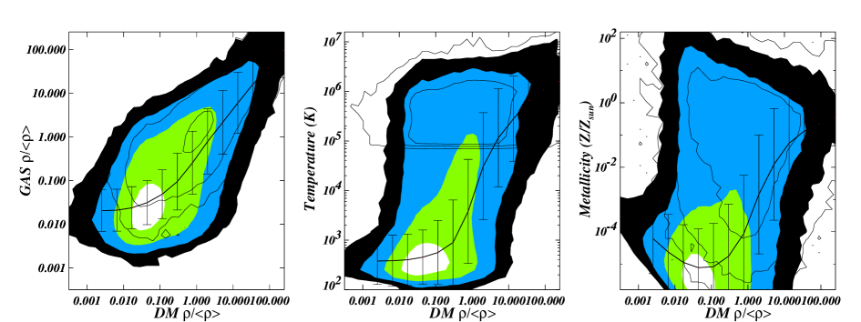
Figure 1: Left panel: Gas density as a function of mass density (in units of the mean density) as extracted from the $z=0$ output of a $\Lambda$CDM simulation with a box size of $25\ {\rm{\it h}^{-1}Mpc}$ (our fiducial simulation, see Section 3). The line represents the median value in each bin and error bars are the $1\,\sigma$ values. Filled contour plots represent the number density of points in the simulation (number density increases by an order of magnitude at each contour level). The empty contours show the number density of those pixels with $T>10^{5}$ K (number density increases by an order of magnitude at each contour level). Central panel: Gas temperature as a function of mass density. Right panel: Gas metallicity (in units of solar metallicity) as a function of mass density.

The galaxy sample considered in this work has been extracted from the latest version of the Nearby Galaxies Catalog (Tully 1988). The extraction is a cube with cardinal axes in supergalactic coordinates that extend to $\pm 1500$ km s^-1, centered on our Galaxy. This boundary fully encompasses the Virgo, Ursa Major, Coma I, and Fornax clusters. The database strives for completeness among all galaxy types known. The all-sky optical surveys accumulated in ZCAT (http://cfa-www.harvard.edu/$\sim$huchra/zcat/zcom.htm) provides completeness at all but low galactic latitudes for high surface brightness galaxies. Though dated, the HI survey of Fisher and Tully (1981) provides the most complete all-sky coverage of low surface brightness irregular galaxies. The catalog lists angular positions, redshifts, and B-band luminosities. There has been compensation for the small incompleteness associated with the zone of avoidance through the addition of fake sources through reflection of real sources at higher latitudes. In total, the catalog contains 1968 real sources and 106 fake sources within the cube of diameter 3000 km s^-1. There is correction for missing information with distance but it is very small. The information to be used is the luminosity density at B-band (not the galaxy number density). The sample has a faint luminosity clip at $M_{B}=-16+5{\rm log~{}H}_{0}/100$. The catalog is essentially complete for galaxies of this luminosity at the boundaries of the cube along the cardinal axes. Corrections for lost light amount to 30% at the far corners of the cube.

The analysis to be discussed is performed in real rather than redshift space. The finger of god velocities in clusters have been collapsed so the clusters have depths comparable to their projected dimensions. Then distances have been assigned to groups and individual galaxies in accordance with the output of a Least Action Model (Peebles 1989; Shaya, Peebles, and Tully 1995) constrained by 900 individual distance measurements. This model provides a reasonable description of galaxy flows in the neighborhood of the Virgo Cluster.

3 Hydro-dynamical simulations

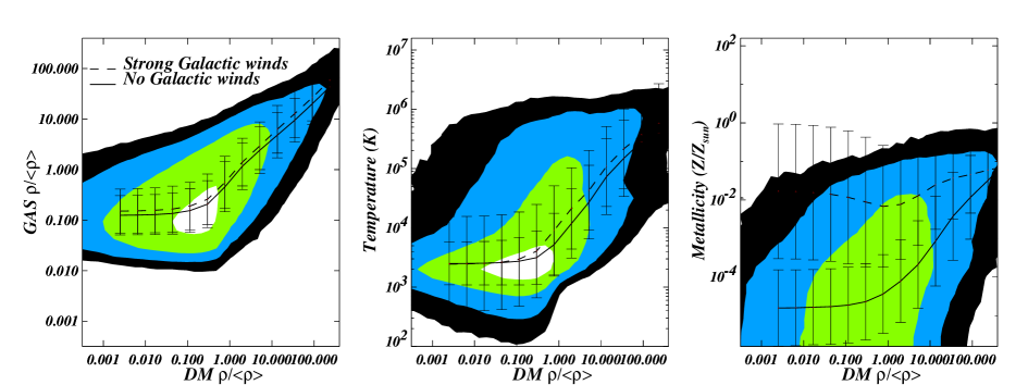
Figure 2: Left panel: Gas density as a function of mass density (in units of the mean density) as extracted from the $z=0$ output of a $\Lambda$CDM simulation of $11\ {\rm{\it h}^{-1}Mpc}$ (see Section 3 and Cen, Nagamine, Ostriker 2004 for more details). The lines represent the median value in each bin and error bars are the $1\,\sigma$ values. The continuous lines in all the panels refer to a simulation without galactic winds while the dashed ones are for a simulation with strong galactic superwinds. Filled contour plots represent the number density of points in the simulation without galactic winds (number density increases by an order of magnitude at each contour level). Central panel: Gas temperature as a function of mass density. Right panel: Gas metallicity (in units of solar metallicity) as a function of mass density.

The fiducial hydro-dynamical simulation used here is a $\Lambda$CDM model with the following parameters: $H_{0}=100h$ km s^-1Mpc^-1 with $h=0.67$, $\Omega_{0m}=0.30$, $\Omega_{0b}=0.035$, $\Omega_{\Lambda}=0.70$, $\sigma_{8}=0.90$, and the spectral index of the primordial power spectrum $n=1$. The box-size of the simulation is $25\ {\rm{\it h}^{-1}Mpc}$ comoving on a uniform mesh with $768^{3}$ cells. The comoving cell size is 32.6 $h^{-1}$ kpc and the mass of each dark matter particle is $\sim 2\times 10^{7}$ M_⊙ (further details can be found in Cen et al. 2003). The simulation includes galaxy and star formation, energy feedback from supernova explosions, ionization radiation from massive stars and metal recycling due to SNe/galactic winds. Metals are ejected into the local gas cells where stellar particles are located using a yield $Y=0.02$ and are followed as a separate variable adopting the standard solar composition. This simulation can be considered a good compromise between box size and resolution to investigate the WHIM properties (see discussion in Cen et al. 2001).

The X-ray and UV background of the simulation at $z=0$, which are needed to properly simulate X-ray absorptions, are computed self-consistently from the sources in the simulation box. We have checked that there are very small differences between the hydro-simulation background and the estimate from Shull et al. (1999): $I_{UV}=I_{UV}^{0}(E/13.6\rm{eV})^{-1.8}$, with $I_{UV}^{0}=2.3\times 10^{-23}$ erg cm^-2 Hz^-1 sr^-1 s^-1 for the UV background (which includes a contribution from AGNs and starburst galaxies), and $I_{X}=I_{X}^{0}(E/E_{X})^{-1.29}\exp{(-E/E_{X})}$, with $I_{X}^{0}=1.75\times 10^{-26}$ erg cm^-2 Hz^-1 sr^-1 s^-1 and $E_{X}=40$ keV (Boldt 1987; Fabian & Barcons 1992; Hellsten et al. 1998; Chen et al. 2003), for the X-ray background. The difference between the amplitude of the UV and X-ray background of the hydro-simulations and the estimates above is less than a factor of 2, in the range 0.003 $\sim$$<$ E (keV) $\sim$$<$ 4. Among the two backgrounds, the X-ray one plays a major role in determining the statistics of the simulated spectra. We will assume that the amplitude of the ionizing backgrounds scales like $(1+z)^{3}$, in the redshift range $0<z<1$ (this is in agreement with the evolution of the radiation field in the simulation). This assumption will not influence significantly our results: given the fact that we will generate mock-spectra at $z\sim 0$.

Along with the ionizing background, the other quantities extracted from the hydro simulations which are relevant for our work are the mass density, and the density, temperature and metallicity of the gas. All these quantities have been re-binned on a coarser $256^{3}$ cubic grid, with cells of comoving size 97.6 $h^{-1}$ kpc. In the rest of the paper we will label as fiducial the simulation with a box of 25 $h^{-1}$ comoving Mpc and $768^{3}$ cells rebinned into a mesh of $256^{3}$. In the following we will refer to these quantities as the unsmoothed fields and will indicate them with the upper index ${\rm U}$.

The gas density-mass density relation in the hydro-dynamical simulation is shown by the contour plot in the left panel of Figure 1, where we also report the median value in each density bin (continuous line) and the rms values. Similarly, the central and right panels show the gas temperature and gas metallicity as a function of mass density, The filled contour plots represent, in all panels, the number density of mass density elements in a given bin of gas-density/mass-density, gas-temperature/mass-density and gas-metallicity/mass-density in the hydro-dynamical simulation. The empty contours represent the number density of gas elements with $T>10^{5}$K, i.e. the gas effectively responsible for absorption. We prefer to show these plots instead of the usual gas density-temperature and gas density-metallicity relation (as in Viel et al. 2003), because our modeling starts from the mass distribution and uses these relations to predict the WHIM distribution and properties.

The relations shown in Figure 1 are in reasonable agreement with the recent results obtained by Yoshida et al. (2002 - their Figure 2) and also by Davé et al. (1999), who studied the gas cooling processes in the framework of Smoothed Particle Hydro-dynamics (SPH) simulations. We note that the scatter in temperature can be very high for values of $\log(1+\delta_{\rm m}^{\rm U})>-1$, spanning more than one order of magnitude. The mass density-metallicity relation in the right panel is as expected: low density regions are the most metal poor, while at large densities the metallicity can be solar. In this plot the scatter is extremely large for the intermediate density regime, i.e. $-1<\log(1+\delta_{\rm m}^{\rm U})<0.5$, while it is significantly smaller for larger overdensities. This plot has to be compared with similar plots shown in Cen & Ostriker (1999b), but here we find that the scatter is somewhat larger than in previous simulations. This can be due to the different amount of feedback in the hydro-simulation. The effect of feedback on WHIM structures will be investigated in a future work.

However, to have a first hint on what properties of the WHIM are sensitive to the physics implemented into the hydro-dynamical simulations we have analyzed the $z=0$ of two other simulation with a smaller box size and at higher resolution. These simulations have a box size of $11\ {\rm{\it h}^{-1}Mpc}$ comoving on a uniform mesh of 432³ elements and with the following cosmological parameters: $\Omega_{0m}=0.29,\Omega_{0b}=0.047,\Omega_{\Lambda}=0.71,\sigma_{8}=0.85,n=1,h=0.7$, and are extensively described in Cen et al. (2003) and Cen, Nagamine & Ostriker (2004). The main difference between this second set of simulations and our fiducial one relies in the presence of galactic superwinds. These are generated as feedback from star formation and are normalized to match Lyman Break galaxies observations. In Figure 2 we plot the gas density, the gas temperature and the gas metallicity vs. dark matter density relations as in Figure 1. We note that, while the gas density-dark matter density relation is very similar, the temperature plot and the metallicity one show some differences. In particular, it seems that at a fixed density the temperature of the gas is about a factor two smaller than in the larger box size one. This can be determined both by the different feedback implementations and by the smaller box size which samples a volume which is certainly not large enough to contain massive structures. Another major difference is in the metallicity-dark matter density diagram, where one can see that in the case of strong galactic winds, represented by the dashed line, the low density regions are significantly metal enriched. For the higher density regions with $10<\delta<100$ the discrepancy is smaller but still it seems that in the presence of galactic winds their metallicity can be a factor $\raise-2.0pt\hbox{\hbox to0.0pt{\hbox{$\sim$}\hss}\raise 5.0pt\hbox{$<$}\ }2$ higher than in the no winds case. This is a very similar trend to that found by Cen, Nagamine & Ostriker (2004) at higher redshift in the Lyman$-\alpha$ forest and shows that winds are effective in polluting the low density intergalactic medium with metals. Another feature which is worth stressing is the fact that both the temperature-dark matter density and the metallicity-dark matter density relations in the simulation with winds show larger scatter (about a factor two) when compared to the simulations without winds. The results with no winds (continuous line) are however in reasonable good agreement with our fiducial simulation ( Figure 1), which contains a different and probably less effective implementation of feedback by galactic winds.

In this Section we have analyzed the properties of the WHIM as derived from hydro-dynamical simulations with different box-sizes and different implementation of physical processes. Among all the effects we found that the presence of galactic winds and the box sizes are important in determining the properties of the WHIM in particular its temperature and metallicity. In the semi-analytic modeling we are going to propose in the following Sections, which is of course less accurate than the hydro-dynamical simulations described here, an implementation of the different relations shown in Figures 1 and 2 will be straightforward, allowing us to produce many realizations of the local universe WHIM distribution.

4 From Galaxy Light to WHIM

In this Section we describe a method to infer the spatial distribution of the Intergalactic Medium from the observed galaxy distribution in the local universe. The method consists of four steps, described in the next sub-sections, through which the B-band luminosity density field obtained from the Tully catalog is used to infer the spatial distribution of the dark matter. Then, from the dark matter density field we predict the spatial distribution, temperature and metallicity of the intergalactic gas in the local universe.

4.1 Light to Smoothed Mass Mapping

To map the observed light distribution into the mass distribution we have applied the inversion method of Sigad, Branchini and Dekel (2000). As pointed out by Dekel and Lahav (1999) the relation between two random fields like $\delta_{\rm L}$ and $\delta_{\rm m}$, can be described by the conditional probability distribution $P(\delta_{\rm m}|\delta_{\rm L})$. If this relation were deterministic, then the relation between the two fields would be completely specified by the mean biasing function

$$\langle\delta_{\rm m}|\delta_{\rm L}\rangle=\int P(\delta_{\rm m}|\delta_{\rm L})\delta_{\rm m}d\delta_{\rm m}\;.$$ (1)

Under the hypothesis that the relation between $\delta_{\rm L}$ and $\delta_{\rm m}$ is deterministic and monotonic then the mean relation $\langle\delta_{\rm m}|\delta_{\rm L}\rangle$ can be obtained by equating the cumulative distribution of $\delta_{\rm L}$, $C_{\rm L}(\delta_{\rm L})$, and $\delta_{\rm m}$, $C_{\rm m}(\delta_{\rm m})$, at given percentiles:

$$\langle\delta_{\rm m}|\delta_{\rm L}\rangle=C^{-1}_{\rm m}[C_{\rm L}(\delta_{\rm L})]\ ,$$ (2)

where $C^{-1}_{\rm m}$is the inverse function of $C_{\rm m}$.

In general, however, the relation is not deterministic since the value of the $\delta_{\rm L}$ at a generic location might not be solely determined by $\delta_{\rm m}$. In fact, other physical quantities, such as the gas temperature, or for example local shear, affect the process of galaxy formation and evolution (e.g. Blanton et al. 1999) and thus can introduce a scatter in the relation usually referred to as stochasticity. In presence of stochasticity, $C_{\rm m}^{-1}[C_{\rm L}(\delta_{\rm L})]$ may still be a good approximation for $\langle\delta_{\rm m}|\delta_{\rm L}\rangle$ as long as the biasing is monotonic. Branchini et al. (2004) applied this method to the simulation of Cen et al. (2001) to test the validity of this approach. More precisely, they have estimated the mean biasing relation from the cumulative distribution function of the $\sim 2\ {\rm{\it h}^{-1}Mpc}$-smoothed density fields of galaxy light and mass in the hydrodynamical simulation. They found that the $\langle\delta_{\rm m}|\delta_{\rm L}\rangle$ measured in the simulation agrees well with its estimate, $C_{\rm m}^{-1}[C_{\rm L}(\delta_{\rm L})]$, within the errors.

The method has been implemented as follows. First we have considered the luminosity overdensity field at the generic grid point position, $\delta_{\rm L}^{\rm S}(\bf{x})$, and have assigned a mass overdensity $\delta_{\rm m}^{\rm S}(\bf{x})$ $=C_{\rm m}^{-1}[C_{\rm L}(\delta_{\rm L}^{\rm S}(\bf{x}))]$. The result is a mean mass overdensity field that we have perturbed by adding a Gaussian scatter that accounts for both the stochasticity and the uncertainties affecting the determination of $\langle\delta_{\rm m}|\delta_{\rm L}\rangle$. A detailed study of the mean biasing function of the B-band galaxy light density of the Tully catalog will be presented by Branchini et al. (2004). Here, we only stress that the resulting biasing function is monotonic, i.e. it satisfies the main requirement of the light to mass mapping procedure, and is in good agreement with the mean B-band light biasing function measured in the hydrodynamical simulation of Cen et al. (2001), once that sampling errors and cosmic scatter are accounted for.

Using the mean biasing function measured by Branchini et al. (2004) and an estimate of the scatter around the mean obtained from the hydrodynamical simulation, we have applied our mapping procedure to the observed B-band galaxy light map and have obtained 30 different realizations of the mass density field in the local universe that will constitute one of the input of the reconstruction procedure presented in this work.

Figure 3: Left: The one point probability distribution function for the original lognormal density field extracted from hydro-dynamical simulation $\delta_{\rm LN}$ (continuous line); for the same field smoothed with a Top Hat filter of radius $2500\ {\rm km\,s^{-1}}$ (dashed line); for the reconstructed density field, $\delta_{\rm m}^{\rm SRR}$ (open squares) and for the reconstructed field smoothed on the same scale (filled triangles). Right: Power spectra of the same four density fields, characterized by the same symbols/line-styles.

4.2 Smoothed Mass to Unsmoothed Mass Mapping

The mass field $\delta_{\rm m}^{\rm S}$ obtained from the light distribution is smoothed on a Gaussian scale $r_{s}=95\ {\rm km\,s^{-1}}$ which is too large to investigate the properties of the X-ray absorbers in the local universe.

The problem of how to infer an unsmoothed mass density field, $\delta_{\rm m}^{\rm U}$, from a smoothed one, i.e. how to recover the correlation properties on sub-resolution scale from large scales constraints, is well known. A self-consistent solution is found when $\delta_{\rm m}^{\rm U}$ is Gaussian and the power spectrum of mass density fluctuations is known a priori (Hoffman & Ribak 1991). Unfortunately, in our case the nonlinear evolution has caused both $\delta_{\rm m}^{\rm U}$ and $\delta_{\rm m}^{\rm S}$ fields to deviate from Gaussianity and we cannot use conventional reconstruction techniques.

Therefore, we have developed an alternative reconstruction strategy that only assumes a priori knowledge of the mass power spectrum which we set to be the same as in the hydro-simulation discussed in Section 3. This method consists of two steps:

${\it i)}$ We start from any of the 30 realizations of $\delta_{\rm m}^{\rm S}$ and increase the power on sub-resolution scales by adding Fourier modes with random phases for wavenumbers larger than $k_{S}=2\pi/r_{S}$ in such a way to follow the power spectrum of the hydro simulations and to preserve the original spectral shape and amplitude on wavenumbers larger than $k_{S}$. Motivated by the fact that the one point probability distribution function [PDF] of $\delta_{\rm m}^{\rm U}$ should be close to lognormal we add the power on the lognormal field $\delta_{\rm LN}^{\rm U}\equiv{\rm ln}(1+\delta_{\rm m}^{\rm U})/<{\rm ln}(1+\delta_{\rm m}^{\rm U})>-1$ rather than to $\delta_{\rm m}^{\rm U}$. We label the new mass density field as $\delta_{\rm m}^{\rm SR}$ to indicate that random power has been added to the smoothed field on sub-resolution scales.

${\it ii)}$ At this point, we enforce the correct mass PDF by performing rank ordering between $\delta_{\rm m}^{\rm SR}$ and the mass density field extracted from the hydro-simulation, $\delta_{\rm m}^{\rm U}$. We indicate the resulting mass density field as $\delta_{\rm m}^{\rm SRR}$.

The whole purpose of this SRR reconstruction procedure is to obtain an unsmoothed density field, $\delta_{\rm m}^{\rm SRR}$, with a power spectrum that resembles that of the original hydro-dynamical simulations over the whole range of wavenumbers and possesses the same PDF of $\delta_{\rm m}^{\rm U}$. It is worth stressing that this procedure is not self-consistent and therefore we do not expect to reconstruct the original mass density field on a point-by-point basis. However, as we will show in the next section, this reconstruction method works reasonably well in regions of enhanced density where the warm hot phase of the intergalactic gas typically resides.

4.3 Mass to Intergalactic Gas Mapping

As a further step we map the mass overdensity field, $\delta_{\rm m}^{\rm SRR}$, into gas overdensity, temperature and metallicity. We do that by using the relations between these quantities determined from the hydro simulation described in Section 2 and displayed in Figure 1. The large scatter in these plots is highly non Gaussian. As a consequence we cannot assign any of the gas properties as a Gaussian deviate about the mean value of the gas density, temperature and metallicity measured in each mass density bin. Instead, we take the number of elements in each bin of the contour plots shown in Figure 1 to be proportional to the joint probability of any two quantities, for example, $(\delta_{\rm gas},\delta_{\rm m}^{\rm U})$, and assign the gas properties ($\delta_{\rm gas},{\rm T}_{\rm gas}$ and ${\rm Z}_{\rm gas}$) to the generic mass element by Montecarlo sampling each of the joint probability functions $P(\delta_{\rm gas},\delta_{\rm m}^{\rm U})$, $P({\rm T}_{\rm gas},\delta_{\rm m}^{\rm U})$, and $P({\rm Z}_{\rm gas},\delta_{\rm m}^{\rm U})$,.

This allows us to infer the spatial distribution of the Intergalactic Medium (IGM) in the local universe that is guaranteed to reproduce the correct one point PDF of the density, temperature and metallicity of the gas in the hydro-simulation. We stress that in the simple modeling presented here an implementation of different metallicity-temperature relations, motivated by physical arguments, will be straightforward.

It is worth noting that Montecarlo sampling of the probability distribution function is an approximate procedure that has the advantage of being easy to implement. However, the large scatter introduced by this procedure, that reflect the one present in the probability functions, may spoil our ability to reconstruct the properties of the X-ray absorbers. We will check below if this is indeed the case.

4.4 Intergalactic Gas to X-ray Absorbers Mapping

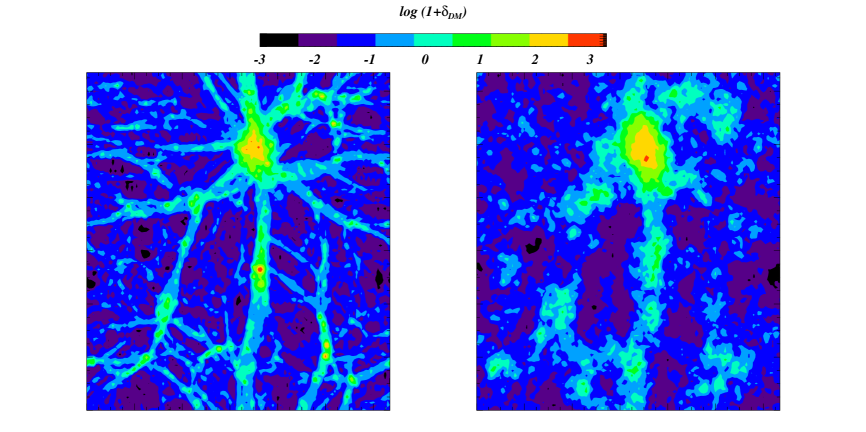
Figure 4: Left : The mass density field on a slice of $25\times 25\times 0.2\ {\rm{\it h}^{-1}Mpc}$ around the most massive object found in the hydro-dynamical simulation. Right: The reconstructed dark matter density field $\delta_{\rm m}^{\rm SRR}$ in the same region. The most massive structures at the typical overdensities of WHIM are preserved.

After having simulated the gas distribution, the photoionization code CLOUDY (Ferland et al. 1998) is used to compute the ionization states of metals, taking into account the UV and X-ray background. The density of each ion is obtained through: $n_{I}(x)=n_{H}(x)X_{I}Y_{Z_{\odot}}Z/Z_{\odot}$, where $X_{I}$ is the ionization fraction of the ion as determined by CLOUDY and depends on gas temperature, gas density and ionizing background, $n_{H}$ is the density of hydrogen atoms, Z is the metallicity of the element and $Y_{Z_{\odot}}$ is the solar abundance of the element.

Among the heavy elements that can produce absorption lines in the X-rays Oxygen is the most abundant one and produces the strongest lines. In this work we only simulate absorption spectra for the two strongest transitions of the ions OVII ($E=0.57$ keV, $\lambda=21.6\AA$, $f=0.7$) and OVIII ($E=0.65$ keV, $\lambda=18.97\AA$, $f=0.42$), with $f$ the oscillator strength. As pointed out by Viel et al. (2003), in the temperature and density range typical of WHIM, these two ions have a recombination time smaller that the Hubble time and thus the approximation of photoionization equilibrium should be reasonable.

Given the density of a given ion along the line-of-sight, the optical depth in redshift-space at velocity $u$ (in km s^-1) is

$$\tau_{I}(u)={\sigma_{0,I}c\over H(z)}\int_{-\infty}^{\infty}dy\,n_{\rm I}(y){\cal V}\left[u-y-v_{\parallel}^{\rm I}(y),b(y)\right]$$ (3)

where $\sigma_{0,I}$ is the cross-section for the resonant absorption and depends on $\lambda_{I}$ and $f_{I}$, $y$ is the real-space coordinate (in km s^-1), ${\cal V}$ is the standard Voigt profile normalized in real-space, $b=(2k_{B}T/m_{I}c^{2})^{1/2}$ is the thermal width and we assume that $v_{I}=v_{IGM}$ is the peculiar velocity. Velocity $v$ and redshift $z$ are related through $d\lambda/\lambda=dv/c$, where $\lambda=\lambda_{I}(1+z)$. For the low column-density systems considered here, the Voigt profile is well approximated by a Gaussian: ${\cal V}=(\sqrt{\pi}b)^{-1}\exp[-(u-y-v_{\parallel}^{\rm I}(y))^{2}/b^{2}]$. The X-ray optical depth $\tau$ will be the sum of the source continuum, which we assume we can determine, and that of eq. (3). Finally, the transmitted flux is simply ${\cal F}=\exp(-\tau)$.

5 Testing the modelling

In this Section we use the hydro simulation described in Section 3 to test the ability of our reconstruction procedure to recover the correct spatial distribution and physical properties of the WHIM and the OVII and OVIII absorbers associated to it.

The goodness of the first step of our procedure, i.e. the ability of tracing the smoothed mass distribution using galaxy light, has been extensively tested by Branchini et al. (2004). The authors have shown that the mapping procedure is robust and unbiased and that random errors in the light-to-mass mapping are much smaller than the stochasticity in the biasing relation, at least for the smoothing scale and the density range in which we are interested here. Both stochasticity and mapping uncertainties constitute a source of scatter which we account for by considering 30 independent realizations of the mass density field, as anticipated in Section 4.1.

5.1 The dark matter density field

As we have outlined, our procedure of mapping $\delta_{\rm m}^{\rm S}$ into $\delta_{\rm m}^{\rm U}$ enforces the correct PDF and power spectrum. However, the spatial correlation properties of the reconstructed field, $\delta_{\rm m}^{\rm SRR}$, can differ significantly from those of the true field $\delta_{\rm m}^{\rm U}$. Here we use the hydro-dynamical simulation to estimate the errors introduced by our reconstruction procedure and see whether they can affect our ability of reproducing the properties of the warm hot gas and X-ray absorbers.

We start from the original mass field extracted from the hydro-dynamical simulation, $\delta_{\rm m}^{\rm U}$, from which we obtain a field, $\delta_{\rm m}^{\rm S}$, smoothed with a Top Hat kernel of radius $r_{S}=200\ {\rm km\,s^{-1}}$. Then we apply our SRR reconstruction procedure to obtain a field, $\delta_{\rm m}^{\rm SRR}$, which we compare to $\delta_{\rm m}^{\rm U}$. Finally, we smooth $\delta_{\rm m}^{\rm SRR}$ with the same filter and compare it with $\delta_{\rm m}^{\rm S}$. The rationale behind this second comparison is that the constraints imposed on sub-resolution scales can spoil the properties of the reconstructed mass density field on larger scales.

The left panel of Figure 3 shows the one point PDF for the original $\delta_{\rm LN}$ field in the simulation (continuous line). The lognormal $\delta_{\rm m}^{\rm SRR}$ field obtained with our procedure (open squares) has, by construction, the same PDF as the original one. However, on the scale of smoothing, the PDF of the SRR-reconstructed field (filled triangles) is different from that of the original, smoothed field (dashed line). The discrepancy is significant in low density regions and vanishes in dense environments with $\delta_{\rm m}^{\rm S}\geq 10$.

The power spectra of the original and SRR-reconstructed fields have also been computed and are shown in the right panel of Figure 3 for both the smoothed and unsmoothed cases. Also in this case, significant differences between the original and the reconstructed density fields only exits for $k>2\,\ {\rm{\it h}\,Mpc^{-1}}$ i.e. on scales smaller than a few Mpc. Fluctuations on a scale $r$ mostly come from waves of wavelength $4r$, this mean that fluctuations on a scale $\geq 0.8$ Mpc are not much affected with this technique.

We stress here that we do not aim at reproducing the power spectrum of the simulated flux perfectly. Our reconstruction technique is not designed to reproduce the two-point correlation properties of the absorbers that, instead, may be significantly affected by the large scatter introduced by the Montecarlo sampling described i Section 4.3. Nevertheless the comparison with hydro-dynamical simulations shows that discrepancies exists at an acceptable level, even in the 2 points statistics.

Based on these results, we claim that the errors involved in the SRR procedure will have small impact on WHIM structures that have a typical size of the order of 1 Mpc and are characterized by overdensities larger than 10. In these ranges both the PDF (left panel of Figure 3) and the power spectrum (right panel) of the reconstructed mass density field are in relatively good agreement with those of the original simulation.

To have a qualitative view of the structures reconstructed with the SRR procedure we plot in Figure 4 a slice around the most massive object found in the hydro-simulation. In the left panel we show the original mass density field $\delta_{\rm m}^{\rm U}$ while in the right one we show our reconstructed density field, $\delta_{\rm m}^{\rm SRR}$. The results are as expected: the densest structures and large scale features are reproduced correctly, while on scales smaller than that of smoothing the $\delta_{\rm m}^{\rm SRR}$ is less coherent and the position of the small structures is not preserved.

Motivated by the quantitative and qualitative agreement between the densest structures in the simulation and in the reconstruction we will explore in the next section other statistics more closely related to WHIM modeling and detectability.

5.2 The gas producing the absorption and the simulated spectra

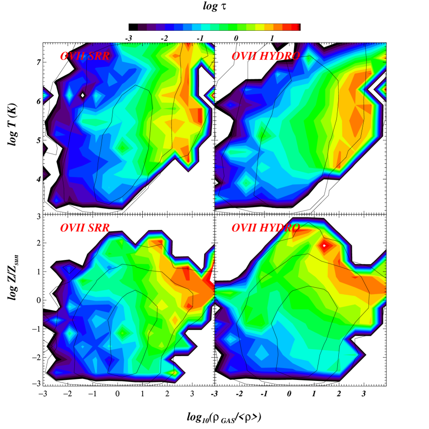
Figure 5: Filled contour plots represent the optical depth binned as a function of gas density (x-axis) and metallicity (bottom panels, y-axis) and temperature (top panels, y-axis). The results shown in the left panels have been obtained with our reconstruction method (SRR), while the right panels refer to gas in the hydro-dynamical simulation (HYDRO). Empty contour plots (black contours) represent the number density of pixels. The number density increases by an order of magnitude with each contour level.

Figure 6: Left: Probability distribution function (pdf) for the transmitted flux in OVII (filled triangles) and in OVIII (empty triangles) for the hydro-simulation. The continuous and dashed lines show the probability distribution function for the reconstructed flux in OVII and OVIII, respectively. The dotted line refers to the probability distribution function for OVII in the case in which scatter in the reconstruction method has been switched off. Right: The power spectrum of the transmitted flux in OVII and OVIII for the hydro-simulation and from our reconstruction procedure. The same symbols/line-styles are used.

The aim of this subsection is to compare the X-ray absorption features associated to the OVII and OVIII ions in the original hydro-dynamical simulation with those obtained from the full reconstruction procedure described in Section 4. In order to do that, we draw spectra from the simulation box from which we compute both the optical depth and transmitted flux due to OVII and OVIII absorbers and compare them with the same quantities obtained from the results of 30 independent reconstructions.

In Figure 5 the filled contour plots represent the optical depth in OVII binned as a function of the gas density and metallicity (bottom panels) and gas density and temperature (top panels). The left panels show the results of one of our reconstructed maps (SRR) while the results in the right panel refer to the original hydro-dynamical simulation. The empty contours (black line) represent the number density distribution of the pixels in the whole simulations (i.e. essentially the filled contours of Figure 1). We have explicitly checked that we obtain very similar results for OVIII absorbers.

This figure shows that there is a reasonable agreement between the hydro-dynamical simulation and our reconstructions method at least for the optical depth of the simulated OVII and OVIII absorbers. This agreement indicates that our reconstruction method succeeds in placing the gas responsible for absorption in OVII and OVIII in the same environments as in the original hydro-simulation, i.e. within regions of quite high metallicity, $Z>0.1\,Z\odot$, and temperature in the range $10^{5}<T(K)<10^{7.5}$.

In the left panel of Figure 6 we show the one point probability distribution function (PDF) of the transmitted flux in OVII and OVIII, while in the right panel we show the power spectrum of the transmitted flux. In both plots the triangles refer to the hydro-dynamical simulation while the continuous lines show the average over 30 independent reconstructions performed with our technique. The results, which are similar for both the OVII and OVIII absorbers, show that while the flux probability distribution functions are reproduced very well, as we expect given the constraints on the mass PDF, the power spectra of the transmitted flux show some disagreement. In the range $1<k\;(\ {\rm{\it h}\,Mpc^{-1}})\;<5$ the flux power spectrum of the hydro-dynamical simulations is about $\sim 60\%$ higher than the reconstructed one. We note that this discrepancy is somewhat larger than the corresponding one for the mass density field shown in the right panel of Figure 3. Moreover, in that case the reconstructed power at similar wavenumbers was systematically larger, not smaller, than the true one. We regard this lack of power in the transmitted flux as determined by the large amount of scatter involved in our modelling, that might reduce the spatial correlation between the absorbers on scales between 1 and 5 $\ {\rm{\it h}\,Mpc^{-1}}$. On the other hand, at wavenumbers larger than $k=0.3\;\ {\rm{\it h}\,Mpc^{-1}}$, i.e. on small scales, the power is reasonably well preserved in both the flux and the mass density field.

In addition, we show the flux probability distribution function and the flux power spectrum for a case in which any form of scatter has been switched off (i.e. instead of Montecarlo sampling the probability distribution functions as described in Section 4.3, we simply adopt the deterministic mean relations). We can see, as expected, that the flux 1-point pdf is very different especially for large absorbers. This means that the strongest absorptions in the spectra can only be reproduced by taking into account the large scatter in the temperature-density and metallicity-density relations. This confirms, at least qualitatively, the results of Chen et al. 2003 and Viel et al. 2003. Switching off the scatter also affects the predicted flux of the absorbers that systematically underestimates that measured in the hydrodynamical simulation by a factor $\sim 2.5$.

In Figure 7 we show the cumulative number of absorbers in the hydro simulations, per unit redshift range as a function of their column density (bottom axis), i.e. the number of systems with column density larger than a given value, and as a function of the corresponding equivalent width (top axis), for OVII (filled triangles) and OVIII (open triangles). The relation between the absorber equivalent width and the column density is taken from Sarazin (1989) and represents a good approximation for column densities smaller than $10^{15}\rm{cm}^{-2}$. The continuous and dashed lines represent the results obtained from our reconstruction method and refer to OVII and OVIII, respectively. The comparison with the hydro-dynamical simulation shows that our reconstruction method is capable of reproducing the correct number of systems with column density $\geq 3\times 10^{13}\rm{cm}^{-2}$. Discrepancies exist for small absorption systems that, however, could be detected neither with present nor with next generation instruments (Viel et al. 2003).

Figure 7: The cumulative column density distribution function for OVII and OVII (i.e. the number of systems per unit redshift with an equivalent width larger than a given value), as obtained from the hydro-dynamical simulations (triangles - HYDRO) and with our reconstruction method (lines - SRR). The symbols/line-styles are the same as in Figure 6. The top axis shows the corresponding column density in OVII.

Figure 8: Constrained probability of finding an absorber in the hydro-dynamical simulation map given the detection of a corresponding absorber in the reconstructed (SRR) maps. This probability has been computed via hits-and-misses statistics using 2 velocity bins of $100\ {\rm km\,s^{-1}}$ (continuous line) and of $200\ {\rm km\,s^{-1}}$ (dashed line). The dotted line refers to SRR simulations in which any form of scatter has been taken out from the modelling. Error bars represent the scatter around the mean value of the probability in each column density bin. The random coincidence level for a $\Delta v=200$ km/s is shown as the horizontal thick dot-dashed line. The thin dot-dashed line shows the relation between the column densities of the absorbers reconstructed with the technique described in Section 5, and the absorbers found in the hydro-dynamical simulation (which has to be read on the right Y-axis), for coincident systems.

As a final test, we have quantified the ability of reproducing the correct number and equivalent width of the absorption lines in simulated X-ray spectra by means of a hits-and-misses statistics. For this purpose we have only considered the spatial distribution of the OVII absorbers in the hydro-simulation and in the 30 independent reconstructions. We use only the OVII absorbers for the reason that, for a fixed column density, the corresponding equivalent width in OVII is about a factor 2 higher than the OVIII one. This means that probably OVII absorbers can be detected in slightly lower density environments than the OVIII ones.

We have drawn 1000 independent spectra in the original hydro-simulation box and along the corresponding line of sights in each of the 30 SRR reconstructions. A positive coincidence is found when an absorber in the hydro simulation is identified within a bin $\Delta v=100\ {\rm km\,s^{-1}}$ (or $\Delta v=200\ {\rm km\,s^{-1}}$) measured along the spectrum, centered on each absorber identified in the reconstructed maps. This procedure allows us to evaluate the constrained probability of finding an absorption feature in the hydro-dynamical simulation associated to a simulated (SRR) absorber in the reconstructed spectrum, binned as a function of the column density of the latter.

The results are displayed in Figure 8 where it is shown that the probability an OVII absorption line in the reconstructed spectrum associated to an absorber identified in the hydro-simulations, ranges between 0.4 and 0.6 for the smaller velocity bin and is weakly dependent on the column density. For the larger velocity bin, $\Delta v=200\ {\rm km\,s^{-1}}$, the probability is larger and ranges from 0.5 to 1 with a stronger dependence on column density. In this second case, all the SRR absorbers with column density larger than $10^{16}$ cm^-2 have a corresponding absorber in the hydro-dynamical simulations.

We note that the result is both robust, since the probability changes by a factor $\sim 1.5$, for column densities $\raise-2.0pt\hbox{\hbox to0.0pt{\hbox{$\sim$}\hss}\raise 5.0pt\hbox{$<$}\ }10^{15.3}$ cm^-2, when using two different velocity bins $\Delta v=100$ and $200\ {\rm km\,s^{-1}}$ and significant, since the error bars are small enough for the measured probability to be higher that the random coincidence level (thick dot-dashed line). In this figure we also plot the probability of finding an absorber obtained after having switched off any form of scatter in the temperature-density and metallicity density relations (dotted line). We can notice that the probability significantly decrease by a factor 1.3.

However, the fact that our method is capable of reproducing absorption features at the correct location $\geq 50\%$ of the times does not necessarily imply that the correct column density of the absorbers is reproduced too.

The thin dot-dashed in Fig. 8 shows a fit to the relation between the column density of the OVII absorbers in the reconstructions (X axis) and the average column density of the corresponding absorbers in the hydro-simulation (Y axis on the right). The correlation shows that on average the column density of the corresponding system found in the hydro-simulations is $\sim$ 20% larger that the simulated (reconstructed) one. This means that our reconstruction method tends to underestimate the actual detectability of the WHIM absorbers.

Overall our results indicate that our reconstruction method is capable of reproducing the spatial distribution and the physical properties of the gas responsible for the absorptions in OVII and OVIII and that our maps of the WHIM can be used to predict the location and detectability of these structures in the Local universe with a success rate of at least $\sim 50\%$, increasing with the column density of the absorber.

6 Temperature and metallicity maps of the local Universe

In this Section we apply our method to investigate the spatial distribution and the physical properties of the WHIM in the real universe. For this purpose we apply our reconstruction procedure described in Section 4 to the Tully catalog of nearby galaxies and produce 30 independent maps of the intergalactic gas in the local universe that account for both the stochasticity on the biasing relation and the scatter in the relations shown in Fig. 1. As we have explicitly checked, switching off the stochasticity of the bias, i.e. assuming that the bias is deterministic, does not modify our results in term of WHIM properties (WHIM properties are in very good agreement with the maps with stochasticity). This means that all the sources of scatter that we add into the model, after having produced the dark matter density field, i.e. the gas density, gas temperature, and gas-metallicity scatter, are dominant compared to the scatter induced by the stochasticity of the bias.

We will focus on the general properties of the local WHIM and on our ability to map the OVII and OVIII absorbers in the local observed universe. In addition, we will present an example of the modelling applied to the Virgo Cluster region in Section 6.1.

The three plots of Figure 9, show the predicted relation between our input galaxy luminosity field and the properties of our WHIM model, i.e. they illustrate to what extent the galaxy luminosity traces the properties of the intergalactic gas in the local universe. The results are very similar to those displayed in Figure 1, which, however, constitute an ingredient of our reconstruction scheme. The curves and the scatter are fairly similar in the two cases, showing that regions of high galactic luminosity $\delta_{\rm L}^{\rm S}\raise-2.0pt\hbox{\hbox to0.0pt{\hbox{$\sim$}\hss}\raise 5.0pt\hbox{$>$}\ }10$ are typically associated to the WHIM structures, although the scatter in the temperature and metallicity of the gas is very large. In the same Figure 9 we overplot as a dashed line the same quantities as extracted from the fiducial hydro-dynamical simulations (the 25$/h$ comoving Mpc model $768^{3}$ cells rebinned into a $256^{3}$). We note that there is in general a reasonably good agreement between the SRR method and the hydro-dynamical simulations, showing once more the goodness of our reconstruction procedure.

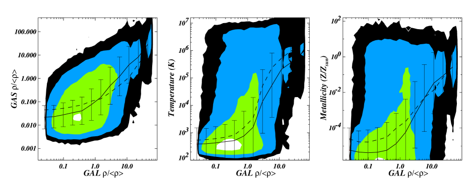
Figure 9: Left: Relation between galaxy density as derived from the galaxy catalog and the overdensity (left panel), temperature (middle) and metallicity (right) of the gas. The median values in each bin are shown as continuous lines while the error bars $1\sigma$ rms value. The filled contour plots have the same meaning as in Figure 1. The dashed line represent the same information as extracted directly from our fiducial hydro-dynamical simulations (see Section 3.)

In Figure 10 we plot the (unconstrained) probability of finding a pixel with an OVII optical depth above a given value ($\tau_{threshold}$), calculated from the set of 30 realizations of the local universe, as a function of the galaxy luminosity density in the Tully catalog. We stress that in this case we do not look for coherent systems in the simulated maps of the universe, as we did in Section 5.2, but we simply check for a pixel in the simulated maps to have an optical depth in OVII above a given threshold. Indeed, if we assume the optical depth to be small ($\tau<<1$) and constant within the system, then an approximate relation between equivalent width and optical depth is given by: $W(\ {\rm km\,s^{-1}})=\tau\,\Delta v$, where $\Delta v$ is the spatial extent of the absorber expressed in $\ {\rm km\,s^{-1}}$. In the following we will not address the distribution of equivalent widths (or column densities) in coherent systems. Rather, we keep $\Delta v$ fixed and equal to the resolution of the simulated spectra, i.e. we consider the distribution of the optical depth in each pixel. The rationale behind this statistics is to investigate the relation between WHIM and overdensity in galaxies, and to quantify how likely absorption features can be detected as a function of the density of the environment.

The left panel of Figure 10 shows the cumulative probability of a pixel with $\tau>0.1$ as a function of the galaxy luminosity density in the reconstructed maps (thick, continuous line). Pixels with $\tau>0.1$ have a probability to be detected larger than 50% in environments with $\delta>10$ and this probability becomes equal to 100% for $\delta\sim 30$. This means that in our model the very dense regions are always polluted with metals that produce OVII absorptions. However, such a small optical depth will be difficult to observe given the uncertainties in the source continuum and the low signal-to-noise of the observed spectra, unless they are organized in a spatially coherent system along the line of sight. If we ask for stronger absorptions to take place one can see that pixels with an OVII optical depth above 0.5 (2.5) are associated with galaxy overdensities of $\delta>16$ ($\delta>48$) with a probability larger than 50% (35%). In the right panel of Figure 10 we plot the probability map of an optical depth larger than 0.1 in a slice of thickness $\sim 0.3\ {\rm{\it h}^{-1}Mpc}$ containing the Virgo cluster. The region around Virgo is visible as a prominent clump at $(SGX,SGY)=(-3,12)$, characterized by the presence (probability = 1) of OVII absorbers. The thin lines plotted in the left panel of Figure 10 shows the cumulative probability of a pixel with $\tau>\tau_{threshold}$ in a spherical region of radius $2.5\ {\rm{\it h}^{-1}Mpc}$ centered around the Virgo Cluster. In this case the probabilities are larger than in the whole simulated local universe (up to a factor 2 for $\tau_{threshold}=0.5$) because the coherent structure of the Virgo cluster is quite well reproduced by our simulated maps.

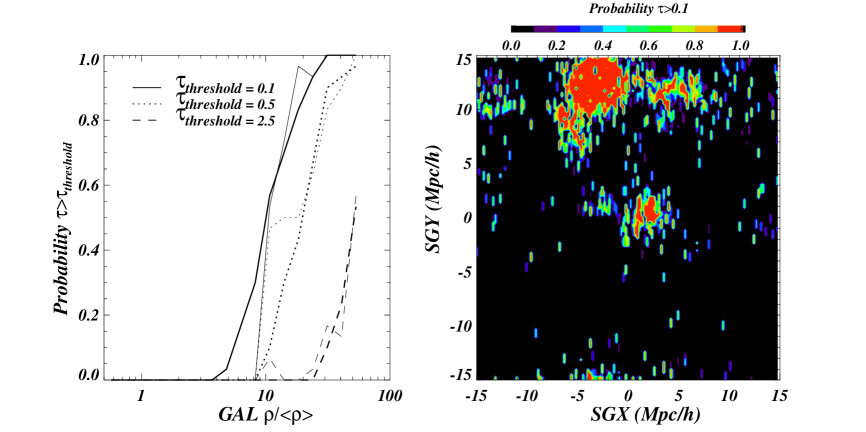
Figure 10: Left: Probability of finding an optical depth in OVII larger than a given value, $\tau_{threshold}$, in the local universe as a function of the density in galaxies. The thin lines indicate the same probability as extracted in a smaller spherical region of radius $\sim 2.5\ {\rm{\it h}^{-1}Mpc}$ around the center of the Virgo Cluster. Right: Contour plots of the probability of detecting an absorption with a $\tau>0.1$ in a slice of $\sim 0.3\ {\rm{\it h}^{-1}Mpc}$ centered around the Virgo Cluster.

6.1 Warm Hot Intergalactic Medium in the Virgo Cluster: a semi-analytical study

In the previous section we have shown that a semi-quantitative study of the WHIM detectability in the local universe can be done with our technique.

Motivated by the fact that WHIM structures could be detected with a significant probability around the Virgo cluster, we study in a more quantitative way, the properties of the WHIM and its detectability in this region using our semi-analytical technique. In addition, we investigate the robustness of our predictions by exploring the effect of galactic winds and of the scatter in the relations shown in Fig. 1 implemented into the model.

In the left panel of Figure 11 we show the mass density field, obtained from the galaxy density field, smoothed with a Gaussian filter of radius $95\ {\rm km\,s^{-1}}$, assuming the mean biasing relation (i.e. stochasticity off). As we have just pointed out, the Virgo Cluster region could be very promising for detecting the WHIM component since the typical overdensity reconstructed with our technique could be larger than $100$ in a region of about $(2{\rm{Mpc}}/h)^{3}$ around the cluster centre, while it drops significantly at larger distances.

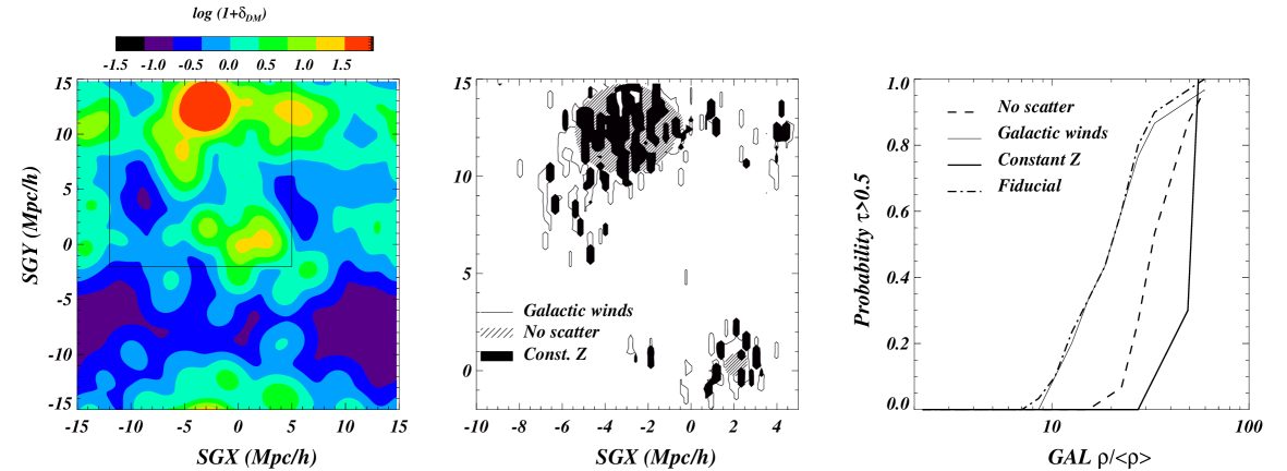
Figure 11: Left: Slice of $\sim 0.3$ Mpc$/h$ around the Virgo Cluster representing the smoothed dark matter density field derived from the galaxy catalog of Tully (1988). The box indicates the region around the Virgo cluster which is considered in the other two panels. Center: Map of the regions with probability larger than 0.5 of an absorber with an optical depth in OVII higher than 0.5 in the area around the Virgo Cluster. Iso-probability contours traced with a continuous line refer to the case of strong galactic winds, with the metallicity-density relation right panel of Fig. 2. The dashed regions refer to a model in which any form of scatter in the gas density, temperature and metallicity vs. dark matter density relations is switched off. The filled contours refer to a model in which the metallicity has been set to a constant value of 0.3 Z_⊙, which is the mean metallicity of the simulated box. Right: Probability of having an absorption feature with optical depth in OVII higher than 0.5 as a function of galactic overdensities in the regions around the Virgo Cluster. The result of our fiducial model is represented by the dot-dashed line. The thin continuous line represents the case of a the model with galactic winds. The thick continuous line and the dashed line show the models with constant metallicity and no scatter, respectively.

In the middle panel of Figure 11 we zoom on a smaller region around the Virgo cluster and we check how different implementations of our semi-analytical modelling will affect the WHIM detectability. All contours represented here enclose regions with probability $>0.5$ of finding an OVII absorber (pixel) with optical depth $\tau>0.5$. In particular, since in Section 6, we have already explored the probability of detecting WHIM features with our fiducial model (25$/h$ Mpc $768^{3}$ mesh rebinned into a $256^{3}$ mesh – see Section 3) based on the relations shown in Figure 1, we want to explore the effect of modifying those relations on the predicted WHIM property in the regions around Virgo. We focus on the effect of galactic winds, of the scatter in the different relations and on the shape of the metallicity-density relation. The iso-probability contours enclosed by a continuous line refer to a model in which the effect of strong galactic winds is taken into account, i.e. when we use the metallicity-density relation shown in the left panel of Figure2, rather than that of Figure 1 (while we keep the other relations to be those of Figure 1).

The shaded areas refer instead to a model in which any form of scatter in the different relations of Figure 1 is switched off. Finally, the filled contours refer to a model in which the metallicity is assumed to be constant to a value of 0.3 $Z_{\odot}$, which is the mean metallicity of our fiducial simulation. One can see that galactic winds, which are effective in polluting the intergalactic medium, produce a non negligible detectability of WHIM structures at smaller overdensities than in the other two cases. The fiducial model, i.e. that for which the relations of Figure 1 hold, produces results very close to the galactic winds case. In the model without scatter, instead, the distribution of the OVII absorbers closely traces that of the mass, as expected. In this case the regions containing OVII absorbers wit $\tau>0.5$ are smaller than in the galactic wind case, meaning that the intrinsic scatter in the different relations is effective in enhancing the WHIM detectability as found by Chen et al. (2003) and Viel et al. (2003). The model with a constant metallicity set to a value of 0.3 $Z_{\odot}$ tends to produce detectable regions only in very dense environments. This means that a significant fraction of the absorption can come from regions at higher metallicities than these (see Figures 1 and 2).

In order to be more quantitative we plot in the right panel of Figure 11 the cumulative probability of a pixel with an OVII optical depth $>0.5$, as a function of the galactic overdensity of the Tully catalog for the various models explored. The probability associated to the model with galactic winds (thin continuous line) is significantly larger than for the two other models, even at moderate overdensities of 10. We note however that there is very little difference between this line and the dot-dashed one, which refers to our fiducial simulation, i.e. the one in which we have implemented the relations shown in Figure 1. It seems that winds are effective in transporting metals into the low density regions but they produce little effects on the denser structures in which WHIM absorption takes place. This means that our prediction for the WHIM distribution are robust since they are weakly affected by the presence of strong galactic winds. This issue will be investigated in more detail in a future work. In the rather unphysical case of pure deterministic relations between the IGM properties, i.e. the case of no scatter (dashed line), the probability decreases by a factor of 2 in the range of overdensities 20-40. The lack of any correlation between density and metallicity (thick continuous line) has an even more dramatic effect since in this case one could hope to detect OVII absorptions features only in the few higher density regions (although this of course depends on the value chosen for the constant metallicity level).

We stress here that the modelling presented in this paper offers not only predictions for observers on where to look at in order to detect WHIM structures but allows to put constraints on the state of the IGM even if OVII and OVIII lines are not detected along a particular line-of-sight.

7 Discussion and conclusions

Motivated by the recent interest in the warm-hot phase of the intergalactic medium and by the present difficulty of its detection, we have developed a semi-analytic model capable of predicting the spatial distribution of the WHIM in the local supercluster, its physical properties and the probability of detecting it through absorption lines in the X-ray spectra of bright background extragalactic sources.

Unlike the models previously proposed by Kravtsov, Klypin & Hoffman (2002) and by Yoshikawa et al. (2004) our technique does not require to perform a full hydro-dynamical simulation. Instead, since it uses the already existing outputs of numerical simulations, it requires much less CPU time to model the WHIM in the local universe from the observed high resolution map of galaxy light density. As a consequence we are able to i) trace the distribution of mass and gas with a resolution of $\sim 1\ {\rm{\it h}^{-1}Mpc}$ (Gaussian) and ii) perform several independent realizations to account for the model uncertainties, through which we can quantify the probability of detecting an absorption feature at a given redshift in an X-ray spectrum drawn along an arbitrary direction in the sky.

The most serious drawback of our technique is the lack of self-consistency in the reconstruction procedure which results in a lack of spatial coherence on sub-Mpc scales that prevents us from reconstructing the properties of the IGM in the local universe on a point-by-point basis. However, as we have explicitly checked through extensive numerical tests, our model correctly predicts the spatial location and the physical conditions of the WHIM, that typically resides in regions of enhanced densities. We have focused on the OVII and OVIII ions that are responsible for the strongest WHIM absorption features in the X-ray spectra and have shown that our model correctly reproduces the statistical properties of the WHIM absorbers. In particular, we are able to reproduce the correct number of absorption systems per unit redshift as a function of the column density, especially for absorbers with large equivalent width. Moreover, we are able to predict the correct spatial location of the OVII absorbers 40-70% of the times, significantly above the random level, and up to 100% for systems with column density of $\sim 10^{16}{\rm cm}^{-2}$, although we somewhat underestimate their actual equivalent width. Finally, our semi-analytic technique is capable of reproducing the global physical properties of the IGM, quantified in terms of gas density, temperature and metallicity vs. galaxy light density relations.

It is worth pointing out that several alternative routes to our reconstruction procedure are also possible. A very interesting one, proposed by the anonymous referee, consists of mapping galaxy light density to OVII and OVIII density without any reference to the matter density field. The idea is to determine the distribution of OVII and OVIII in the hydrodynamical simulation and use their 1-point PDF in the inversion procedure described in Section 4.1 to map galaxy light to OVII and OVIII density in the local universe, hence avoiding mapping mass to intergalactic gas (Section 4.3) which represents the main source of scatter in our method. Unfortunately, as we have verified, the mean OVII and OVIII vs galaxy density relation flattens out and becomes non monotonic when the density increases. As a result, it is not possible to trace OVII and OVIII in regions of enhanced densities where the stronger absorbers typically resides unless the inversion method of Section 4.1 could be suitably modified.

Encouraged by our ability of mapping the distributions of OVII and OVIII in our local universe, we have focused on the region around the Virgo Cluster. We found a large ($>0.5$) probability of an OVII absorber with opacity ($\tau>0.5$) in each resolution element contained in a quasi-spherical region of radius $2.5\ {\rm{\it h}^{-1}Mpc}$ centered on the Virgo Cluster that therefore represents the most promising site for detecting WHIM in the local universe (hence confirming, at least qualitatively, the results of Kravtsov, Klypin & Hoffman (2002)). This prediction is robust, since the size of this region and the probability detection level do not change significantly when one allows for uncertainties in modeling the IGM properties. In addition we have studied the effect of strong galactic winds that are effective in polluting low density regions, but seems not to appreciably affect regions of enhanced density where OVII and OVIII absorbers are preferentially located. We have found that using deterministic relations to describe the IGM properties can be quite dangerous, as it would result in a significant underestimate of the occurrences of OVII and OVIII absorbers in low density regions (an effect that becomes even more dramatic when assuming an IGM with constant metallicity).

This semi-analytic model is therefore able to map the probability of detecting absorbers associated to the highly ionized ions in the WHIM, and to predict the equivalent width of the corresponding absorption features in X-ray spectra. This is of considerable observational interest since it allows us to quantify the probability of observing absorption features in the spectra of all bright X-ray sources, produced by the WHIM in the Local Supercluster. Moreover, since our method somewhat under predicts the column density of the absorber, we will also be able to provide a lower limit to the significance of detecting such features with a specified instrument. It is worth stressing that this method offers the possibility to put constraints on the physical properties of the IGM (metallicity, temperature, ionization state) even in the presence of non detections of OVII and OVIII absorbers along a particular line-of-sight and not only when these WHIM absorption features are detected.

Obviously, our model is also able predict the emission lines produced by the very ions responsible for the X-ray absorption features very much like in the recent study of Yoshikawa et al. (2004), although on a much more local basis.

Our model predictions can be cross-correlated with existing X-ray spectra to increase the significance of marginal detections of absorption lines.

It is worth stressing that while our modeling is performed in real space, absorption features are observed in redshift space. Redshift space distortions can be easily accounted for in our modeling by displacing the line-of-sight position of the X-ray absorbers according to some of the available model velocity field, like the non-parametric one of Branchini et al. (1999). These corrections are expected to be quite minor since the cosmic flow in the local supercluster is notoriously cold (Klypin et al. 2003).

Our model is currently limited to a very local volume of the universe. This is the consequence of having required a very dense sampling in tracing the galaxy light. In fact, our current implementation of the light to mass tracing technique requires at least one object per resolution element, a requirement that sets the maximum size of the explored volume. More sophisticated techniques, like the one recently proposed by Szapudy & Pan (2004), can be successfully implemented in case of much sparser sampling and thus can be used to extend our WHIM predictions beyond the boundaries of the local supercluster.

References

- [] Bennett C. L., et al., 2003, AIs, 148, 1
- [] Branchini, E.; Teodoro, L.; Frenk, C. S.; Schmoldt, I.; Efstathiou, G.; White, S. D. M.; Saunders, W.; Sutherland, W.; Rowan-Robinson, M.; Keeble, O.; Tadros, H.; Maddox, S.; Oliver, S., 2000, MNRAS, 308, 1.
- [] Branchini et al. 2004, in preparation
- [] Boldt R., 1987, Phys. Rep., 146, 215
- [] Cen R., Ostriker J.P., 1999a, ApJ, 514, 1
- [] Cen R., Ostriker J.P., 1999b, ApJ, 519, L109
- [] Cen R., Nagamine K., Ostriker J.P., 2004, ApJ, astro-ph/0407143
- [] Cen R., Miralda-Escudé J., Ostriker J.P., Rauch M., 1994, ApJ, 437, L83
- [] Cen R., Kang H., Ostriker J.P., Ryu D., 1995, ApJ, 451, 436
- [] Cen R., Tripp T.M., Ostriker J.P., Jenkins E. B., 2001, ApJ, 559L, 5
- [] Cen R., Ostriker J.P., Prochaska J.X., Wolfe A.M., 2003, ApJ, 598, 741
- [] Chen X., Weinberg D.H., Katz N., Davé R., 2003, ApJ, 594, 42
- [] Davé R., Hernquist L., Katz N., Weinberg D.H. , 1999, ApJ, 511, 521
- [] Davé R., Cen R., Ostriker J.P., Bryan G.L., Hernquist L., Katz N., Weinberg D.H., Norman M.L., O’Shea B., 2001, ApJ, 552, 473
- [1] Dekel A., Lahav O. 1999, ApJ, 520, 24
- [] Fabian A.C., Barcons X., 1992, ARA&A, 30, 429
- [] Ferland G.J., Korista K.T., Verner D.A., Ferguson J.W., Kingdon J.B., Verner E.M., 1998, PASP, 110, 761
- [] Fisher, J.R., Tully, R.B. 1981, ApJS, 47, 139
- [] Fukugita M., Hogan, C. J., Peebles P. J. E., 1998, ApJ, 503, 518
- [] Furlanetto S.R., Schaye J., Springel V., Hernquist L., 2004, ApJ, 606, 221
- [] Hellsten U., Gnedin N.Y., Miralda-Escudé J., ApJ, 1998, 509, 56
- [] Kaastra J.S. et al., 2003, A&A, 397, 445
- [] Klypin A., Hoffman Y., Kravtsov A.V., Gottlober S. 2003, ApJ, 596, 19
- [] Kravtsov A.V., Klypin A., Hoffman Y., 2002, ApJ, 571, 563
- [] Nicastro F. et al., 2003, Nature, 6924, 719
- [] Nicastro F. et al., 2004, astro-ph/0412378
- [] Ostriker J. P., Cen R., 1996, ApJ, 464, 270
- [2] Peebles J., 1989, ApJ, 344, L53
- [] Perna R., Loeb A., 1998, ApJ, 503, 135
- [] Rauch M., 1998, ARA&A, 36, 267
- [] Sarazin C.L., 1989, ApJ, 345, 12
- [] Savage B.D., 2003, ApJS, 146, 245
- [3] Shaya E., Peebles J., Tully B., 1995, ApJ, 415, 15
- [] Shull J.M., Roberts D., Giroux M.L., Penton S.V., Fardal M.A., 1999, AJ, 118, 1450
- [4] Sigad Y., Branchini E., Dekel A., 2000 ApJ, 540, 62
- [] Tripp T.M., Savage B.D., Jenkins E.B., 2000, ApJ, 534, L1
- [] Szapudi, I., Pan, J. 2004, ApJ, 602, 26
- [5] Tully B., 1988 “The Nearby Galaxy Catalog”, Cambridge University Press
- [] Viel M., Branchini E., Cen R., Matarrese S., Mazzotta P., Ostriker J. P., 2002, MNRAS, 341, 792
- [] Zappacosta L., Mannucci F., Maiolino R., Gilli R., Ferrara A., Finoguenov A., Nagar N.M., Axon D.J., 2002, A&A, 394, 7
- [] Yoshida N., Stoher F., Springel V., White S.D.M, 2002, 335, 762
- [] Yoshikawa K. et al., 2004, astro-ph/0408140