VLBI observations of weak sources using fast frequency switching

We have developed a new phase referencing technique for high frequency VLBI observations. In conventional phase referencing, one interleaves short scans on a nearby phase calibrator between the target source observations. In fast frequency switching described here, one observes the target source continuously while switching rapidly between the target frequency and a lower reference frequency. We demonstrate that the technique allows phase calibration almost reaching the thermal noise limit and present the first detection of the AGN in the FR I radio galaxy NGC 4261 at 86 GHz. Although point-like, this is the weakest source ever detected with VLBI at this frequency.

1 Introduction

The regions where jets from active galactic nuclei (AGN) are launched and collimated are difficult to observe with VLBI because they lie very close to the black hole and most bright objects are very distant. Thus, there are still very few observational constraints on jet formation. Only in the closest AGN can the highest resolution observations resolve several tens of Schwarzschild radii ($R_{\rm s}$), comparable to the scale of $10\,R_{\rm s}$ to $1000\,R_{\rm s}$ where jet formation is expected to take place (e.g., Koide et al. 2000, Appl & Camenzind 1993).

One of the best targets for resolving details in the jet is NGC 4261 (3C 270). It is an elliptical low-luminosity FR I radio galaxy hosting a $4.9\times 10^{8}\,M_{\odot}$ black hole (Ferrarese et al. 1996) which powers a double-sided radio jet (Jones & Wehrle 1997; Jones et al. 2000, 2001). Given the distance to NGC 4261 of 28.2 Mpc ($H_{0}={\rm 75\,km\,s^{-1}\,Mpc^{-1}}$) and its black hole mass, 86 GHz VLBI observations are expected to resolve $200\,R_{\rm s}$. This measurement would be, after diameter measurements of Sgr A* ($24\,R_{\rm s}$, Bower et al. 2004, $17\,R_{\rm s}$, Krichbaum et al. 1998) and M 87 ($32\,R_{\rm s}$, Junor et al. 1999, $46\,R_{\rm s}$, Ly et al. 2004) the third-highest resolution image ever achieved in terms of Schwarzschild radii. Furthermore, the high inclination of the jets makes NGC 4261 a good candidate to look for a core-shift with frequency. Core-shift measurements are of considerable astrophysical interest. They can help to discriminate between the conically-expanding jet model (Blandford & Königl 1979) and advection-dominated accretion flows (ADAFs, e.g., Narayan et al. 1998) in low-luminosity AGN, to find the true location of the AGN, to determine the jet magnetic field strength and to test for potential foreground absorbers (Lobanov 1998). Although NGC 4261 therefore is an interesting source to study the jet formation process, it is unfortunately not possible to directly observe NGC 4261 with 86 GHz VLBI, because it is too weak. This paper demonstrates a new calibration method that makes such an observation possible.

High frequency observations involve a number of serious problems: the sources are usually weak because the emissivity of optically thin synchrotron sources drops as $\nu^{-0.7}$, the aperture efficiencies of most of the radio telescopes drop to 15 % or less because their surface accuracies were specified for cm-wavelength operation, the receiver performances become disproportionately worse because of higher amplifier noise, the atmospheric contribution to the system temperatures increases towards higher frequency, and the atmospheric coherence that limits the integration time decreases as $1/\nu$.

However, the integration times could be prolonged if the atmospheric phase fluctuations could be calibrated. This can be done using self-calibration, or if the source is too weak, then using phase referencing (e.g., Shapiro et al. 1979; Marcaide & Shapiro 1984; Alef 1988). Both are established calibration techniques and phase referencing can be used to lower detection thresholds to the sub-mJy level and can accurately determine source positions. In phase referencing, a strong calibrator source is observed frequently (every few minutes, depending on observing frequency) to calibrate the visibility phases of the target source integrations, i.e., the telescopes cycle between the target source and the phase calibrator source. In millimetre VLBI the technique is not commonly used because of the need for a suitable, strong phase calibrator in the vicinity of the target source and from a combination of short atmospheric coherence time and relatively long telescope slewing times. However, a successful proof of concept exists for 86 GHz VLBI observations (Porcas & Rioja 2002).

In this paper, we describe a novel way of calibrating visibility phases to overcome these limitations, using interleaved observations at a low and a high frequency.

2 Principle of phase correction

2.1 Self-calibration

The phase of the complex visibility function which an interferometer measures is altered by instrumental drifts, antenna and source position errors, and path length changes in the earth’s atmosphere. These errors can be accounted for using self-calibration, which is similar to adaptive optics in optical astronomy. Starting with a point source model in the field centre, and refining the model iteratively, antenna-based correction phases are derived that make the visibility phases compliant with the model. Similar to adaptive optics, where a sufficiently bright guide star is required to detect the shape of the wavefront, self-calibration requires a minimum signal-to-noise ratio (SNR) on each baseline. Visibilities with an SNR of less than about five within the atmospheric coherence time are commonly regarded as non-detections.

2.2 Scaling and interpolation

One can self-calibrate the visibility phases at one frequency and use the solutions to calibrate visibilities at another frequency after multiplying the phases by the frequency ratio, $r$. This works since the main source of phase noise in VLBI observations at frequencies higher than about 5 GHz is turbulence in the troposphere causing refractive inhomogeneities which are non-dispersive. One requires that the lag between the two measurements does not exceed half the atmospheric coherence time (Fig. 1). Instead of using a phase-referencing calibrator source, the source is phase-referenced to itself at a lower frequency.

This is possible with the Very Long Baseline Array (VLBA, Napier et al. 1994) because frequency changes need only a few seconds, in which the subreflector is moved from one feed horn to the other, and because the local oscillator phase returns to its original setting after frequency switching. After multiplying the phase solutions by the frequency ratio and applying them to the target-frequency phases, there remains a constant phase offset, $\Delta\Phi$, between the signal paths at the two frequencies, which must be calibrated. This can be monitored with frequent observations of achromatic, strong calibrators, and must be subtracted from the high-frequency visibility phase.

The observed visibility phases using this calibration scheme can be described as

$$\begin{split}\phi_{\rm r}^{\rm obs}(t_{1})=\phi_{\rm r}^{\rm tru}(t_{1})+\phi_{\rm r}^{\rm ins}(t_{1})&+\phi_{\rm r}^{\rm pos}(t_{1})+\phi_{\rm r}^{\rm ant}(t_{1})\\ &+\phi_{\rm r}^{\rm tro}(t_{1})+\phi_{\rm r}^{\rm ion}(t_{1})\\ \phi_{\rm t}^{\rm obs}(t_{2})=\phi_{\rm t}^{\rm tru}(t_{2})+\phi_{\rm t}^{\rm ins}(t_{2})&+\phi_{\rm t}^{\rm pos}(t_{2})+\phi_{\rm t}^{\rm ant}(t_{2})\\ &+\phi_{\rm t}^{\rm tro}(t_{2})+\phi_{\rm t}^{\rm ion}(t_{2})\\ \phi_{\rm r}^{\rm obs}(t_{3})=\phi_{\rm r}^{\rm tru}(t_{3})+\phi_{\rm r}^{\rm ins}(t_{3})&+\phi_{\rm r}^{\rm pos}(t_{3})+\phi_{\rm r}^{\rm ant}(t_{3})\\ &+\phi_{\rm r}^{\rm tro}(t_{3})+\phi_{\rm r}^{\rm ion}(t_{3}).\\ \end{split}$$ (1)

Here, $\phi^{\rm tru}$ indicates true visibility phases of the source, $\phi^{\rm ins}$ is the residual instrumental phase error, $\phi^{\rm pos}$ and $\phi^{\rm ant}$ are geometric errors arising from source and antenna position errors, and $\phi^{\rm tro}$ and $\phi^{\rm ion}$ are tropospheric and ionospheric phase noise contributions. The subscript indices r and t indicate quantities that belong to the reference frequency, $\nu_{\rm r}$, and the target frequency, $\nu_{\rm t}$, respectively.

Self-calibration at the reference frequency is used to obtain a source model and hence to obtain $\phi_{\rm r}^{\rm tru}(t_{1})$ and $\phi_{\rm r}^{\rm tru}(t_{3})$. Self-calibration of the visibilities at the reference frequency after subtracting this model yields $\phi_{\rm r}^{\rm cor}$, the sum of $\phi_{\rm r}^{\rm ins}$, $\phi_{\rm r}^{\rm pos}$, $\phi_{\rm r}^{\rm ant}$, $\phi_{\rm r}^{\rm tro}$ and $\phi_{\rm r}^{\rm ion}$. This sum is linearly interpolated to the times where the target frequency was observed, and is scaled by the frequency ratio, $r$:

$$r\tilde{\phi}_{\rm r}^{\rm cor}=r(\tilde{\phi}_{\rm r}^{\rm ins}+\tilde{\phi}_{\rm r}^{\rm pos}+\tilde{\phi}_{\rm r}^{\rm ant}+\tilde{\phi}_{\rm r}^{\rm tro}+\tilde{\phi}_{\rm r}^{\rm ion}),$$ (2)

where a tilde denotes quantities linearly interpolated to time $t_{2}$. The difference between the target frequency visibility phase and the interpolated and scaled reference frequency correction phase at time $t_{2}$ is then

$$\begin{split}\phi_{\rm t}^{\rm obs}-r\tilde{\phi}_{\rm r}^{\rm cor}=\phi_{\rm t}^{\rm tru}&+(\phi_{\rm t}^{\rm ins}-r\tilde{\phi}_{\rm r}^{\rm ins})+(\phi_{\rm t}^{\rm pos}-r\tilde{\phi}_{\rm r}^{\rm pos})\\ &+(\phi_{\rm t}^{\rm ant}-r\tilde{\phi}_{\rm r}^{\rm ant})+(\phi_{\rm t}^{\rm tro}-r\tilde{\phi}_{\rm r}^{\rm tro})\\ &+(\phi_{\rm t}^{\rm ion}-r\tilde{\phi}_{\rm r}^{\rm ion}).\end{split}$$ (3)

The instrumental phase offset, $\Delta\Phi=(\phi_{\rm t}^{\rm ins}-r\tilde{\phi}_{\rm r}^{\rm ins})$, is constant with time and can be determined from calibrator observations, and so it is known and can be removed. The antenna position error, like all geometric errors, scales with frequency and hence $(\phi_{\rm t}^{\rm ant}-r\tilde{\phi}_{\rm r}^{\rm ant})=0$. A frequency-dependent core shift, however, as predicted by conical jet models (e.g., Lobanov 1998), modulates $(\phi_{\rm t}^{\rm pos}-r\tilde{\phi}_{\rm r}^{\rm pos})$ on each baseline with a sinusoid. The period of the sinusoid is $23^{\rm h}56^{\rm m}$, its amplitude depends on the magnitude of the shift and its phase depends on the direction of the shift relative to the baseline direction. It is zero only in the absence of a core shift, and therefore provides useful structural information. The tropospheric phase errors also scale with frequency, and hence $(\phi_{\rm t}^{\rm tro}-r\tilde{\phi}_{\rm r}^{\rm tro})=0$. The ionospheric phase errors do not scale linearly with frequency and so cannot be removed using this technique, requiring that they be measured separately. We assume for the moment that this has been done, but see the next section for the impact of ionospheric effects on the data presented here. The remaining terms describe the difference between the target frequency phase and the scaled and interpolated reference frequency phase corrections as the target frequency visibility phase plus the position offset:

$$\phi_{\rm t}^{\rm obs}-r\tilde{\phi}_{\rm r}^{\rm cor}=\phi_{\rm t}^{\rm tru}+(\phi_{\rm t}^{\rm pos}-r\tilde{\phi}_{\rm r}^{\rm pos}).$$ (4)

Thus, the true high-frequency visibilities are phase-referenced to the source’s low-frequency visibilities, and so the technique can prolong coherence and can measure the position shift of cores in AGN with frequency.

2.3 Ionospheric path length changes

For illustration, we assumed in the previous section that the ionospheric effects were calibrated. Ionospheric path length changes can probably be determined using interspersed, wide-band scans at a low frequency, e.g., in the 1.4 GHz band, where the effect is strong. We had not appreciated before observing that the ionosphere would still be significant at 15 GHz and had not planned 1.4 GHz scans to measure ionosphere. Hence, the high-frequency visibilities from the observations presented here contained unmodelled ionospheric path length changes which limited the coherence to half an hour in the worst case. To remove the remaining long-term phase drifts and remaining phase offsets required one extra step of self-calibration. This step of self-calibration loses source position information, which prevented a core-shift measurement from being made. Still the extension from the 30 s atmospheric coherence time to a coherent integration time of 30 min yielded a large sensitivity improvement and allows weaker sources to be detected.

A similar observing strategy has been developed by Kassim et al. (1993) for the VLA, who used scaled phase solutions from 330 MHz to calibrate simultaneously observed 74 MHz data. In this case, the dominant source of phase errors was ionospheric path length changes. Using their new calibration technique, they were able to increase the coherent integration time from $<$ 1 min to $>$ 10 min and to make 74 MHz images of several radio sources. Fast frequency switching is also being considered as a standard calibration mode for the Atacama Large Millimeter Array (ALMA) in the future (D’Addario 2003).

Figure 1: Demonstration of the scalability of phase solutions. 43 GHz fringe-fitted phase solutions (solid lines) on 3C 273 compared to 15 GHz fringe-fitted phase solutions multiplied by the frequency ratio (dashed lines) from the VLBA antennas at Hancock (upper panel) and Kitt Peak (lower panel) to the reference VLBA antenna at Los Alamos. The phases follow each other very well.

3 Observations

Source	Duration	Freq.	3C 279	5	43
	(min)	pair	3C 273	5	43
(1)	(2)	(3)	3C 273	5	1
OJ 287	10	15-86	NGC 4261	25	15-43
OJ 287	10	15-43	3C 273	5	15-43
NGC 4261	25	15-43	3C 273	5	15-86
3C 273	5	15-43	NGC 4261	25	15-86
NGC 4261	25	15-86	3C 279	5	15-43
3C 273	5	15-86	3C 279	5	15-86
3C 273	5	15-43
			3C 273	10	15-43
OJ 287	5	15a			15-
OJ 287	5	43a	NGC 4261	25	15-43
OJ 287	5	86a	3C 273	5	15-43
			3C 273	5	15-86
NGC 4261	25	15-43	NGC 4261	25	15-86
3C 279	5	15-43	3C 279	5	15-86
3C 279	5	15-86	3C 279	5	15-43
3C 273	5	15-86
3C 273	5	15-43	3C 279	5	15a
NGC 4261	25	15-43	3C 279	5	43a
3C 273	5	15-43	3C 279	5	86a
3C 273	5	15-86
NGC 4261	25	15-86	3C 273	5	15-43
3C 279	5	15-86	3C 273	5	15-86
3C 279	5	15-43	NGC 4261	25	15-86
			3C 273	5	15-86
3C 273	10	15-43	3C 273	5	15-43
			NGC 4261	25	15-43
NGC 4261	25	15-43	3C 279	5	15-43
3C 273	5	15-43	3C 279	5	15-86
3C 273	5	15-86	3C 273	5	15-43
NGC 4261	25	15-86
3C 279	5	15-86	3C 345	5	15a
			3C 345	5	43a
3C 279	5	15a	3C 345	5	86a
3C 279	5	43a
3C 279	5	86a	3C 345	10	15-43
			3C 345	10	15-86

Table 1: Summary of observations May 5, 2003. The sources observed are in column (1), the scan duration is in column (2) and the frequency pairs in GHz are in column (3). An $a$ indicates fringe finder scans during which no frequency switching was done.

We observed NGC 4261 on May 5, 2003 with the ten VLBA stations and we interleaved observations of 3C 273 and 3C 279 to calibrate the inter-frequency offset and to test the technique on strong sources. Dynamic scheduling allowed us to observe during a period of good to excellent weather at most stations, using 256 Mbps to record a bandwidth of 64 MHz with 2-bit sampling. We recorded LCP only, the data were divided into 8 IFs with 8 MHz bandwidth, each of which were subdivided into 64 spectral channels 125 kHz wide. The correlator integration time was one second to allow monitoring of the phases with high time resolution. All antennas performed well, except for Fort Davis, where a receiver problem caused complete loss of 43 GHz data. A summary of this observing run is given in Table 1.

In this paper, two integrations at $\nu_{\rm r}$ and $\nu_{\rm t}$ are called a “cycle”, each integration of which is called a “half-cycle”, and a sequence of cycles on the same source is called a “scan”. Long (several minutes), continuous integrations on a single source at one frequency, e.g. fringe-finder observations, are also called “scans”.

Several considerations influenced the experiment design.

3.1 Frequency choice

The target frequency should be an integer multiple of the reference frequency to avoid having to unwrap phase wraps. For example, if the frequency ratio, $r$, is the non-integer value of 2.5, and the reference frequency phase wraps from $359^{\circ}$ to $0^{\circ}$, then the scaled target frequency phase will jump from $897.5^{\circ}$ ($=177.5^{\circ}$) to $0^{\circ}$, introducing a phase jump of $177.5^{\circ}$ into the calibration phase for a $1^{\circ}$ phase change at $\nu_{\rm r}$. In contrast, choosing $r=2.0$, when the reference frequency phase wraps from $359^{\circ}$ to $0^{\circ}$, the scaled target frequency phase changes from $718^{\circ}$ ($=358^{\circ}$) to $0^{\circ}$, corresponding to a change of $2^{\circ}$ for a $1^{\circ}$ phase change at $\nu_{\rm r}$. Hence, for integer values of $r$, phase wraps at the reference frequency introduce integer multiples of $360^{\circ}$ at the target frequency and so have no effect.

We chose a reference frequency of 14.375 GHz since the third and sixth harmonics at 43.125 GHz and 86.25 GHz lie within the VLBA receiver bands. For convenience, we will refer to these frequencies as “15 GHz”, “43 GHz” and “86 GHz”, respectively. These frequencies should then be shifted slightly to end in .49 MHz or .99 MHz to allow correct operation of the VLBA pulse calibration detection system, and the final two digits should not change during the experiment as a change causes a time-consuming reconfiguration of the formatter. Thus, optimal frequencies are 14.37499 GHz, 43.12499 GHz and 86.24999 GHz.

3.2 Integration times

We chose a cycle time of 50 s, of which 22 s were spent at the reference frequency of 15 GHz and the remaining 28 s were spent at the target frequency, either 43 GHz or 86 GHz. An average time of 7 s per half-cycle was lost in moving the subreflector between the feed horns, resulting in net integration times of 15 s at $\nu_{\rm r}$ and 21 s at $\nu_{\rm t}$. The integration times are a compromise, depending on source brightness, antenna sensitivity and expected weather conditions. This setup yielded a $5\,\sigma$ detection limit of 89 mJy in 15 s at 15 GHz for the VLBA on a single baseline.

3.3 Calibrator scans

Calibrators must be observed frequently to monitor the phase offset $\Delta\Phi=\phi_{\rm t}^{\rm ins}-r\tilde{\phi}_{\rm r}^{\rm ins}$ between the two frequencies. A constraint which is important for core-shift measurements is that the calibrators must be achromatic, i.e., they must not have their own frequency-dependent core shifts. In the case of the observations presented here, uncalibrated ionospheric errors prevented such a measurement of $\Delta\Phi$. We used self-calibration with a long solution interval to calibrate the residual phase errors, and did not require measurement of the instrumental phase offset on calibrators.

As the core-shift information is not generally available, the best strategy is to observe at least two calibrators to test for a possible core shift in the calibrators. We included adjacent scans on two different calibrators to measure $\Delta\Phi$ before and after target source observations. Five of the calibrator scans were twice as long to provide more time for tests with strong signals.

4 Data reduction

4.1 Standard steps

Data reduction was carried out in AIPS. A calibration table entry was generated every 4.8 s to provide high temporal resolution. The amplitudes were calibrated using $T_{\rm sys}$ and gain measurements provided by automatic noise-adding radiometry, and amplitude corrections for errors in the sampler thresholds were performed using autocorrelation data. Phase corrections for parallactic angles were applied (this step is not strictly required for the method to work) and a simple bandpass correction was derived at each frequency from one of the fringe finder scans.

The VLBA’s pulse calibration system did not deliver data to calibrate the phase offsets between the IFs because the frequencies were changed too quickly. The pulse calibration system has a default integration time of 10 s, plus one second for readout. If any part of that integration time is during a part of the scan that is flagged by the online system, then the integration is not accepted. Thus, one loses the first two integrations because the online system conservatively flags 10 s to 11 s after a frequency change, and there is an overlap between the flagged time and the second integration. During the whole experiment, only $\sim 10$ useful pulse-cal measurements were recorded per station at 15 GHz (half-cycle time 22 s), and $\sim 100$ at 43 GHz (half-cycle time 28 s), compared to the number of half-cycles at these frequencies of $\sim 630$ and $\sim 230$, respectively. We therefore used fringe-fitting on the same fringe finder scans as were used for bandpass calibration to correct for instrumental delays and inter-IF phase offsets. These offsets were found to be stable over the experiment.

4.2 Ionospheric correction

Although the frequencies used in the project are quite high, ionospheric effects can not be neglected and will prevent a successful phase transfer if uncorrected. A typical ionospheric delay at a frequency of $\nu_{1}=100$ MHz is 0.1 $\mu$s (10 turns of phase), but can be up to $10\,\mu{\rm s}$. The exact number strongly depends on the time of day, time of year and time in the solar cycle. The delay scales with frequency as $\nu^{-2}$, and so for a delay at 100 MHz of 0.1 $\mu$s, the ionospheric delays at 14.37499 GHz, 43.12499 GHz and 86.24999 GHz are 4.84 ps, 0.54 ps and 0.13 ps, respectively, corresponding to $25^{\circ}$, $8.4^{\circ}$ and $4.0^{\circ}$ of phase. The linear phase versus frequency scaling law used by fast frequency switching cannot correct phase changes that are induced by the ionosphere. Ionospheric phase changes have much longer time-scales than tropospheric changes, and they can be calibrated before fringe-fitting when the electron content of the ionosphere along the line of sight is known. The AIPS task TECOR can use maps of ionospheric total electron content (TEC) derived from GPS data to calculate phase and delay corrections. Unfortunately, the error in these maps can be quite high, up to 20 % when the TEC is as high as a few tens of TEC units (1 TEC unit equals $10^{16}\,{\rm electrons\,m^{-2}}$), and up to 50 % or higher when the TEC is of the order of a few TEC units. We have used the TEC maps produced by the Center for Orbit Determination in Europe (CODE) to calibrate the effects of the ionosphere. We found that these maps yielded slightly better results than those from the Jet Propulsion Laboratory (JPL), i.e., the residual phase errors after scaling were smaller. We do not know whether this finding is coincidental or whether the CODE maps generally give better results.

4.3 Effect of frequency changes on the phases

Amplitudes needed 2 s to 3 s longer to reach their final values during a frequency change than did the phases. Thus, the visibility phases are not very sensitive to even large errors in subreflector rotational position. The repeatability of the phases from cycle to cycle shows that positioning the subreflector along the optical axis is repeatable to $<5^{\circ}$ of phase at 15 GHz, which is much less than other sources of phase error in fast frequency switching. Six to seven seconds at the beginning of each half-cycle, when the subreflector was moved between feed horns, needed to be flagged.

4.4 Phase solution and phase scaling

We derived phase solutions at 15 GHz using fringe-fitting, which is equivalent to self-calibration except that it also derives delay solutions. Its sensitivity therefore is not as good as self-cal, which performs a phase search only and is preferred. However, fringe-fitting yielded good results and a high detection rate in our experiment.

We fringe-fitted the 15 GHz data using the AIPS task FRING, with an SNR threshold of 5 and delay and rate search windows of 20 ns and 50 mHz, respectively. As NGC 4261 has an extended, double-sided jet structure at 15 GHz, we made a 15 GHz image which we used as a source model in a second run of FRING, so that the phase solutions did not contain structural phase contributions. The solution interval was set to 1 min, yielding one phase, delay and rate solution per half cycle. The detection rate was $\sim 90\,\%$. The 15 GHz solution (SN) table was written to a text file with TBOUT to do the phase scaling outside AIPS. We have written a Python program (FFSTG, the Fast Frequency Switching Table Generator) that processes an SN table in the following way.

First, a series of timestamps is generated from each pair of consecutive entries in the input table such that they coincide with the $\nu_{\rm t}$ half-cycles. Second, from each pair of consecutive $\nu_{\rm r}$ phase solutions, a solution is interpolated for the new timestamps consisting of a phase, a phase rate derived from the $\nu_{\rm r}$ phase solutions and the time interval between the $\nu_{\rm r}$ scans, and an interpolated delay. Both the phase rate and the delay do not need to be scaled by $r$ because the rate is stored in a frequency-independent format (in units of ${\rm s\,s^{-1}}$) and the delay is non-dispersive. Third, the interpolated phase solution is scaled by the frequency ratio, $r$, yielding $\nu_{\rm t}$ phase solutions for the times at which the source was observed at $\nu_{\rm t}$.

We did not use the phase rates derived by fringe-fitting because each of those was derived from one half-cycle of 22 s length, whereas the phase rates interpolated from two consecutive half-cycles as described above used two half-cycles separated by 50 s and therefore have much better SNR. This requires the phase to change by less than $180^{\circ}$ in 50 s, which was the case during our experiment due to sufficiently short half-cycles. A further advantage of deriving phase rates from pairs of phase solutions is that each $\nu_{\rm r}$ phase solution is used both in the determination of the phase rate to the preceding and the succeeding $\nu_{\rm r}$ solution, causing a smoothing of the phases with time and reducing the effect of outliers. Finally, the interpolated phase, phase rate and delay solutions are stored in an output table together with the $\nu_{\rm t}$ frequency ID. FFSTG provides an interface to Gnuplot to plot and inspect the input and output phases. One can select regions of interest and check the results of the scaling.

The table was imported to AIPS using TBIN and was used to update the most recent calibration table at the target frequency.

5 Results

5.1 43 GHz

(a) NGC 4261 raw 43 GHz visibility phases on baselines to Los Alamos with only delay calibration applied.

(b) NGC 4261 calibrated 43 GHz visibility phases on baselines to Los Alamos. Calibration used scaled-up phase solutions from fringe-fitting with a clean component model at 15 GHz, but no ionospheric correction has been applied.

(c) NGC 4261 calibrated 43 GHz visibility phases on baselines to Los Alamos. Calibration used ionospheric corrections and scaled-up phase solutions from fringe-fitting with a clean component model at 15 GHz. The residual phase rates are much lower than in Fig. 2(b).

Figure 2: Raw and calibrated visibility phases on baselines to Los Alamos. Each data point is an average over a half-cycle.

Figure 3: Enlarged sections of Fig. 2(a) (left panel) and 2(c) (right panel).

NGC 4261 was detected on most baselines at all times after scaling the 15 GHz solutions to 43 GHz. Here, the term “detected” means that by inspecting the phase time series by eye one could see that the phase was not random. The correlated flux densities range from 30 mJy on baselines of 800 M$\lambda$ to 160 mJy on baselines of 30 M$\lambda$. The 43 GHz half-cycle average visibilities on baselines to LA are shown in Figs. 2 and 3. The short-term fluctuations introduced by the troposphere are almost perfectly calibrated, but residual phase drifts remain on longer time-scales, especially at the beginning (before and during sunset) and at the end of the experiment, when the source elevation was lower.

5.1.1 Structure functions

Structure functions of the 43 GHz visibility phases from a 25 min scan on NGC 4261 are shown in Fig. 4 showing the data at each stage of calibration. Phase wraps have been removed, allowing phase differences exceeding $360^{\circ}$.

The structure functions constructed from the calibrated phase time-series show a residual phase noise on the shortest time-scales (50 s) of $50^{\circ}$ early in the observations and of $33^{\circ}$ in the middle of the experiment (taking the median of the phase noise of all baselines). The phase noise increases toward longer time-scales, probably due to errors in the ionospheric models. Evidence for the long-term phase noise being dominated by ionosphere is as follows.

First, applying an ionospheric TEC correction significantly improved the coherence, as one can see by comparing Figs. 2(b) and 2(c). Second, the residual phase errors decreased in the middle of the experiment, when the average elevation of the source was $58^{\circ}$. During the first scan at 01:00 UT, the average source elevation at all antennas was $32^{\circ}$, hence the line of sight through the ionosphere was 63 % longer, amplifying errors in the ionospheric model. Also, the experiment began briefly before sunset at the stations in the south-west US. This is a time of rapidly changing ionospheric TEC causing unstable phases early in the experiment on baselines to the south-western stations.

We fringe-fitted the 43 GHz data calibrated with fast frequency switching with a solution interval of 30 min to remove the residual long-term phase drifts. The structure functions after applying this correction are shown as dotted lines in Fig. 4; the long-term phase noise is reduced as expected, and the phase noise on 50 s time scale is slightly lower, with a median of $44^{\circ}$ during the beginning and $31^{\circ}$ in the middle of the experiment.

Figure 4: Structure functions of the phase time series from 25 min of observation of NGC 4261 at 43 GHz. Solid lines show raw data observed in the middle of the experiment with delay calibration only. The data were averaged in frequency and over each half-cycle. Dashed lines show the same data calibrated with scaled-up phase solutions from fringe-fitting at 15 GHz, and dotted lines show the same data after fringe-fitting with a 30 min solution interval. Phase wraps have been removed. The horizontal dashed lines indicate the theoretical phase noise. The median residual phase noise of calibrated data with residual phase rates is $33^{\circ}$ on a 50 s time-scale, and without residual phase rates is $31^{\circ}$.

5.1.2 Expected phase noise

The expected phase noise in the visibilities calibrated with fast frequency switching consists of five parts: (1) thermal phase noise at the reference frequency scaled by the frequency ratio, (2) thermal phase noise at the target frequency, (3) tropospheric phase changes during the two integrations, (4) ionospheric scintillations and (5) errors in the source model at the reference frequency. Estimates of these contributions are as follows.

The $1\,\sigma$ thermal noise on a baseline is given by

$$\Delta S=\frac{1}{\eta_{\rm s}}\times\frac{SEFD}{\sqrt{2\times\Delta\nu\times\tau}}$$ (5)

(Walker 1995), where $\eta_{\rm s}$ is an efficiency factor (0.69 for the VLBA with 2-bit sampling as we used), $SEFD$ is the antenna’s system equivalent flux density in Jy, $\Delta\nu$ is the bandwidth in Hz and $\tau$ the integration time in seconds.

The typical measured $SEFD$ for the VLBA antennas was 550 Jy at 15 GHz, 1436 Jy at 43 GHz and 5170 Jy at 86 GHz (at 43 GHz and 86 GHz, these numbers are fairly variable between antennas). In our observations, $\tau$ was 15 s at 15 GHz and 21 s at 43 GHz and 86 GHz, and $\Delta\nu$ was 64 MHz. One therefore expects thermal noise levels of 18.2 mJy, 40.1 mJy and 145 mJy at 15 GHz, 43 GHz and 86 GHz, respectively. At 15 GHz, NGC 4261 has a correlated flux density, $S$, between $60\,{\rm mJy}$ and $300\,{\rm mJy}$, depending on baseline length, so we adopt either $80\,{\rm mJy}$, representative of long baselines, or $200\,{\rm mJy}$, representative of short baselines (the results of which we give in brackets).

(1)

On a single baseline, the expected SNR of a detection at 15 GHz is $S/\Delta S=80\,{\rm mJy}/18.2\,{\rm mJy}=4.61$ (11.0) when averaging over the band. Fringe-fitting, however, uses all baselines to one particular antenna to derive a phase correction, and so the SNR is increased by $\sqrt{N}$, where $N$ is the number of baselines. $N\approx 8$, so the SNR of a detection at 15 GHz increases to 12.4 (31.1). We have converted the SNR into a visibility phase rms using the following approach. Let us assume that the phase of the true visibility is 0. The probability distribution of the measured visibility phase as a function of SNR, $p(\phi)$, is given in Eq. 6.63b in Thompson et al. (2001). The square of the phase rms derived from that probability is:

$$\sigma^{2}=\frac{\int\phi^{2}p(\phi)d\phi}{\int p(\phi)d\phi}$$ (6)

We have evaluated the integral numerically and find a phase rms of $4.61^{\circ}$ ($1.84^{\circ}$). This phase noise is scaled by the frequency ratio to $13.8^{\circ}$ ($5.53^{\circ}$) at 43 GHz and $27.6^{\circ}$ ($11.1^{\circ}$) at 86 GHz.

(2)

Assuming that NGC 4261 has a compact flux density of 100 mJy at both 43 GHz and 86 GHz, the thermal noise contributions according to Eq. 6 are $26.3^{\circ}$ and $76.0^{\circ}$, respectively. Adding those in quadrature to the scaled-up thermal rms phase noise from 15 GHz yields $29.7^{\circ}$ ($26.9^{\circ}$) at 43 GHz and $80.9^{\circ}$ ($76.8^{\circ}$) at 86 GHz.

(3)

We estimated the tropospheric phase noise within the switching cycle time using structure functions of 3C 273. On 3C 273, the thermal noise contributions at 15 GHz and 43 GHz are $0.04^{\circ}$ and $0.4^{\circ}$, respectively, so that the visibility phases are essentially free of thermal noise and any phase changes during and between the half-cycles are due to changes in the troposphere. We found the median rms phase noise on a 50 s time-scale after fringe-fitting with a 30 min solution interval to remove the residual long-term phase drift to be $13.3^{\circ}$ at 43 GHz, or $26.6^{\circ}$ at 86 GHz.

The amplitudes of (4) (ionospheric scinitillations) were found to be less than three radians at 378 MHz on time-scales up to 40 s by Yeh & Liu (1982). When scaled to 15 GHz, they contribute only $0.1^{\circ}$ on time-scales of 40 s, and even less at the higher frequencies, so their contribution remains miniscule and is no longer considered. The contribution of (5) (errors in the source model) is also not significant. First, these errors do not contribute a noise-like component but rather long-term phase errors similar to errors in the TEC model. Second, phase corrections at 15 GHz to account for the source structure were at most $50^{\circ}$ in 6 h, or $3.5^{\circ}$ in 25 min, and only on the longest baselines. This means that introducing a source model at all required changes of order a few degrees per 30 min. Errors in the model, however, are expected to be much smaller because the sampling of the $(u,v)$ plane at 15 GHz was excellent. They should barely exceed $1^{\circ}$ at 15 GHz, or $3^{\circ}$ at 43 GHz. This is much less than all other source of phase noise, and can therefore be neglected.

Adding the first three non-negligible noise components in quadrature yields $32.6^{\circ}$ ($30.0^{\circ}$) at 43 GHz and is in excellent agreement with the measured rms phase noise of $31^{\circ}$.

5.1.3 Coherence

   

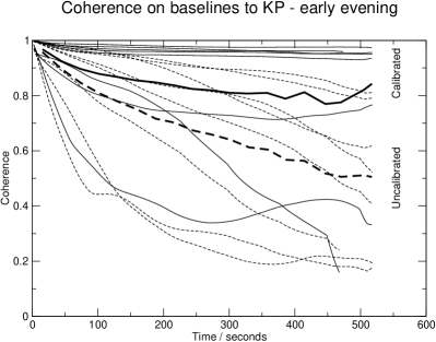
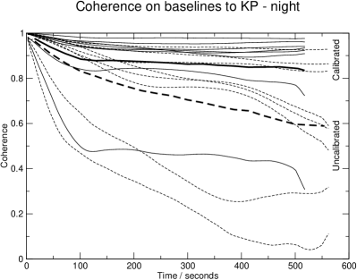
Figure 5: Coherence diagrams showing the improvement achieved at 43 GHz using fast frequency switching. The vector sum over progressively longer time intervals has been computed on all baselines and has been normalized by the scalar sum of the vectors, after setting the phases to zero. Bold lines show the average over all baselines in bins of 28 s, i.e., the length of one half-cycle. The coherence was analysed using visibilities on baselines to Kitt Peak, which had moderate to good (but not excellent) weather conditions, and hence is representative for the array performance during the observing run. Shown are 3C 273 data observed in the beginning (centred on 03:20 UT, left panel) and the middle (centred on 06:50 UT, right panel) of the experiment at 43 GHz with interleaved 15 GHz observations for calibration. 43 GHz data from 10 min scans with (solid lines) and without (dashed lines) phase calibration from 15 GHz have been averaged in frequency. As 3C 273 is strong, the data are essentially free of thermal noise and show the coherence improvement with fast frequency switching.

Another way of illustrating the performance of the corrections is with coherence diagrams (Fig. 5). For the plots shown, 3C 273 43 GHz data from all baselines to KP have been used. All data were calibrated using fast frequency switching (no subsequent fringe-fitting), and were averaged over the band and in time to obtain one visibility per baseline and half-cycle. The vector average of these visibilities has been computed over progressively longer time intervals and normalized by the scalar average.

The left panels show data from a 25 min scan centred on 03:20 UT and the right panels show data from a 25 min scan centred on 06:50 UT. Bold lines show the average over all baselines. The coherence achieved in the middle of the experiment with fast frequency switching is a little better than that achieved during the beginning of the observations.

5.1.4 Stability of the phase offset

After correction of the ionopheric phase errors, the visibility phases on the LA-PT baseline were stable to $<$1 rad over 10 h (Fig. 2(c)). This indicates that the instrumental phase offset, $\Delta\Phi$, was also stable within the same limits, and it appears to be sufficient to determine $\Delta\Phi$ a few times throughout the experiment.

5.1.5 Imaging

Before making an image from the 43 GHz visibilities calibrated with fast frequency switching, the residual phase offsets and phase rates were removed using fringe-fitting with a solution interval of 30 min so that one solution per scan was obtained. The resulting dirty image (Fig. 6) has a peak flux density of $79\,{\rm mJy\,beam^{-1}}$ and an rms noise of $4.4\,{\rm mJy\,beam^{-1}}$, yielding a dynamic range of 18:1. After several cycles of phase self-calibration with a solution interval of 30 s and one cycle of amplitude self-calibration with a solution interval of 12 h, the peak flux density was $95\,{\rm mJy\,beam^{-1}}$ and the rms noise was $0.78\,{\rm mJy\,beam^{-1}}$, so the dynamic range improved to 122:1 (Fig. 7). The theoretical rms noise at 43 GHz was expected to be $0.46\,{\rm mJy\,beam^{-1}}$. Unfortunately, the ionospheric phase errors and the need to fringe-fit to calibrate them did not allow a core shift measurement to be made.

Our final image has a synthesized beam size of $0.42\,{\rm mas}\times 0.25\,{\rm mas}$, corresponding to a linear resolution of $720\,R_{\rm s}$. This is about 50 % larger than achieved by Jones et al. (2000) with conventional, non-phase-referencing 43 GHz VLBA observations. The difference in resolution is due to two factors. First, we made only few detections on baselines to Mauna Kea. This is because Mauna Kea was observing at predominantly low elevations, hence suffering more from ionospheric phase errors. Second, we used natural weighting to increase sensitivity to extended structures, whereas Jones et al. (2000) used uniform weighting for increased resolution.

Notwithstanding these differences, our 43 GHz image is very similar to that published as Fig. 5 in Jones et al. (2000). Both observations show a dominant core and a jet extending 1.4 mas to the west, with indications of emission at 2 mas west of the core. Both images indicate the presence of a counterjet extending up to 1 mas east of the core. However, Jones et al. (2000) find a peak flux density of 141 mJy beam^-1, whereas we find a peak flux density of 95 mJy beam^-1. The observations were separated by 5.7 yr, and source variability may have caused some (or all) of the difference. Furthermore, changing tropospheric opacity during either observation may have affected the peak flux density. In our image, the eastern jet looks smooth, whereas it shows components in the observation of Jones et al. (2000). This probably arises from the different weighting schemes and image fidelity limits, rather than from a real change of jet character.

Figure 6: Naturally weighted, full-resolution dirty image of NGC 4261 at 43 GHz, calibrated with scaled-up phase solutions from 15 GHz. Fringe-fitting has been used to solve for one residual phase and rate solution per 25 min scan before exporting the data to Difmap. No further self-calibration has been applied. The image noise is 4.4 mJy beam^-1 and the dynamic range is 18:1. The synthesized beam size is $0.38\,{\rm mas}\times 0.18\,{\rm mas}$. The bar in the upper left corner shows the size of the minor axis.

Figure 7: Data and imaging parameters as in Fig. 6, but several cycles of phase self-calibration with a solution interval of 30 s and one cycle of amplitude self-calibration with a solution interval of 12 h have been applied. The final image was cleaned and has an rms noise of 0.78 mJy beam^-1 and a dynamic range of 122:1. The synthesized beam size is $0.42\,{\rm mas}\times 0.25\,{\rm mas}$. The bar in the upper left corner shows the size of the minor axis.

5.2 86 GHz

Figure 8: 86 GHz visibility phases. Top: NGC 4261 raw 86 GHz visibility phases on baselines among Fort Davis, Kitt Peak, Los Alamos, Owens Valley and Pie Town with only delay calibration applied. Bottom: 86 GHz visibility phases on baselines among Fort Davis, Kitt Peak, Los Alamos, Owens Valley and Pie Town. Calibration has been done with scaled-up phase solutions from fringe-fitting at 15 GHz using a clean component model. Good detections were made during almost every 25 min scan observed at night between 2:00 UT and 7:00 UT, when the source elevation was high and ionospheric effects lower.

Figure 9: Structure functions of a 25 min scan at 86 GHz, showing the same stages of calibration as in Fig. 4. Note that the expected noise level, indicated by the horizontal dashed lines, is a guideline only. It depends on the correlated source flux density which varies with baseline length and orientation (see Section 5.2).

Figure 10: The coherence improvement at 86 GHz with fast frequency switching on baselines to KP, obtained in the same way as for Fig. 5. However, we did not observe any calibrator long enough to generate coherence plots, so the diagram was constructed from NGC 4261 data. The coherence therefore is significantly lowered by thermal noise.

Figure 11: Naturally weighted, full-resolution dirty image of NGC 4261 at 86 GHz, calibrated with scaled-up phase solutions from 15 GHz. Fringe-fitting has been used to solve for one residual phase and rate solution per 25 min scan before exporting the data to Difmap. No further self-calibration and no deconvolution has been applied. The image noise is 8.4 mJy beam^-1 and the dynamic range is 7:1. The synthesized beam has a diameter of $0.35\,{\rm mas}\times 0.54\,{\rm mas}$ in P.A. $11^{\circ}$ and corresponds to a linear resolution of 0.048 pc or $1000\,R_{\rm s}$. The bar in the upper left corner shows the size of the minor axis.

Figure 12: Naturally weighted, full-resolution clean image of NGC 4261 at 86 GHz using the same data and calibration as in Fig. 11. No further self-calibration has been applied. The image noise is 7.5 mJy beam^-1 and the dynamic range is 8:1. The synthesized beam has a diameter of $0.28\,{\rm mas}\times 0.52\,{\rm mas}$ in P.A. $19^{\circ}$ and corresponds to a linear resolution of 0.038 pc or $800\,R_{\rm s}$.

Following the same data reduction path as for the 43 GHz data, we obtained good detections of NGC 4261 at 86 GHz on baselines among the four stations FD, KP, LA, and PT and only weak detections on baselines to NL, OV and MK. Again, a “detection” means that in a plot of visibility phase with time as in Fig. 8, one can see that the phases cluster and are not random.

Uncorrected and corrected visibility phases are plotted in Fig. 8. The improvement in coherence is clearly visible as a pronounced clustering of points in the lower panel, compared to quasi-random phases in the upper panel. Structure functions and coherence plots from a 25 min scan of NGC 4261 are shown in Figs. 9 and 10. The coherence improvement is especially pronounced on the FD-LA baseline (upper left panel in Fig. 9), whereas the improvement on the PT-LA and OV-LA baselines is small. The coherence plot in Fig. 10 shows that the coherence on baselines to KP increased from 35 % to almost 60 % on time-scales of 20 min.

A dirty image is shown in Fig. 11 and a cleaned image in Fig. 12. The peak flux density is 59.3 mJy. This is the first detection of NGC 4261 with VLBI at 86 GHz. It is also probably the weakest continuum object ever detected with VLBI at this frequency. The next brightest detection of which we are aware is 85 mJy in the 86 GHz image of $1308+328$ by Porcas & Rioja (2002), using conventional phase referencing to a calibrator $14.3^{\prime}$ away. With only delay calibration applied, the median rms phase noise of the best 25 min scan is $104^{\circ}$, after applying the scaled 15 GHz phase solutions is $70^{\circ}$ and after fringe-fitting with a 30 min solution interval is $80^{\circ}$. The increase in rms phase noise after removal of phase rates is unexpected and has an unknown cause.

The expected thermal phase noise is the quadrature sum of the scaled-up 15 GHz noise and the 86 GHz noise, the former of which we estimated to be $27.6^{\circ}$ on long and $11.1^{\circ}$ on short baselines, and the latter, assuming a correlated flux density of 100 mJy and using Eq. 6, is $76.0^{\circ}$. The quadrature sum is $80.9^{\circ}$ on long and $76.8^{\circ}$ on short baselines, and adding the tropospheric phase errors of $26.6^{\circ}$ is $85.1^{\circ}$ and $81.3^{\circ}$, in agreement with the measured noise levels.

Note that these numbers provide a guideline only. The largest contribution to the expected 86 GHz noise is the $76.0^{\circ}$ from thermal noise in the 86 GHz receivers. This number depends on the source flux density which is a strong function of baseline length and orientation. For example, the average visibility amplitude on the relatively short FD-LA baseline was 180 mJy at 4:30 UT (not 100 mJy as adopted above), reducing the 86 GHz thermal noise to $55.2^{\circ}$. The expected total phase noise, indicated by the dashed horizontal line in the upper left panel in Fig. 9, then drops to $62.3^{\circ}$.

The rms noise in the final 86 GHz image is $7.4\,{\rm mJy\,beam^{-1}}$, compared to an expected thermal noise of $3.7\,{\rm mJy\,beam^{-1}}$. The dynamic range in the image is 7:1.

5.3 Discussion of the 86 GHz image

The final 86 GHz image of NGC 4261 in Fig. 12 has a synthesized beam size of $0.28\,{\rm mas}\times 0.52\,{\rm mas}$ in P.A. $19^{\circ}$, which is about 12 % larger than the clean beam of the 43 GHz image. This is mostly due to the lack of detections on long baselines and the phase noise arising from low elevations at Mauna Kea (see Section 5.1.5) was larger by a factor of two at 86 GHz than at 43 GHz due to the higher frequency. The VLBA station at Hancock was being commissioned at 86 GHz and the station at Brewester was not equipped at 86 GHz; both would have contributed long baselines at this frequency. Also, the complete loss of 43 GHz data at Fort Davis resulted in poorer sampling of short $(u,v)$ spacings at 43 GHz but not at 86 GHz, so there is an emphasis on long baselines at 43 GHz and on short baselines at 86 GHz. The resolution at 86 GHz corresponds to 0.038 pc, or $800\,R_{\rm s}$, at the distance of NGC 4261.

The image displays a point source only; further self-calibration of the data did not reliably converge on any extended structure. The point source is probably the brightest component seen in the 43 GHz image, which probably corresponds to the jet base. Our observations therefore did not allow us to resolve the jet collimation region. However, we are confident that the suggested improvements to the observing strategy to calibrate ionospheric phase errors can significantly improve the detection rates on long baselines and hence increase the resolution.

6 Benefits of fast frequency switching

The primary use of fast frequency switching is to detect sources that are too weak for self-calibration at the target frequency within the atmospheric coherence time, but can be reliably detected at a lower frequency. The $5\,\sigma$ detection limit of the VLBA at 43 GHz within 120 s, with 64 MHz bandwidth and 2-bit sampling, and neglecting coherence loss due to tropospheric phase changes, is 84.0 mJy (i.e., a thermal noise level of 16.8 mJy on a single baseline). The $1\,\sigma$ noise level using fast frequency switching with half-cycle times of 22 s at 15 GHz and 28 s at 43 GHz (yielding net integration times of 15 s and 21 s, respectively), after one cycle is 67.7 mJy, of which 40.1 mJy is thermal noise in the raw 43 GHz visibility, 54.6 mJy is thermal noise in the phase solutions after scaling from 15 GHz, and neglecting noise due to tropospheric phase changes. The $1\,\sigma$ noise level after 120 s of fast frequency switching (i.e., 2.4 cycles) is 43.7 mJy. The noise level of fast frequency switching reaches that of a conventional 120 s integration at 43 GHz of 16.8 mJy after 812 s (13.5 min). Any longer integration with fast frequency switching then yields detection thresholds that are out of reach with conventional methods.

Furthermore, the proposed application of fast frequency switching to detect core shifts in AGN can supplement jet physics with observational constraints which are otherwise difficult to obtain.

Fast frequency switching is limited by the source strength at the reference frequency, and 100 mJy at 15 GHz is, from our experience, a reasonable minimum required for a successful observation. Many sources exist that meet this criterion. The 130 sources in the 2 cm VLBI observations by Kellermann et al. (1998), for example, have peak flux densities of 100 mJy beam^-1 or more; all of them can be observed at 86 GHz using fast frequency switching.

Another estimate of the number of new sources made accessible to 86 GHz VLBI by fast frequency switching can be made by means of the $\log N-\log S$ relation. Let us assume that the sources observable with conventional 86 GHz VLBI are distributed homogeneously in an Euclidean universe, so that lowering the detection limit does not yield the detection of a new population. The number of sources above a given flux-density limit, $S$, then increases as $S^{-1.5}$. We further make the conservative assumption that these sources have $\alpha=0$ between 15 GHz and 86 GHz, because they are compact.

The current $5\,\sigma$ detection limit of the VLBA at 86 GHz is 605 mJy (five times the thermal noise of a 30 s integration with 64 MHz bandwidth and 2-bit sampling on a single baseline). In fringe-fitting, all $N$ antennas are used to derive a phase solution, so the noise level is reduced by $\sqrt{N}$, and with $N=8$, the $5\,\sigma$ detection limit is 214 mJy. Fast frequency switching allows one to observe any compact source with $S_{\rm 86\,GHz}\geq 100\,{\rm mJy}$, a factor of 2.14 fainter than with conventional methods, and one expects 3.1 times as many sources brighter than 100 mJy than there are brighter than 214 mJy, following the $\log N-\log S$ relation. A little less conservative estimate would be to allow for spectral indices as steep as $\alpha=-0.3$, so that sources with $S_{\rm 15\,GHz}=100\,{\rm mJy}$ have $S_{\rm 86\,GHz}>60\,{\rm mJy}$. The number of observable sources would then increase by a factor of 6.7 times the number accessible to conventional techniques.

The absolute number of presently observable sources is much more difficult to determine due to selection effects in the various radio source catalogues. However, we can make a simple estimate using the recent 86 GHz VLBI survey by Lobanov et al. (2002). They aimed at observing more than 100 sources selected from the literature that had an expected compact flux density of $S_{\rm 86\,GHz}>300\,{\rm mJy}$. Applying the fast frequency switching sensitivity estimates then yields between 520 and 1100 sources observable with the VLBA at 86 GHz.

7 Summary

1. Fast frequency switching can be used to calibrate tropospheric phase fluctuations if the switching cycle time is shorter than the atmospheric coherence time. The accuracy is limited by tropospheric phase changes between and during the reference frequency integrations.

2. Insufficient knowledge about the ionosphere’s total electron content (TEC) has prevented calibration of the inter-band phase offset and hence it was not possible to make a pure phase-referenced image without using self-calibration. This also prevented the detection of a core shift. Current global TEC models derived from GPS data have errors that are too large to sufficiently calibrate the ionospheric component of the phase changes. A possible solution is to insert frequent (every 10 min) scans in the 1.4 GHz band with widely separated IF frequencies to derive the ionospheric delay on the line of sight to the target source.

3. On the most stable baseline between LA and PT, the instrumental phase offset was stable to $<$1 rad over 10 h. It therefore seems to be sufficient to determine the offset a few times throughout the experiment.

4. Truly simultaneous observations at two bands would reduce the residual phase errors even further because tropospheric phase changes within the switching cycle time would be entirely removed.

5. At 86 GHz, NGC 4261 was detected as a point source with 59.3 mJy beam^-1 flux density and so is the weakest source ever detected with VLBI at that frequency. Our observation at 43 GHz yielded a resolution corresponding to $720\,R_{\rm s}$ and hence ranks among the highest resolutions achieved in any AGN in terms of Schwarzschild radii.