First microlensing candidate towards M31 from the Nainital Microlensing Survey

We report our first microlensing candidate NMS-E1 towards M31 from the data accumulated during the four years of Nainital Microlensing Survey. Cousin $R$ and $I$ band observations of $\sim 13^{{}^{\prime}}\times 13^{{}^{\prime}}$ field in the direction of M31 have been carried out since 1998 and data is analysed using the pixel technique proposed by the AGAPE collaboration. NMS-E1 lies in the disk of M31 at $\alpha=0^{h}43^{m}33^{s}.3$ and $\delta=+41^{\circ}06^{{}^{\prime}}44^{{}^{\prime\prime}}$, about 15.5 arcmin to the South-East direction of the center of M31. The degenerate Paczyński fit gives a half intensity duration of $\sim$ 59 days. The photometric analysis of the candidate shows that it reached $R\sim 20.1$ mag at the time of maximum brightness and the colour of the source star was estimated to be $(R-I)_{0}\sim 1.1$ mag. The microlensing candidate is blended by red variable stars; consequently the light curves do not strictly follow the characteristic Paczyński shape and achromatic nature. However its long period monitoring and similar behaviour in $R$ and $I$ bands supports its microlensing nature.

1 Introduction

Recent years have seen rapid advances in our understanding of the nature of dark matter in the Galaxy. Much of this progress has come from the studies of gravitational microlensing, a phenomenon of temporary amplification of the flux of a background star when a foreground MACHO passes close to our line of sight to this background star. In the last decade, several collaborations have focused their attention on Galactic bulge and Magellanic Clouds following the suggestion of Paczyński (1986) and reported more than one thousand microlensing events after monitoring millions of star in these directions (e.g. Alcock et al. 1993 for MACHO, Udalski et al. 1993 for OGLE and Aubourg et al. 1993 for EROS collaborations). These groups have ruled out most of the dark matter in the form of sub-stellar objects and estimated that only up to 20% of the halo could be made up of MACHOs in the mass range of $0.15M_{\odot}$ to $0.9M_{\odot}$ (Alcock et al. 2000., Lasserre et al. 2000).

Although the conventional microlens monitoring is successful towards the Galactic bulge and Magellanic Clouds, it is fundamentally limited to only nearby regions where there are large number of resolved stars. In regions like M31, which is at $\sim$ 780 kpc (Stanek & Garnovich 1998, Joshi et al. 2003), microlens monitoring is a cumbersome process due to the large background of unresolved stars of M31 where the typical stellar density is as high as few hundred stars per arcsec². To deal with this problem, Baillon et al. (1993) proposed to monitor pixels of the CCD rather than the stars themselves. Any variation in the flux of stars due to microlensing would be determined in the corresponding variation in the pixel of the CCD. Therefore, by monitoring a pixel for a long time, one could detect a microlensing event. The pixel technique, which relies on the shape analysis of the light curve to detect microlensing events, is implemented by the AGAPE (Ansari et al. 1997) and POINT-AGAPE collaborations (Paulin-Henriksson et al. 2002) and have reported more than 10 possible microlensing events towards M31 (Calchi Novati et al. 2002, 2003, Paulin-Henriksson et al. 2002, 2003). A similar approach but based on the image subtraction technique was proposed by Crotts (1992) and Tomaney & Crotts (1996) that has been further improved by Alard & Lupton (1998) and Alard (2000) by optimal image subtraction using a space-varying kernel. The technique is widely used to detect different kinds of variable sources (cf. Bonanos et al. 2003; Taylor 2004). Recently the MEGA collaboration reported 14 microlensing candidates in their survey towards M31 using the image subtraction technique (de Jong et al. 2003). Two of them (ML-7 and ML-11) had already been reported by POINT-AGAPE in their survey using the pixel technique (PA-99-N2 and PA-00-S4 respectively). Both the groups give similar results although derived by two different techniques.

Although pixel lensing technique allows us to detect microlensing events where the standard technique of microlens detection is not applicable, it is limited to only bright stars that are either giants and super-giants or stars that are amplified enough to become detectable above the noise level of background flux. Since the search for gravitational microlensing events requires monitoring of millions of stars over a few years to yield a significant number of detections as well as to test their uniqueness, we started multi-band observations of M31 in the autumn of 1998 under a program Nainital Microlensing Survey at the ARIES, Nainital, India in collaboration with the AGAPE (Joshi 2004). The details of our observations are given in the next section while the pixel technique and its implementation is described in Sect. 3. The selection criteria for the microlensing search and our results are given in Sect. 4 followed by the discussion and conclusions.

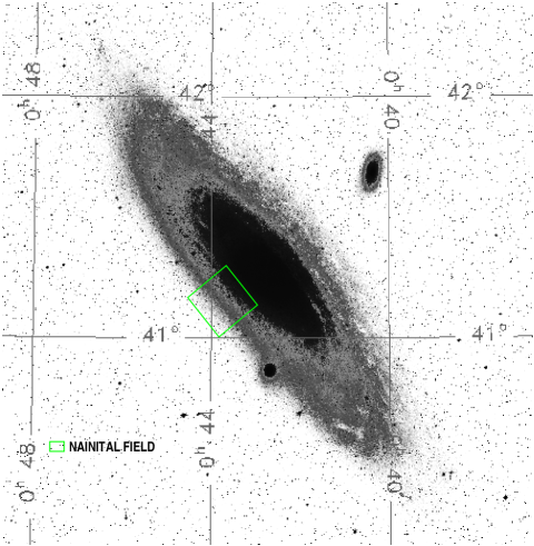
Figure 1: A $13^{\prime}\times 13^{\prime}$ field of Nainital Microlensing Survey juxtaposed over M31.

2 Observations

We started Cousins $R$ and $I$ band observations in the direction of M31 in 1998, with a small 1K$\times$1K CCD covering an area of $\sim 6^{\prime}\times 6^{\prime}$ at the f/13 Cassegrain focus of 104-cm Sampurnanand Telescope. Since 1999, observations have been carried out with a larger size 2K$\times$2K CCD chip which covers $\sim 13^{\prime}\times 13^{\prime}$ encompassing the previous field. Each pixel covers an area of 0.37$\times$0.37 arcsec² of the sky. The target field is centered at $\alpha_{2000}$ = $0^{h}43^{m}38^{s}$ and $\delta_{2000}$ = $+41^{\circ}09^{\prime}.1$, at a distance of about 15 arcmin in the South-East direction from the center of M31. Fig. 1 shows the location of the target field superposed over the image of M31. In the 4 year observing run, we accumulated a total of 468 data points in $R$ band and 383 data points in $I$ band during 141 observational nights spanning $\sim$ 1200 days. A histogram of the data taken in the survey is shown in Fig. 2. The average seeing during the observations was $\sim$ 2.2 arcsec. A detailed overview of the observations is given in Joshi et al. (2003).

Figure 2: A histogram of the data taken in the 4 year survey. The total number of nights observed per observing season is given in the box.

3 Pixel method

The basic principle of the pixel method is that if a star of flux $F_{*}$ is lensed in a crowded field, then by subtracting the original flux from the amplified flux of the star, one gets an increase in flux equal to $(A-1)F_{*}$ above the photon noise where $A$ is the magnification of star. Now if the target star shows a variation in the flux with time, it reflects in the $\Delta F$ of the pixel. Thus by following $\Delta F$ with time, we can monitor the variation in the flux of the target star. Although to detect any variation in the flux, this change should be significantly above the fluctuation level.

In the point-like lens and uniform motion approximation, the magnification factor $A$ is related to the impact parameter $u$ as given by the following Eq.

$$A(t)=\frac{u^{2}(t)+2}{u(t)\sqrt{u^{2}(t)+4}}$$ (1)

where $u^{2}(t)=u^{2}_{0}+\frac{(t-t_{0})^{2}}{t_{E}^{2}}$. Here $t_{0}$ and $t_{E}$ are the time of maximum amplification and Einstein time scale respectively and $u_{0}$ indicates the distance of closest approach in the units of Einstein radius. When $u(t)<<1$, the magnification is well approximated by

$$A(t)\equiv\frac{1}{u(t)};\leavevmode\nobreak\ \leavevmode\nobreak\ \leavevmode\nobreak\ \leavevmode\nobreak\ A_{max}\approx\frac{1}{u_{0}}$$

Then the change in flux of the target star is given by

$$\Delta F=\frac{F_{*}A_{max}}{\sqrt{1+\biggl{(}\frac{t-t_{0}}{t_{E}/A_{max}}\biggr{)}^{2}}}$$ (2)

From the light curve of a resolved star, one can get three parameters, namely peak time $(t_{0})$, Einstein time $(t_{E})$ and peak magnification $(A_{max})$ by fitting a theoretical light curve. However, for the unresolved stars as in the case of pixel lensing, there is a degeneracy between the $t_{E}$, $A_{max}$ and $F_{*}$ (Gould 1996). Hence, high quality data (e.g. Paulin-Henriksson et al. 2003) or detection of the source star (e.g. Auriére et al. 2001) are required to accurately determine the $t_{E}$ and hence the mass of the MACHO.

3.1 Implementation of the pixel method in Nainital data

Standard CCD reduction technique were used for the pre-processing of data using IRAF which includes bias subtraction, flat fielding and cosmic ray removal. We added all the frames of a particular filter taken on a single night and made one frame per filter per night to increase the signal to noise ratio.

3.1.1 Alignments

To align the images, we have to first select a reference frame taken in good photometric condition with lower sky background and relatively small seeing. We chose an image taken on January 05, 2000 as the reference frame. The average seeing during the night was 1.5 arcsec.

Since the observations were carried out on different nights, a star does not fall onto the same pixel in all the images. Therefore, we align all the images through rotation and shifting with respect to the reference frame. We achieve an accuracy better than 0.05 arcsec in alignment for most of the images.

Figure 3: Seeing distribution during the four year observing period.

The photometric conditions like the Earth’s atmospheric absorption and sky background are never the same for different nights. To bring all the images at same photometric level, we correct the images with respect to the reference frame using the statistical approach explained by Ansari et al. (1997). To overcome the residual gradient between two different frames due to reflected light, we normalize all the images with respect to the median background of the reference frame.

3.1.2 Seeing correction

Most of our observations were carried out in the early hours of the night when sky conditions might not have been perfectly stable, resulting in large seeing which is conspicuous in Fig. 3 where we have plotted the histogram of seeing variation with time in the four year observing run. The seeing during our observations varies in the range $\sim 1^{{}^{\prime\prime}}$.4 to 3${}^{{}^{\prime\prime}}$.2 with an average seeing of 2${}^{{}^{\prime\prime}}$.2. The large seeing fluctuations during different observing periods may cause a false variation in the pixel light curve. To correct it, we make a superpixel of $7\times 7$ pixel² ($\sim 2.5\times 2.5$ arcsec² area of sky) around each pixel so that most of the stellar flux falls on that superpixel although it only solves part of the seeing problem and does not correct

Figure 4: Linear correlation between the quantities $\Delta\phi_{tar}\equiv(\phi_{tar}-\tilde{\phi}_{tar})$ and $\Delta\phi_{ref}\equiv(\phi_{ref}-\tilde{\phi}_{ref})$. The left and right graphs show the correlation for the images of good $(1^{{}^{\prime\prime}}.4)$ and bad $(2^{{}^{\prime\prime}}.9)$ seeing. The seeing of the reference image is 1${}^{{}^{\prime\prime}}$.5. The dashed lines is the y = x line while the continuous lines indicate y = $\alpha$ x+$\beta$ line.

Figure 5: The variation of seeing correction coefficients $\alpha$ and $\beta$ as a function of seeing.

for the loss of photon counts in the changing wings of the PSF due to highly variable seeing between the frames. We thus correct the images by using the AGAPE ‘seeing stabilization method’ (Calchi Novati et al. 2002, Paulin-Henriksson et al. 2002) where we assume on the basis of empirical observations that the difference in flux between any image and its median background is linearly correlated to the same difference for the reference image i.e.

$$\phi_{i}-\tilde{\phi}_{i}=\alpha_{i}(\phi_{ref}-\tilde{\phi}_{ref})+\beta_{i}$$ (3)

where $\phi_{ref}$ and $\phi_{i}$ are the flux of reference and $i^{th}$ images respectively while $\tilde{\phi}_{ref}$ and $\tilde{\phi}_{i}$ are the flux of their respective median background images. The $\alpha_{i}$ and $\beta_{i}$ are the seeing correction coefficients for the $i^{th}$ image. In Fig. 4, we show the linear correlation between $(\phi_{ref}-\tilde{\phi}_{ref})$ and $(\phi_{curr}-\tilde{\phi}_{ref})$ for two images, one taken in good seeing and other one in bad seeing conditions. The $\alpha_{i}$ and $\beta_{i}$, which are calculated with a $\chi^{2}$ minimization procedure, shows a correlation with the seeing as shown in Fig. 5. After determining $\alpha$ and $\beta$ for each image, we correct them by

$$\phi_{i}^{new}=\frac{\phi_{i}-\tilde{\phi}_{i}-\beta_{i}}{\alpha_{i}}+\tilde{\phi}_{ref}$$ (4)

where $\phi_{i}^{new}$ is the modified flux after seeing correction. This correction scales all the images to the seeing of reference image.

3.2 Pixel light curves

To derive a pixel light curve, we mask bad pixels which are either bright stars for which photometric analysis has already been carried out or have contaminated due to spill-over of the saturated stars. In this way, we reject about 20% of the total pixels from the pixel analysis.

3.2.1 Stability of light curves

Since all the images are geometrically and photometrically aligned as well as seeing corrected, we expect the pixel light curve of non-variable objects to be stable with time. In Fig. 6, we illustrate the light curves of a stable pixel (782,579) in both $R$ and $I$ bands during its three year monitoring. The R.M.S. fluctuations along the light curve are $\sim$ 97 and $\sim$ 108 ADUs in $R$ and $I$ bands respectively which are less than the average error bars of $\sim$ 166 and $\sim$ 292 ADUs in the respective bands. This demonstrates that we have achieved a high level of stability in the pixel light curves after applying all the corrections.

Figure 6: The light curves of a non-varying pixel (782,579) in $R$ and $I$ bands during the 1999-2001 observing season.

3.2.2 Comparison: pixel vs photometric light curves

To check the robustness of the pixel technique for our data, we compare the pixel light curve of a star with its complementary light curve derived through the photometric technique. However, for the comparison, we cannot take a very bright star, where the seeing correction used in the pixel technique does not work well nor a very faint star where the photometric error in magnitude determination is too large. Therefore, we chose a Cepheid of $R=20.5$ mag having pixel coordinates (1186,595) for the comparison.

Figure 7: The $R$ band phase light curve of Cepheid (1186,595) derived with pixel and photometric techniques. Phase is plotted twice and in such a way that the minimum brightness falls at zero phase. The flux and the magnitude derived are not scaled.

From the data derived with pixel technique, we obtain a period of 7.457$\pm$0.002 days for the Cepheid using the period-searching program by Press & Rybici (1989). This value is in agreement with the period of 7.459$\pm$0.002 days determined by Joshi et al. (2003). This supports the robustness of the pixel technique implemented on our data. For a comparison, the phase light curves obtained by these two different techniques are shown in Fig. 7. Nevertheless, it is seen that the photometric technique is better for the resolved/bright stars while the pixel technique is ideally suited in the case of unresolved/faint stars.

4 Search for microlensing events

The pixel method relies on the monitoring of the flux variation of a pixel with time. To identify candidate pixels for the microlensing event, we adopt the same procedure as defined by Calchi Novati et al. (2002). Since $R$ band data have a better sampling density and photometric quality than that of the $I$ band data, we used only $R$ band data to select the light curves that are compatible with the microlensing event and $I$ band data will be used to analyse the microlensing candidate pixels. In the following sub-sections we briefly summarize the adopted procedure.

4.1 Selection criteria

Initially we define a base level which is the minimum value of the sliding average flux of 9 consecutive points on the light curve. We thereafter define a bump in the light curve as 3 consecutive points rise above the 3 sigma level and 2 consecutive points fall below the 3 sigma level. Since there is about a nine month gap between two consecutive observing seasons, we constrain all these points to be in the same observing run. For each bump, we define a likelihood function as

$$L=-ln\Big{(}\prod_{i\in bump}P(\phi>\phi_{i}|<\phi>_{i,\sigma_{i}})\Big{)}$$ (5)

where

$$P(\phi|\phi>\phi_{i})=\int_{\phi_{i}}^{\infty}\frac{1}{\sigma_{i}\sqrt{2\pi}}exp\big{[}-\frac{(\phi-\phi_{bkg})^{2}}{2\sigma_{i}^{2}}\big{]}d\phi$$

We chose only those pixels that have a primary bump with $L>300$ and no secondary bump with $L>70$ in the light curve. To exclude all those light curves that have more than one significant variation, we limit the ratio $\frac{L_{secondary}}{L_{primary}}$ to be not greater than 0.1. We find $\sim$ 19000 pixels that satisfy the above selection criteria. Most of them are clusters of pixels associated with significant physical variation. We cluster these pixels and select only those pixels that have the highest value of $L$ in their immediate neighbouring pixels. In this way we find 912 pixels characterized by the mono bump. To further check the flatness of the baseline of these pixels, we determine $\chi^{2}/N$ taking only those points which are used to determine baseline. A histogram of the $\chi^{2}/N$ for these pixels are shown in Fig. 8. To select the bumps

Figure 8: $\chi^{2}/N$ for the baseline flux. A vertical dashed line is drawn at $\chi^{2}/N=5$, above which all the pixels were rejected.

with a flat baseline, we reject all those pixels that have $\chi^{2}/N>5$. This selection reduces the pixels to only 670 that are used for the shape analysis test.

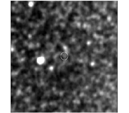
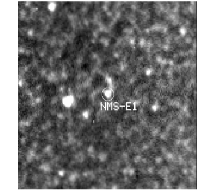
Figure 9: The position of NMS-E1 shown by the circle. The images are taken in $I$ band. The left frame shows no brightness at pixel (880,1402) while the right frame shows a resolved star at that position.

We do not enforce any selection criteria on $t_{1/2}$ as performed in some other surveys (e.g. Paulin-Henriksson et al. 2003, Riffeser et al. 2003) because of: $a)$ observational gaps in our data of up to 10 days between two consecutive nights within a single observing season; $b)$ the duration of the observations per season with an average observing density of once in three days; $c)$ the total period of our monitoring ($>800$ days)that is large enough to exclude any other kind of variability and $d)$ we are observing towards the outer disk of M31 where one generally expects long time scale events. Since the concentration of variable stars having longer period is higher as well as blending due to being greater seeing, microlensing candidates suffer from inhomogeneity in the light curve. We therefore explicitly check each light curve by eye and eliminates all those pixels having a periodic variability following Paulin-Henriksson et al. (2003). We further fit a 5-parameter Paczyński fit on the $R$ band data and a non-linear least squares fit estimated as

$$\chi^{2}=\sum_{i=1}^{n}\frac{\big{(}\phi(t_{i})-\phi_{fit}(t_{i})\big{)}^{2}}{\sigma^{2}(\phi(t_{i}))}$$

and determine the $\chi^{2}$ per degree of freedom ($\overline{\chi}^{2}$). We reject those light curves that has $\overline{\chi}^{2}>4$. This left us with 7 pixels. To further check the achromatism and symmetry in the selected pixels, we now use both $R$ and $I$ band data together. We find that 5 of them show significant variation in $I$ band while one of them shows no

Table 1: Selection criteria to determine microlensing candidates.

Condition	pixels left
Masking bad pixels	80%
Bump detection	$\sim$19000
Clustering of pixels	912
$(\chi^{2}/N)_{baseline}<5$	670
$\overline{\chi}^{2}<4$	7
7-parameter fit	1

synchronized variation in $R$ and $I$ bands as well as a large value of its half intensity duration hence needs further monitoring. This finally gives us one pixel which we have taken as a genuine microlensing candidate named as NMS-E1 where NMS is an acronym of the ‘Nainital Microlensing Survey’. A summary of the selection criteria is given in Table 1.

4.2 Microlensing Candidate NMS-E1

We find microlensing candidate NMS-E1 at the pixel coordinate (880,1402) corresponding to $\alpha_{2000}=00^{h}43^{m}33.3^{s},\delta_{2000}=+41^{\circ}06^{{}^{\prime}}44^{{}^{\prime\prime}}$ with an error of $\sim 1^{{}^{\prime\prime}}$ in both $\alpha$ and $\delta$. The candidate lies at an angular distance of $15^{{}^{\prime}}28^{{}^{\prime\prime}}$ on the far side of the disk from the M31 center and its position in our frames is shown in Fig. 9. The source is unresolved at its minimum brightness in our observations as can be seen to the left side of the figure, however, it is clearly visible when it reached its maximum brightness which is shown to the right side of the figure. The $R$ and $I$ band pixel light curves of NMS-E1 are shown in Fig. 10. A 7-parameter (i.e. full width at half maximum $t_{1/2}$, time of maximum amplification $t_{0}$, impact parameter $u_{0}$ and baseline flux and stellar flux for both the bands) Paczyński fit to the pixel light curves gives a half duration time of $t_{1/2}\sim 59\pm 2$ days with a peak magnification time of $t_{0}=1908\pm 1$ days.

Figure 10: The $R$ and $I$ band pixel light curves of NMS-E1 in the upper and lower panels respectively. The continuous lines represent the results of the 7-parameter Paczyński fit.

4.3 Shape analysis and achromaticity

A microlensing event possesses a characteristic Paczyński shape (Paczyński 1986) with a flat baseline and achromatic nature. The event NMS-E1 does not strictly follow symmetric shape as is evident from Fig. 10. It is seen that the shape of the light curve is broadened in $I$ band in comparison to the $R$ band.

When we have seen pixels around (880,1402), we find a bright source at $\sim 2^{{}^{\prime\prime}}.5$ to $\sim 5^{{}^{\prime\prime}}.5$ south-west that reach up to $R\sim$ 20.6 magnitude having a mean $(R-I)\sim 1.3$. Its photometric analysis indicates that the source could be a red variable. We did not find any other bright star in our observations at the detection limit of $R\sim 21.5$ mag. When we analyse the light curve of the same pixel in MDM data which is observed with the 1.3 m telescope and better seeing conditions, we see a bump in the light curve during the 1998-1999 observing season along with a few overlapping points in the rising branch of the microlensing candidate. We estimate the magnitude of the bump equivalent to

$$R(\Delta\phi)\sim 22.8;\leavevmode\nobreak\ \leavevmode\nobreak\ \leavevmode\nobreak\ \leavevmode\nobreak\ I(\Delta\phi)\sim 20.7$$

This star seems very close to the candidate pixel and cannot be resolved in our images. Although we cannot exactly estimate the magnitude of the star, its change in flux in the MDM light curve indicates that it is an extremely red variable. As each pixel of $\sim 2^{{}^{\prime\prime}}.5\times 2^{{}^{\prime\prime}}.5$ contains more than one thousand stars of M31, it is very likely that the nearby bright stars and red variables contaminate the pixel flux which not only deforms the shape of light curve but may also change the achromatic nature of the event.

Figure 11: Flux-flux variation of NMS-E1 where the x- and y-axis show the increase of flux in $R$ and $I$ bands respectively. The points around (0,0) indicate the base of the light curve. A continuous line indicates the best fit linear regression line.

To test the achromatic nature and effect of blending on the candidate event NMS-E1, we have drawn a flux-flux diagram in Fig. 11. The fit ($\chi^{2}/ndf=1.6$) is linear for the upper portion of the light curve within our noise level but it shows a systematic increase of flux in $\Delta(\phi_{I})$ around the fainter side of the microlensing regime which suggests that the light curve of NMS-E1, in general, is chromatic. However, keeping in mind the nearby red variable star contamination as we discussed earlier, it is not unexpected. In crowded regions like M31, it is quite difficult to separate out the noisy contribution from nearby variable sources. The effect of blending becomes more severe in the I band where the amplitude of variability is generally higher. The large and variable seeing in our observations further worsens the contamination problem. Most of the pixel lensing candidates towards M31 are severely contaminated by the nearby red variable stars which is also reflected in the various candidates reported by Calchi Novati et al. (2002, 2003), Paulin-Henriksson et al. (2002) and de Jong et al. (2003).

The physical parameters of NMS-E1 derived with the pixel technique as well its photometric analysis are summarized in Table 2.

Table 2: Characteristics of the event NMS-E1.

$\alpha$ (J2000)	$00^{h}43^{m}33.3^{s}$
$\delta$ (J2000)	$+41^{\circ}06^{{}^{\prime}}44^{{}^{\prime\prime}}$
distance from M31 center	$15^{{}^{\prime}}28^{{}^{\prime\prime}}$
$t_{0}$	1908$\pm$1
$t_{1/2}$	59$\pm$2 days
$R_{max}$	20.1 mag
$(R-I)$	1.3$\pm$0.2 mag
$\chi^{2}$/d.f	1.3

4.4 Physical interpretation of the event

We carry out photometry of NMS-E1 during its maximum brightness phase using DAOPHOT (Stetson 1987). The candidate reached its peak brightness in our observations on December 18, 1999 having magnitudes

$$R\sim 20.1;\leavevmode\nobreak\ \leavevmode\nobreak\ \leavevmode\nobreak\ \leavevmode\nobreak\ I\sim 18.8;\leavevmode\nobreak\ \leavevmode\nobreak\ \leavevmode\nobreak\ \leavevmode\nobreak\ (R-I)\sim 1.3$$

There can be an error of $\sim$ 0.2 mag in the colour determination. Assuming a distance modulus of $(m-M)_{0}=24.49$ and extinction of $A_{R}=0.63$, $A_{I}=0.47$ towards our observed direction of M31 (Joshi et al. 2003), we estimate

$$M_{R}=-5.0;\leavevmode\nobreak\ \leavevmode\nobreak\ \leavevmode\nobreak\ \leavevmode\nobreak\ M_{I}=-6.1;\leavevmode\nobreak\ \leavevmode\nobreak\ \leavevmode\nobreak\ \leavevmode\nobreak\ (R-I)_{0}=1.1$$

Figure 12: The position of NMS-E1 at its maximum brightness in the H-R diagram. The solar metallicity isochrones by Bertelli et al. (1994) for log $A$ = 7.5, 8.0 and 9.0 are also plotted. A vertical line is drawn to show the magnification direction.

The position of NMS-E1 in the H-R diagram is shown in Fig. 12. We can see that NMS-E1 is a very bright red star at its peak brightness which suggests that the source must lie either on the giant branch or it must be a M1-type main sequence (MS) star. If it is a MS star, its colour corresponds to an absolute magnitude of $M_{R}\sim 8$ mag (Cassisi et al. 1998) hence needs a very high magnification ($A_{max}>10^{5}$) to reach a brightness of $M_{R}>-5$ mag. Since NMS-E1 is a long time scale event, the latter possibility is less likely. If it is a red giant star then we should be able to detect it in the Hubble Space Telescope (HST) images as HST is capable of detecting giant branch stars in M31. Unfortunately, there are no observations available for this region in the HST archive. Although NMS-E1 is a long time scale event and red in colour, it is very unlikely that it is a Mira or any other long period variable as this event has been monitored for more than 800 days. This is one of the few pixel lensing events reported so far that has been tracked for such a long duration that allowed us to rule out any possibility of it being a variable star.

Microlensing events that occur due to the objects in the halo of M31 generally have a longer time scale than the stars in the bulge or disk of M31 due to the observer-lens-source geometry (Baltz et al. 2003). The high value of $t_{1/2}$ of NMS-E1 as well as its location on the far side of the M31 disk indicate that the event might be due to halo lensing. The MEGA collaboration has also reported two long time scale microlensing candidates in the disk of M31 using the differential technique i.e. ML-10 and ML-12 with the durations of $t_{1/2}\sim 47$ and 133 days respectively (de Jong et al. 2003). The candidate ML-10 lies in our observed field at an angular distance of $\sim 6^{{}^{\prime}}.6$ from the position of NMS-E1 but shows a stable light curve in our data since we started observations when this event had almost merged with the background noise.

5 Discussion and conclusions

The main difficulty with the pixel lensing search, in contrast to the conventional microlensing search, is that one cannot usually be able to measure the Einstein time $t_{E}$ of the event from the observed pixel light curve which carries most of the physical information on the MACHO population. This is because the flux of a normally unresolved star in the absence of the lensing is unknown. There is however one event, PA-99-N1 reported by the POINT-AGAPE collaboration (Auriére et al. 2001, Paulin-Henrisksson et al. 2003), where an unlensed star has been identified in HST archival images. We lack such identification in the present study. Since we could not identify the source star, it is not possible for us to determine $t_{E}$ and hence the mass of the lens. Nevertheless, by proper modeling of the stellar populations which either can be source stars or lens objects, we can estimate various parameters like the timescale of microlensing events, their rate of occurrence or spatial distribution (de Jong et al. 2003). However, we need to detect a reasonable sample of genuine microlensing events along with prior knowledge of the detection efficiency before making any conclusive estimates.

We have reported our first microlensing candidate detected with the pixel technique on the far side of the galactic disk of M31. The peak brightness of the candidate $R_{max}\sim 20.1$ mag coupled with its colour $(R-I)_{0}\sim 1.1$ and half intensity duration of $t_{1/2}\sim 59$ days lends support to it being a red giant source while it being main sequence star is highly improbable. The half intensity duration along with its location in M31 suggest that the event NMS-E1 might be due to halo lensing. Since we still have not estimated the detection efficiency, the likelihood of the event and results of Monte Carlo simulations will be discussed in a future publication. The variable stars of M31 have also been the subject of numerous studies e.g. star formation history, stellar population etc.; we are trying to compile a catalogue of pixel variables in our target field.

Here we presented the results of the pilot observational campaign carried out towards M31. We have been continuing our observations of the same field using the new 2-m Himalayan Chandra Telescope (HCT), Hanle, India and we expect to find a larger number of events which may enlighten us on the dark matter problem in the galactic halos of M31 and our own galaxy.

Acknowledgments   We would like to thank B. Paczyński for his constructive comments which improved this paper. It is a great pleasure to thank Yannick Giraud-Héraud and Jean Kaplan for their kind support in initiating the project and helping us to get familiar with the pixel technique. DN is grateful to Japan Society for the Promotion of Science for an Invitation Fellowship. This study is a part of the project 2404-3 supported by the Indo-French center for the Promotion of Advanced Research, New Delhi.

References

- (1) Alard, C., & Lupton R. H., 1998, ApJ, 503, 325
- (2) Alard, C., 2000, A&AS, 144, 363
- (3) Alcock, C., Akerlof, C. W., Allsman, R. A., et al., 1993, Nature, 365, 621
- (4) Alcock, C., Allsman, R. A., Alves, D. R., et al., 2000, ApJ, 542, 281
- (5) Ansari, R., Aurière, M., Baillon, P., et al., 1997, A&A, 324, 843
- (6) Aubourg, E., Bareyre, P., Brehin, S., et al., 1993, Nature, 365, 623
- (7) Aurière, M., Baillon, P., Bouquet, A., et al., 2001, ApJ, 553, L137
- (8) Bonanos, A. Z., Stanek, K. Z., Sasselov, D. D., et al., 2003, AJ, 126, 175
- (9) Baillon, P., Bouquet, A., Kaplan, J., & Giraud-Héraud, Y., 1993, A&A, 277, 1
- (10) Baltz, E. A., Gyuk, G., & Crotts, A. P. S., 2003, ApJ, 582, 30
- (11) Bertelli, G., Bressan, A., Chiosi, C., Fagotto, F., & Nasi, E., 1994, A&AS, 106, 275
- (12) Calchi Novati, S., Iovane, G., Marino, A. A., et al., 2002, A&A, 381, 848
- (13) Calchi Novati, S., Jetzer, Ph., Scarpetta, G., et al., 2003, A&A, 405, 851
- (14) Cassisi, S., Castellani, V., degl’Innocenti, S., & Weiss, A. 1998, A&AS, 129, 267
- (15) Crotts, A. P. S., 1992, ApJ, 395, L25.
- (16) Tomaney, A. B., & Crotts, A. P. S., 1996, AJ, 112, 2872
- (17) de Jong, J. T. A., Kuijken, K. H., Crotts, A. P. S., et al., 2003, A&A, 417, 461
- (18) Gould, A., 1996, ApJ, 470, 201
- (19) Joshi, Y. C., Pandey, A. K., Narasimha, D., Sagar, R., & Giraud-Héraud, Y., 2003, A&A, 402, 113
- (20) Joshi, Y. C., 2004, Ph.D Thesis, Kumaon University, Nainital, India
- (21) Lasserre, T., Afonso, C., Albert, J. N., et al., 2000, A&A, 355, L39
- (22) Paczyński, B., 1986, ApJ, 304, 1.
- (23) Paulin-Henriksson, S., Baillon, P., Bouquet, A., et al., 2002, ApJ, 576, L121
- (24) Paulin-Henriksson, S., Baillon, P., Bouquet, A., et al., 2003, A&A, 405, 15
- (25) Press, W. H., & Rybici, G. B., 1989, ApJ, 338, 277
- (26) Riffeser, A., Fliri, J, Bender, R., et al., 2003 ApJ, 599, L17.
- (27) Stetson, B., 1987, PASP, 99, 191.
- (28) Stanek, K. Z., & Garnavich, O. M., 1998, ApJ, 503, L131
- (29) Taylor, S. F., 2004, PASP, 116, 1126
- (30) Udalski, A., Szymanski, M., Kaluzny, J., et al., 1993, Acta Astron., 43, 289