CMB lensing extraction and primordial non-Gaussianity

Abstract

The next generation of CMB experiments should get a better handle on cosmological parameters by mapping the weak lensing deflection field, which is separable from primary anisotropies thanks to the non-Gaussianity induced by lensing. However, the generation of perturbations in the Early Universe also produces a level of non-Gaussianity which is known to be small, but can contribute to the anisotropy trispectrum at the same level as lensing. In this work, we study whether the primordial non-Gaussianity can mask the lensing statistics. We concentrate only on the “temperature quadratic estimator” of lensing, which will be nearly optimal for the Planck satellite, and work in the flat-sky approximation. We find that primordial non-Gaussianity contaminates the deflection field estimator by roughly $(0.1f_{NL})$% at large angular scales, which represents at most a 10% contribution, not sufficient to threaten lensing extraction, but enough to be taken into account.

Introduction – Cosmic Microwave Background (CMB) anisotropies are of considerable interest for cosmology because after cleaning the observed temperature and polarization maps from various foregrounds, one obtains a picture of cosmological perturbations on our last-scattering surface. The power spectra of primary anisotropies are related to various cosmological parameters, and depend on the physical evolution mainly before the time of decoupling (and also, more weakly, on its recent evolution, through the integrated Sachs-Wolfe effect and the angular diameter–redshift relation).

It was realized recently that CMB anisotropies encode even more cosmological information than expected, because it should be possible in a near future to measure the deflection field caused by the weak lensing of CMB photons by the large scale structure of the neighboring universe at typical redshifts $z\sim 3$ Ber97 ; LE . The power spectrum of the deflection field encodes some information concerning structure formation mainly in the linear or quasi-linear regime, and is therefore extremely useful for measuring parameters like the total neutrino mass or the dark energy equation-of-state, which mildly affect the primary anisotropy Kap03 . So, the next generation of CMB experiments could output for free a Large Scale Structure (LSS) power spectrum, without suffering like galaxy redshift surveys from the systematics induced by mass-to-light bias and by strong non-linear corrections on small scales at $z\leq 0.2$.

There are several methods on the market for extracting the deflection map QE1 ; QE2 ; QE3 ; IE , all based on the non-Gaussianity induced by lensing Ber97 . These methods start from the assumption that both the primary anisotropies and the deflection field are Gaussian; they also assume that the noise present in the temperature and polarization maps is Gaussian and uncorrelated with the signal.

None of these assumptions is exactly true. Amblard et al. Amb04 already estimated to which extent the lensing extraction will be biased, first, by the non-Gaussianity of the lensing potential caused by the non-linear growth of matter perturbations on small scales, and second, by the imperfect cleaning of the CMB maps from the kinetic Sunyaev-Zel’dovich effect, which also has a blackbody spectrum, induces non-Gaussianity, and features spatial correlations with many of the structures responsible for the lensing. Both effects were found to be relevant (i.e., to induce a significant bias in the estimators). However, they are small enough to preserve the validity of the method.

The purpose of this work is to relax the first of the previous assumptions, and to consider realistic situations, in which one cannot avoid a small level of non-Gaussianity to be produced in the Early Universe. Non-Gaussianity emerges as a key observable to discriminate among competing scenarios for the generation of cosmological perturbations and is one of the primary targets of present and future CMB satellite missions NG . Indeed, despite the simplicity of the inflationary paradigm reviewlr , the mechanism by which cosmological curvature perturbations are generated is not yet established. In the standard slow-roll scenario associated to one-single field models of inflation, the observed density perturbations are due to fluctuations of the inflaton field itself when it slowly rolls down along its potential. In the curvaton mechanism curvaton the final curvature perturbation is produced from an initial isocurvature perturbation associated with the quantum fluctuations of a light scalar field (other than the inflaton), the curvaton, whose energy density is negligible during inflation. Recently, other mechanisms for the generation of cosmological perturbations have been proposed, the inhomogeneous reheating scenario gamma1 , the ghost inflationary scenario ghost , and the D-cceleration scenario dacc , just to mention a few. Single-field slow-roll inflationary model inflation itself produces a negligible amount of non-Gaussianity, and the dominant contribution comes from the evolution of the ubiquitous second-order perturbations after inflation. However, alternative models for the generation of perturbations might produce much stronger primordial non-Gaussianity. Therefore, non-Gaussianity in the CMB maps from primordial fluctuations could mask the non-Gaussianity from lensing distortions. We will see later that if one expands the power spectrum of the lensing estimator in powers of the gravitational potential $\Phi\sim 10^{-5}$, the contribution from primordial non-Gaussianity appears at the same order as the lensing power spectrum itself. Therefore, a precise computation is needed in order to understand whether the primordial non-Gaussianity could affect lensing extraction.

Lensing extraction with quadratic estimators – Weak lensing induces a deflection field ${\bf d}$, i.e., a mapping between the direction of a given point on the last scattering surface and the direction in which we observe it. At leading order IE this deflection field can be written as the gradient a lensing potential, ${\bf d}=\nabla\phi$.

In the limit of Gaussian primordial fluctuations, the unlensed anisotropies obey Gaussian statistics, and in the flat-sky approximation their two-dimensional Fourier modes are fully described by the power spectra $\tilde{C}^{ab}_{l}$ where $a$ and $b$ belong to the $\{T,E,B\}$ basis. Weak lensing correlates the lensed multipoles Sel96 ; Ber97 according to

$$\langle a({\bf l})b({\bf l^{\prime}})\rangle_{\rm CMB}=(2\pi)^{2}\delta({\bf l}+{\bf l^{\prime}})\tilde{C}^{ab}_{l}+f^{ab}({\bf l},{\bf l^{\prime}})\phi({\bf l}+{\bf l^{\prime}})$$ (1)

where the average holds over different realizations (or different Hubble patches) of a given cosmological model with fixed primordial spectrum and background evolution (i.e. fixed cosmological parameters). In this average, the lensing potential is also kept fixed by convention, which makes sense because the CMB anisotropies and LSS that we observe in our past light-cone are statistically independent, at least as long as we neglect the integrated Sachs-Wolfe effect. The above function $f^{ab}$ is defined in QE2 and takes a simple form in the case $ab=TT$:

$$f^{TT}({\bf l},{\bf l^{\prime}})=C^{TT}_{l}({\bf l}+{\bf l^{\prime}})\cdot{\bf l}+C^{TT}_{l^{\prime}}({\bf l}+{\bf l^{\prime}})\cdot{\bf l}^{\prime}~{}.$$ (2)

Our study will be based on the quadratic estimator method of Hu & Okamoto QE1 ; QE2 ; QE3 (which is equivalent in terms of precision to the alternative iterative estimator method of Hirata & Seljak IE as long as CMB experiments will make noise-dominated measurements of the B-mode, i.e., at least for the next decade). By inverting Eq. (1), one builds a quadratic combination of the temperature and polarization observed Fourier modes

$${\bf d}^{ab}({\bf L})=\frac{i{\bf L}A^{ab}_{L}}{L^{2}}\int\!\!\!\frac{d^{2}{\bf l}_{1}}{(2\pi)^{2}}a({\bf l_{1}})b({\bf l_{2}})g^{ab}({\bf l_{1}},{\bf l_{2}})$$ (3)

where ${\bf l_{2}}={\bf L}-{\bf l_{1}}$, and in which the normalization condition

$$A^{ab}_{L}=L^{2}\left[\frac{d^{2}{\bf l}_{1}}{(2\pi)^{2}}f_{TT}({\bf l}_{1},{\bf l}_{2})g^{ab}({\bf l}_{1},{\bf l}_{2})\right]^{-1}$$ (4)

ensures that ${\bf d}^{ab}$ is an unbiased estimator of the lensing potential:

$$\langle{\bf d}^{ab}({\bf L})\rangle_{\rm CMB}=i{\bf L}\phi({\bf L})={\bf d}({\bf L})~{}.$$ (5)

Note that, so far, the coefficients $g^{ab}({\bf l}_{1},{\bf l}_{2})$ are still arbitrary. From the observed temperature and polarization maps, one could compute each mode of ${\bf d}^{ab}$ and obtain various estimates of the deflection modes, precise up to cosmic variance and experimental errors. In order to quantify the total error, it is necessary to compute the power spectra of the quadratic estimators

$$\langle{\bf d}^{ab*}({\bf L}){\bf d}^{ab}({\bf L})\rangle=(2\pi)^{2}\delta({\bf L}-{\bf L}^{\prime})C_{L}^{dd(ab)}$$ (6)

where the average is now taken over both CMB and LSS realizations, since $\phi({\bf L})$ is also a stochastic quantity. In this definition, the power spectra are written with a superscript $dd(ab)$ in order to be distinguished from the actual power spectrum of the true deflection field. These spectra feature the four-point correlation function of the observed (lensed) Fourier modes $\langle a({\bf l}_{1})b({\bf l}_{2})a({\bf l}_{3})b({\bf l}_{4})\rangle$, which should be expanded at order two in $\phi({\bf L})$ in order to catch the leading non-Gaussian contribution.

The four-point correlation functions are composed as usual of a connected and an unconnected piece. The connected piece is by definition a function of the power spectra $C_{l}^{ab}$ in which we now include all sources of variance: cosmic variance, lensing contribution and experimental noise. The unconnected piece is a function of the same spectra plus the deflection spectrum $C_{l}^{dd}$, and as usual it can be decomposed in three terms corresponding to the different pairings of the four indices TRI1 : $(l_{1},l_{2})$, $(l_{3},l_{4})$ or $(l_{1},l_{3})$, $(l_{2},l_{4})$ or $(l_{1},l_{4})$, $(l_{3},l_{2})$. The first term leads to considerable simplifications when it is plugged into the expression of the quadratic estimator power spectrum, and the result is simply $C_{l}^{dd}$, as one would expect naively from squaring Eq. (5). The other terms lead to more complicated expressions that we will write as two noise terms:

$$C_{L}^{dd(ab)}=C_{L}^{dd}+[N_{\rm c}]^{ab}_{L}+N^{ab}_{L}~{},$$ (7)

which represent respectively the contribution from the connected piece and from the two non-trivial terms of the unconnected piece TRI1 ; Coo02 (later, we will give the exact expressions in the case $aa=TT$). In order to get an efficient estimator, we should adopt the set of coefficients $g^{ab}({\bf l}_{1},{\bf l}_{2})$ which minimize the noise terms. It is actually much easier to minimize the connected term only, which leads to the simple results

$$g^{aa}({\bf l}_{1},{\bf l}_{2})=\frac{f_{aa}({\bf l},{\bf l}^{\prime})}{2C_{l}^{aa}C_{l^{\prime}}^{aa}}\quad{\rm and}\quad[N_{\rm c}]^{aa}_{L}=A^{aa}_{L}$$ (8)

for $a\!=\!b$ (for $a\!\neq\!b$ see QE2 ). With such a choice, the unconnected piece contribution $N^{ab}_{L}$ can be shown to be smaller than $A^{aa}_{L}$, but not completely negligible Coo02 .

The various estimators ${\bf d}^{ab}$ can be constructed for each pair of modes, except for the pair $BB$, because the spectrum $C_{l}^{BB}$ is dominated by lensing at least on small scales, which invalidates the present method. So, the quadratic estimator technique would not be optimal for long-term CMB experiments with cosmic-variance-dominated measurement of the $B$ mode IE ; Smi04 . For an experiment of given sensitivity, the five other estimators can be combined into a final minimum variance estimator, which gives the best possible estimate of the deflection field by weighing each estimator accordingly to its noise level. The sensitivity of the Planck satellite Planck is slightly above the threshold for successful lensing extraction, but only at intermediate angular scales, and with essentially all the signal coming from the ${\bf d}^{TT}$ estimator. The following generation of experiments – such as the CMBpol or Inflation probe project CMBpol – should obtain the lowest noise level from the ${\bf d}^{EB}$ estimator QE2 .

We summarized here the quadratic estimator method, which assumes that both the primary anisotropies and the lensing potential are Gaussian. We will now study the impact of primordial non-Gaussianity. This program is numerically cumbersome, and we will only concentrate on the ${\bf d}^{TT}$ estimator, which is the only relevant one for Planck, while sticking to the flat-sky approximation in which numerical computations are much quicker.

Contributions from primordial non-Gaussianity – The two-dimensional Fourier modes of both temperature anisotropies and the lensing potential can be related to the stochastic three-dimensional modes of the primordial gravitational potential $\Phi({\bf k})$, multiplied by a transfer function which accounts for its time-evolution. The fact of writing a unique stochastic function can bring some confusion, because the modes $\Phi({\bf k})$ which appear in the CMB and lensing expressions represent fluctuations at very different redshifts: the first ones before decoupling, the second at $z\sim 3$, i.e. in the neighboring universe. So, as long as we neglect the integrated Sachs-Wolfe effect, it is convenient to introduce two statistically independent functions $\Phi^{\rm CMB}({\bf k})$ and $\Phi^{\rm LSS}({\bf k})$, sharing the same statistical properties, but sourcing respectively $a({\bf l})$ and $\phi({\bf l})$.

The true non-Gaussian potential $\Phi^{\rm X}_{NL}$ (x = cmb or lss) can be expanded in real space in powers of a Gaussian potential $\Phi^{\rm X}_{L}$. In Fourier space and at order three,

$$\Phi^{X}_{NL}({\bf k})=\Phi^{X}_{L}({\bf k})+\Phi^{X}_{A}({\bf k})+\Phi^{X}_{B}({\bf k})$$ (9)

with

$$\Phi^{X}_{A}({\bf k})\!\!\! = \!\!\!f_{NL}\!\left[\int\!\!\frac{d^{3}{\bf p}}{(2\pi)^{3}}\Phi^{X}_{L}({\bf k\!+\!p})\Phi^{X*}_{L}({\bf p})\!-\!(2\pi)^{3}\delta({\bf k})\overline{\Phi^{2}_{L}}\right]$$

$$\Phi^{X}_{B}\!({\bf k})\!\!\! = \!\!\!g_{NL}\!\!\int\!\!\!\frac{d^{3}{\bf p}_{1}}{(2\pi)^{3}}\!\frac{d^{3}{\bf p}_{2}}{(2\pi)^{3}}\Phi^{X*}_{L}\!({\bf p_{1}})\Phi^{X*}_{L}\!({\bf p_{2}})\Phi^{X}_{L}\!({\bf p_{1}\!\!+\!\!p_{2}\!\!+\!\!k})$$

$${\rm and}~{} \overline{\Phi^{2}_{L}}=\int\frac{d^{3}{\bf k}}{(2\pi)^{3}}P_{\Phi}(k)~{}.$$

We have parametrized the primordial non-Gaussianity by a quadratic and a cubic term in the gravitational potential. They are proportional to the dimensionless parameters $f_{\rm NL}$ and $g_{\rm NL}$, respectively. The theoretically predicted parameter $f_{\rm NL}$ appears as a kernel in Fourier space, rather than a constant, in most of the scenarios for the generation of the cosmological perturbations, while theoretical predictions for the parameter $g_{\rm NL}$ are still lacking . This gives rise to an angular modulation of the quadratic non-linearity, which might be used to search for specific signatures of inflationary non-Gaussianity in the CMB. In this paper, however, we restrict ourselves to the simplest case and assume $f_{\rm NL}$ and $g_{\rm NL}$ as mere phenomenological multiplicative constants. Under this assumption, the WMAP team has measured the bispectrum to obtain the tightest limit to date, $-58<f_{\rm NL}<134$ ($95\%$) k . On the other hand, no observational bound has been set on $g_{\rm NL}$ from the observed trispectrum. However, one can simply notice from Eq. (9) that the small parameter $(f_{\rm NL}\Phi)$ contributes at the same order as $(\sqrt{g_{\rm NL}}~{}\Phi)$: so, by comparing with the $f_{\rm NL}$ bound, it is likely that values of order $\sqrt{g_{\rm NL}}\sim 100$ are still allowed by the data.

As far as lower bounds are concerned, one should keep in mind that although single-field slow-roll inflation itself produces a negligible amount of non-Gaussianity, the dominant contribution comes from the evolution of the ubiquitous second-order perturbations after inflation. This effect must exist regardless of the inflationary model, setting the minimum level of non-Gaussianity in the cosmological perturbations at order $f_{\rm NL}\!\sim\!g_{NL}\!\sim\!1$.

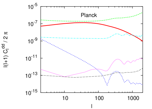
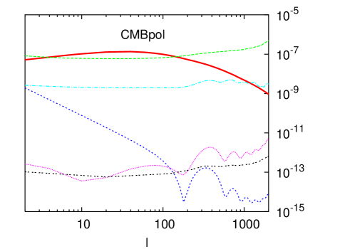
Figure 1: Various contributions to the variance of a single mode of the estimator ${\bf d}^{TT}({\bf l})$, for the case of Planck (left) and CMBpol (right). The thick (red) curve shows the variance of the signal $C_{l}^{dd}$. Other curves represent (from top to bottom at $l\!\sim\!2000$) the noise variance from the connected part of the four-point correlation function, from the lensing trispectrum, and from the terms $B$, $A2$ and $A1$ in the primordial non-Gaussianity trispectrum (displayed for $f_{NL}\!=\!g_{NL}^{1/2}\!=\!100$).

In order to evaluate the impact of these extra contributions on the power spectrum $C_{L}^{dd(a,b)}$, we should first recompute the four-point functions $\langle a_{l_{1}}^{m_{1}}b_{l_{2}}^{m_{2}}a_{l_{3}}^{m_{3}}b_{l_{4}}^{m_{4}}\rangle$, working as before at order six in the gravitational potential. Non-zero contributions can arise only from terms with an even number of $\Phi^{\rm CMB}_{L}({\bf k})$ and $\Phi^{\rm LSS}_{L}({\bf k})$ factors. The standard calculation of the previous section included terms in which either two multipoles were lensed at order one in $\phi({\bf l})$, or one multipole was lensed at order two (the later terms contributes only to the connected piece). In addition, we should now consider terms in which:

• the four multipoles are unlensed, but two of them include the term $\Phi^{\rm CMB}_{A}$,

• the four multipoles are unlensed, one of them includes the term $\Phi^{\rm CMB}_{B}$,

• one of the four multipoles is lensed at order one in $\phi({\bf l})$, which includes the term $\phi^{\rm LSS}_{A}$.

The last term C vanishes because $\phi^{\rm LSS}_{A}$ has zero average. So, at leading order, lensing and primordial non-Gaussianity effects are completely separable, and we simply need to add corrections from the primordial non-Gaussianity trispectrum, which is given in Okamoto & Hu TRI2 (who computed it in the Sachs-Wolfe approximation). First, one needs to compute the integrals

$$F_{l}(r_{1},r_{2}) = \frac{2}{\pi}\int k^{2}dk\,P_{\Phi}(k)j_{l}(kr_{1})j_{l}(kr_{2})~{},$$ (10)

$$\alpha_{l}(r) = \frac{2}{\pi}\int k^{2}dk\,\Delta_{l}(k)j_{l}(kr)~{},$$ (11)

$$\beta_{l}(r) = \frac{2}{\pi}\int k^{2}dk\,P_{\Phi}(k)\Delta_{l}(k)j_{l}(kr)~{},$$ (12)

where $\Delta_{l}(k)$ is the radiation transfer function for the temperature, normalized to $\Phi\!=\!1$ in the early universe. We checked that our functions $\alpha_{l}(r)$ and $\beta_{l}(r)$ (computed with a slightmy modified version of cmbfast CMBFAST ) perfectly agree with those of Kom01 . Each of the $A$ and $B$-type trispectra are composed of three parts, which can be simply expressed in terms of the intermediate quantities

$$(P_{A})^{{l_{1}}{l_{2}}}_{{l_{3}}{l_{4}}} \!\!\!(L)=4f_{1}^{2}\!\!\!\int\!\!r_{1}^{2}dr_{1}\!\!\int\!\!r_{2}^{2}dr_{2}\,F_{L}(r_{1},r_{2})\times$$

$$\,\,\,\,\,\,\left[\alpha_{l_{1}}\!(r_{1})\beta_{l_{2}}\!(r_{1})+{\rm c.p.}\right]\left[\alpha_{l_{3}}\!(r_{2})\beta_{l_{4}}\!(r_{2})+{\rm c.p.}\right]~{},$$

$$(P_{B})^{{l_{1}}{l_{2}}}_{{l_{3}}{l_{4}}} \!\!=2f_{2}\!\!\int\!\!r^{2}dr\left[\alpha_{l_{1}}\!(r)\beta_{l_{2}}\!(r)\beta_{l_{3}}\!(r)\beta_{l_{4}}\!(r)+{\rm c.p.}\right]~{},$$

where c.p. means circular permutation of the indices $l_{i}$. The final expression for the power spectrum of the quadratic estimator for any mode ${\bf L}$ of modulus $L$, including the three trispectra induced by lensing and primordial non-Gaussianity, reads

$$C_{L}^{dd(TT)}\!=C_{L}^{dd}+A_{L}^{TT}$$

$$+\frac{{A^{TT}_{L}}^{2}}{L^{2}}\!\!\int\!\!\!\frac{d^{2}{\bf l}_{1}}{(2\pi)^{2}}\!\frac{d^{2}{\bf l}^{\prime}_{1}}{(2\pi)^{2}}g^{TT}\!({\bf l}_{1},\!{\bf l}_{2})g^{TT}\!({\bf l}^{\prime}_{1},\!{\bf l}^{\prime}_{2})\times$$

$$\left[2\,|{\bf l}_{1}\!-{\bf l}^{\prime}_{1}|^{-2}C_{|{\bf l}_{1}-{\bf l}^{\prime}_{1}|}^{dd}f^{TT}({\bf l}_{1},\!-{\bf l}^{\prime}_{1})f^{TT}({\bf l}_{2},\!-{\bf l}^{\prime}_{2})\right.$$

$$\left.+(P_{A})^{{l_{1}}{l_{2}}}_{{l^{\prime}_{1}}{l^{\prime}_{2}}}(L)+2(P_{A})^{{l_{1}}{l^{\prime}_{1}}}_{{l_{2}}{l^{\prime}_{2}}}(|{\bf l}_{1}-{\bf l}^{\prime}_{1}|)+3(P_{B})^{{l_{1}}{l_{2}}}_{{l^{\prime}_{1}}{l^{\prime}_{2}}}\right]~{}~{}~{}~{}~{}~{}~{}~{}$$ (13)

with ${\bf l}_{2}={\bf L}-{\bf l}_{1}$ and ${\bf l}^{\prime}_{2}={\bf L}-{\bf l}^{\prime}_{1}$. The variance of the signal $C_{L}^{dd}$ comes from the first term of the lensing trispectrum, while the noise variance $A_{L}^{TT}$ comes from the connected part of the four-point correlation function. We can identify all the other sources of noise inside the integral. The third line of Eq. (13) contains the two other terms of the lensing trispectrum, which give equal contributions (as can be shown after a change of variable). The last line contains the three terms of the $A$-type trispectrum (the last two contribute equally) and the three terms of the $B$-type trispectrum (three equal contributions). Let us call $A1$, $A2$ and $B$ the terms of the last line.

The numerical integration of Eq. (13) could be exceedingly long, due to the four-dimensional integral in Fourier space (which converges only when the upper bound of integration is taken around the Silk-damping cut-off, $l_{\rm max}\sim 2500$) and of the two-dimensional integral in $r$ space. Fortunately, the second integral can be limited to values of $r$ close to the comoving distance to the last-scattering surface, far from which $r^{2}\alpha_{l}(r)$ is negligible. Here, we will integrate $r=\tau_{0}-\tau$ from $0.03\tau_{*}$ to $1.3\tau_{*}$ with a conservative step $d\tau=0.01\tau_{*}$ (where $\tau$ stands for conformal time, $\tau_{0}$ is evaluated today, and $\tau_{*}$ is the conformal time at recombination, defined as the peak of the visibility function).

The integration in $l$-space can be sped up by taking into account various symmetries, and also by noting that for the terms $A1$ and $B$ the integral over ${\bf l}_{1}$ and ${\bf l}_{1}^{\prime}$ are separable. Then, the integration effectively reduces to a two-dimensional one. For these terms, we integrate first on ${\bf l}_{1}$, then on $r_{1}$ and $r_{2}$, and obtain the full result in few minutes. The term $A2$ and the lensing term require a real four-dimensional integral and more CPU time. Fortunately, the quantities to integrate are very smooth in $l$-space, and one can considerably reduce the computing time by choosing a large step without loosing precision. We checked that $\Delta l\sim 30$ is by far sufficient.

Results and conclusions – We take a fiducial $\Lambda$CDM model with $\Omega_{b}\!=\!0.05$, $\Omega_{c}\!=\!0.25$, $\Omega_{\Lambda}\!=\!0.70$, $h\!=\!0.65$, no reionization and a scale-invariant primordial spectrum $P_{\Phi}(k)\!=\!6.204\times 10^{-11}k^{-3}$. For instrumental noise, we consider the cases of Planck HFI (three channels) and of the CMBpol project, with a sensitivity described by the same parameters as in LPP . We show in Fig. 1 the various contributions to the estimator power spectrum, as computed from Eq. (13). Note that we are plotting the variance of a single mode ${\bf l}$, and not the error on the reconstructed deflection power spectrum, which can be lowered by combining all modes of given wavenumber $l$ and by binning the data (this is why Planck is likely to make a reasonable detection of the deflection power spectrum at intermediate $l$’s QE2 , although the noise variance is slightly larger than the signal variance in Fig. 1). The contributions from the primordial non-Gaussianity terms $A$ and $B$ scale respectively like $f_{NL}^{2}$ and $g_{NL}$, and here they are shown for $f_{NL}^{\phantom{1}}\!=\!\sqrt{g_{NL}}\!=\!100$.

The contamination from primordial non-Gaussianity appears to arise mainly at low $l$, from the $A1$-type term. On these scales it would be necessary to perform an exact all-sky computation in order to make a precise prediction. However, the error caused by the flat-sky approximation even at low $l$ is usually small TRI1 .

The noise induced by primordial non-Gaussianity is responsible for roughly $(0.1f_{NL})$% of the amplitude of the estimator ${\bf d}^{TT}({\bf l})$ in the range $2<l<10$: so, around 10% for the largest possible value of $f_{NL}$, and around 0.1% for standard slow-roll inflationary models. In the range $100<l<1000$, the contribution is roughly of order $(10^{-3}f_{NL})$% from the $A2$ term, and $(0.01\sqrt{g_{NL}})$% from the $B$ term.

If in the near future $f_{NL}$ appears to be large, it will be measured independently using the three-point correlation function. It should then be possible to subtract to some extent the bias induced by primordial non-Gaussianity when reconstructing the power spectrum $C_{L}^{dd}$, as suggested in Coo03 ; Amb04 for other sources of bias.

We conclude that primordial non-Gaussianity should be taken into account if it is as large as to saturate the present upper bounds, but that in no case it will represent a dangerous issue for lensing extraction.

References

- (1) F. Bernardeau, Astron. Astrophys. 324, 15 (1997).
- (2) M. Zaldarriaga and U. Seljak, Phys. Rev. D 58, 023003 (1998); U. Seljak and M. Zaldarriaga, Phys. Rev. Lett. 82, 2636 (1999).
- (3) M. Kaplinghat, L. Knox and Y. S. Song, Phys. Rev. Lett. 91, 241301 (2003).
- (4) W. Hu, Astrophys. J. 557, L79 (2001).
- (5) W. Hu and T. Okamoto, Astrophys. J. 574, 566 (2002).
- (6) T. Okamoto and W. Hu, Phys. Rev. D 67, 083002 (2003).
- (7) C. M. Hirata and U. Seljak, Phys. Rev. D 68, 083002 (2003).
- (8) A. Amblard, C. Vale and M. J. White, New Astron. 9, 687 (2004).
- (9) For a review, see N. Bartolo, E. Komatsu, S. Matarrese and A. Riotto, Phys. Rept. 402, 103 (2004).
- (10) D. H. Lyth and A. Riotto, Phys. Rept. 314, 1 (1999).
- (11) T. Moroi and T. Takahashi, Phys. Lett. B 522, 215 (2001); [Erratum-ibid. B 539, 303 (2002)]; K. Enqvist and M. S. Sloth, Nucl. Phys. B 626 (2002) 395; D. H. Lyth and D. Wands, Phys. Lett. B 524 (2002) 5.
- (12) G. Dvali, A. Gruzinov and M. Zaldarriaga, Phys. Rev. D 69 (2004) 023505.
- (13) N. Arkani-Hamed, H. C. Cheng, M. A. Luty and S. Mukohyama, arXiv:hep-th/0312099.
- (14) E. Silverstein and D. Tong, arXiv:hep-th/0310221.
- (15) U. Seljak, Astrophys. J. 463, 1 (1996).
- (16) W. Hu, Phys. Rev. D 64, 083005 (2001).
- (17) A. Cooray and M. Kesden, New Astron. 8, 231 (2003).
- (18) K. M. Smith, W. Hu and M. Kaplinghat, Phys. Rev. D 70, 043002 (2004).
- (19) http://www.rssd.esa.int/index.php?project=PLANCK
- (20) http://universe.gsfc.nasa.gov/program/inflation.html
- (21) E. Komatsu, et al., Astrophys. J. Suppl. 148, (2003) 119.
- (22) T. Okamoto and W. Hu, Phys. Rev. D 66, 063008 (2002).
- (23) E. Komatsu and D. N. Spergel, Phys. Rev. D 63, 063002 (2001).
- (24) U. Seljak and M. Zaldarriaga, Astrophys. J. 469, 437 (1996).
- (25) J. Lesgourgues, S. Pastor and L. Perotto, Phys. Rev. D 70, 045016 (2004).
- (26) M. H. Kesden, A. Cooray and M. Kamionkowski, Phys. Rev. D 67, 123507 (2003).