Kinematic study of the blazar S5 0716+714

We present the results of a multi-frequency study of the structural evolution of the VLBI jet in the BL Lac object 0716+714 over the last 10 years. We show VLBI images obtained at 5 GHz, 8.4 GHz, 15 GHz and 22 GHz. The milliarcsecond source structure is best described by a one-sided core-dominated jet of $\sim 10$ mas length. Embedded jet components move superluminally with speeds ranging from $5\,c$ to $16\,c$ (assuming $z=0.3$). Such fast superluminal motion is not typical of BL Lac objects, however it is still in the range of jet speeds typically observed in quasars ($10\,c$ to $20\,c$). In 0716+714, younger components that were ejected more recently seem to move systematically slower than the older components. This and a systematic position angle variation of the inner (1 mas) portion of the VLBI jet suggests an at least partly geometric origin of the observed velocity variations. The observed rapid motion and the derived Lorentz factors are discussed with regard to the rapid Intra-Day Variability (IDV) and the $\gamma$-ray observations, from which very high Doppler factors are inferred.

1 Introduction

The S5 blazar 0716+714 is one of the most active BL Lac objects. It is extremely variable on time-scales from hours to months at all observed wavelengths from radio to X-rays. The redshift of 0716+714 is not yet known. However, optical imaging of the underlying galaxy provides a redshift estimate of $z\geq 0.3$ (Wagner et al. 1996). A recent X-ray study by Kadler et al. (2004) suggests a much lower redshift of 0.1, but since this needs further confirmation a redshift of 0.3 is used throughout this paper. In the radio bands 0716+714 is an intraday variable (IDV) source (Witzel et al. 1986; Heeschen et al. 1987). It exhibits a flat radio spectrum at frequencies up to at least 350 GHz. Quirrenbach et al. (1991) found strongly correlated IDV between radio and optical bands. This and the correlated variations between X-ray and optical and the simultaneous variations between optical and radio strongly suggest an intrinsic origin of the intraday variability (Wagner et al. 1996; Wagner & Witzel 1995). From the observed IDV at cm-wavelengths a typical brightness temperature of $T_{\rm b}=10^{15.5}$ K to $10^{17}$ K is derived (Kraus et al. 2003; Wagner et al. 1993). A Doppler factor of 15 to 50 would be needed to bring these brightness temperatures down to the inverse-Compton limit of $10^{12}$ K.

Very Long Baseline Interferometry (VLBI) studies spanning more than 20 years at cm-wavelengths show a core-dominated evolving jet extending several 10 milliarcseconds to the north (Eckart et al. 1986, 1987; Witzel et al. 1988). The VLBI jet is misaligned with respect to the VLA jet by $\sim 90\,^{\circ}$ (e.g., Saikia et al. 1987). In the literature the jet kinematics in 0716+714 are discussed controversially. There exist several kinematic scenarios with motions ranging from 0.05 mas yr^-1 to 1.1 mas yr^-1. However, some of these earlier kinematic models are based on only two or three epochs separated by several years, which sometimes could have led to ambiguities in the identification of fast components (Eckart et al. 1987; Witzel et al. 1988; Schalinski et al. 1992; Gabuzda et al. 1998; Perez-Torres et al. 2004). More recent studies based on more data measured higher jet speeds (Tian et al. 2001; Jorstad et al. 2001b; Kellermann et al. 2004), but the results were still inconsistent between the two studies. Thus, it is at present not clear if 0716+714 is a superluminal source and and how fast the motion of the VLBI jet components is.

In this paper, we present and discuss our results from a reanalysis of the last 10 years of VLBI data on 0716+714, obtained at frequencies between 5 GHz and 22 GHz. Our analysis includes 26 observing epochs listed in Table 1. Throughout this paper we will use a flat universe, with the following parameters: A Hubble constant of $H_{0}=71$ km s^-1 Mpc^-1, a pressureless matter content of $\Omega_{\rm m}=0.3$ and a cosmological constant of $\Omega_{\rm\lambda}=0.7$. With these constants an angular motion of 1 mas/yr corresponds to a speed of 18.8 $c$ at $z=0.3$ (6.6 $c$ at $z=0.1$).

In Sect. 2, we briefly describe the observations and the data reduction, the model fitting process and present the final images. In Sect. 3 we present the cross-identification of the individual jet components and a new kinematic model for the jet in 0716+714. From this we derive the jet speed and orientation. We summarise our results in Sect. 4.

Table 1: Observation log. Listed are the observing epoch, frequency $\nu$, total flux density $S_{\rm tot}(\nu)$, beam size, beam position angle, peak flux density $S_{\rm peak}$ and the lowest contour at 3 $\sigma$ of the map in Figs. 1 & 2.

Epoch	$\nu$	$S_{\rm tot}$	Beam	$S_{\rm peak}$	3 $\sigma$
	[GHz]	[Jy]	[mas $\times$ mas], [∘]	$[\frac{Jy}{beam}]$	$[\frac{mJy}{beam}]$
1992.73 a,(1)	5.0	0.67	$0.8\times 1.0$,    0	0.61	1.5
1992.85 a	22.2	0.75	$0.9\times 2.7$, $-55$	0.64	3.0
1993.71 a	22.2	0.40	$0.2\times 0.2$,   35	0.31	2.0
1994.21	8.4	0.32	$0.8\times 1.4$,   80	0.26	0.7
1994.21	22.2	0.34	$0.3\times 0.5$,   79	0.30	1.8
1994.67 (2)	15.3	0.46	$0.5\times 0.7$, $-29$	0.40	1.8
1994.70 a,(1)	5.0	0.36	$0.8\times 1.2$, $-15$	0.29	2.7
1995.15 (3)	22.2	0.75	$0.3\times 0.5$,   $-3$	0.71	4.0
1995.31 (3)	22.2	0.43	$0.3\times 0.4$,   39	0.40	4.2
1995.47 (3)	22.2	0.20	$0.3\times 0.6$,    7	0.18	3.0
1995.65	8.4	0.31	$0.9\times 1.0$,   54	0.26	0.4
1995.65	22.2	0.34	$0.3\times 0.4$, $-40$	0.28	1.8
1996.34 (3)	22.2	0.27	$0.3\times 0.9$,   48	0.22	3.2
1996.53 (2)	15.3	0.26	$0.5\times 0.7$, $-15$	0.22	0.7
1996.60 (3)	22.2	0.25	$0.4\times 0.4$,    9	0.21	3.0
1996.63 a,(1)	5.0	0.22	$1.4\times 2.2$,   41	0.18	1.3
1996.82 (2)	15.3	0.26	$0.4\times 0.7$,   21	0.25	2.0
1996.90 (3)	22.2	0.29	$0.4\times 0.5$, $-35$	0.27	2.0
1997.03 (4)	8.4	0.21	$1.1\times 1.4$,    7	0.18	0.0
1997.58 (3)	22.2	0.98	$0.4\times 0.5$, $-33$	0.90	4.0
1997.93 (5)	8.4	0.43	$0.6\times 1.6$,   33	0.38	0.5
1999.41 (5)	8.4	1.02	$0.5\times 1.5$,   $-7$	0.92	0.5
1999.55 (2)	15.3	1.25	$0.5\times 0.8$,    4	1.14	1.2
1999.89 a,(1)	5.0	0.63	$1.8\times 2.4$, $-60$	0.54	0.7
2000.82 b	5.0	0.55	$0.8\times 0.9$, $-28$	0.48	0.1
2001.17 (2)	15.3	0.65	$0.4\times 0.8$,   31	0.54	0.9

2 Observations and data analyses

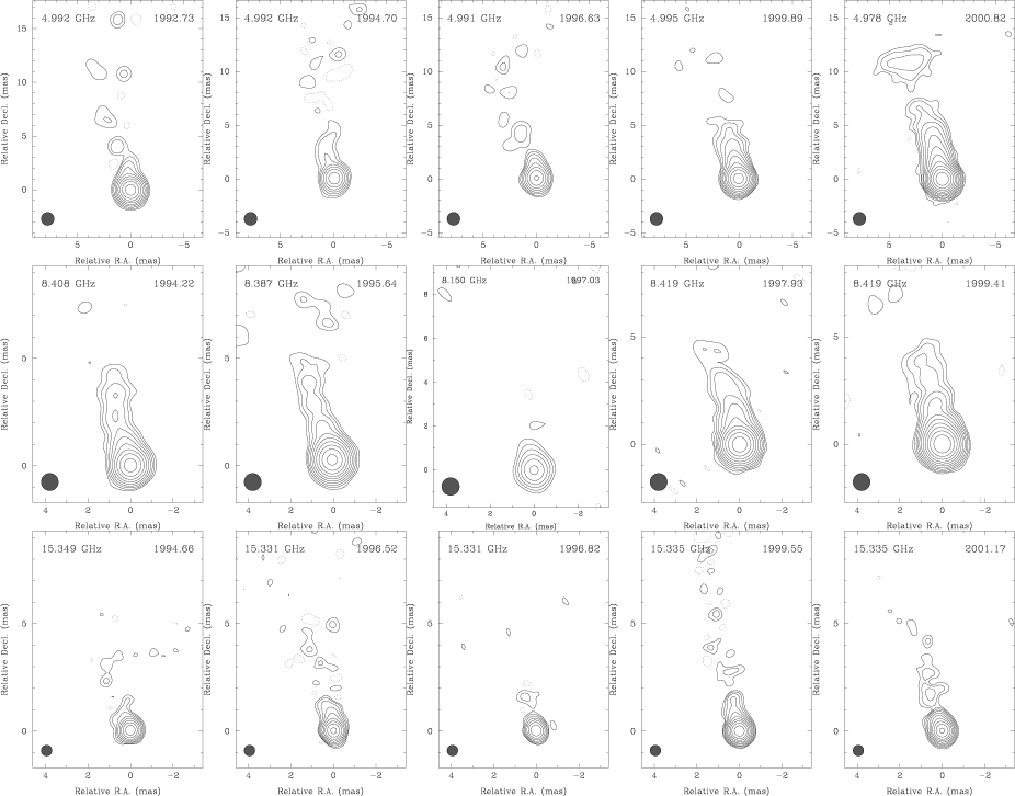
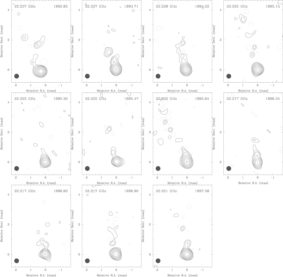
All data were correlated in the standard manner using the MK III correlator in Bonn and the VLBA correlator in Socorro. Part of the post-correlation analysis was done using NRAO’s Astronomical Image Processing System (Aips) and the Caltech VLBI Analysis Programs (Pearson & Readhead 1984). Data from other observers were provided as amplitude-calibrated and fringe fitted ($u,v$) FITS-files. The imaging of the source including phase and amplitude self-calibration was done using the CLEAN algorithm (Högbom 1974) and SELFCAL procedures in Difmap (Shepherd 1994). The self-calibration was done in steps of several phase-calibrations followed by careful amplitude calibration. During the iteration process the solution interval of the amplitude self-calibration was shortened from intervals as long as the whole observational time down to minutes. The resulting maps are presented in Figs. 1 & 2. Here, the jet is clearly visible to the north at P.A. $\sim 15\,^{\circ}$, and is slightly bent. At the lower frequencies we can follow the jet up to a distance of 10 mas to 15 mas from the core, whereas at the higher frequencies the jet is visible up to 3 mas.

Figure 1: All contour maps of 0716+714 at 5 GHz (top row), 8 GHz (middle) and 15 GHz (bottom). The maps are convolved with circular beams of 1.2 mas at 5 GHz, 0.8 mas at 8 GHz and 0.5 mas at 15 GHz. Total flux density, original beam size and the level of the lowest contour at three $\sigma$ are given in the observing log (Table 1). Contours are increasing by steps of two.

Figure 2: All contour maps of 0716+714 at 22 GHz. The maps are convolved with a circular beam of 0.3 mas. Total flux density, original beam size and the level of the lowest contour at three $\sigma$ are given in the observing log (Table 1). Contours are increasing by steps of two.

2.1 Model fits

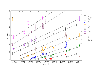
After imaging in Difmap we fitted circular Gaussian components to the self-calibrated data to parameterise the source structure seen in the VLBI maps. We used only circular components to reduce the number of free parameters and to simplify the analysis. A summary of the Gaussian component parameters from this model fitting is given in Table 2. For all model fits we used the brightest component as a reference and fixed its position to (0,0). The positions of the other components were measured relative to this component, which we assumed to be stationary (see Sect. 3.1 for details). A maximum uncertainty of 15 % in the flux density was estimated from the uncertainties of the amplitude calibration and from the formal errors of the model fits. The position error is given by $\Delta r=\frac{\sigma\cdot\Theta}{2S_{\rm P}}$ (Fomalont 1989), where $\sigma$ is the residual noise of the map after the subtraction of the model, $\theta$ the full width at half maximum (FWHM) of the component and $S_{\rm peak}$ the peak flux density. This formula tends to underestimate the error, if the peak flux density is very high or the width of the component is small. Therefore we included an additional error arising from the position variations during the model fitting procedure. In Fig. 3, the core distances of individual VLBI components derived from our model fits at various frequencies are plotted against time.

Figure 3: Core separation as a function of time for the individual modelfit components. Data from all frequencies are combined. Possible frequency-dependent position shifts are less than 0.1 mas and are not corrected. The solid lines show the linear fits to the path for each component. To show more clearly the well-defined components we do not show two of the farthest data points of C1 at $r=11.2$ mas and $r=11.9$ mas and one data point of C2 at $r=6.9$ mas.

3 Results and discussion

3.1 Identification of the components

To investigate the kinematics in the jet of 0716+714, we cross-identified individual model components along the jet using their distance from the VLBI core, flux density and size. Since the observations were not phase-referenced, the absolute position information was lost, and it is impossible to tell which components, if any, are stationary. To register the images and to test the stability of the VLBI-core position, we compared the core separations of the jet components of each epoch with respect to the adjacent observations, but we could not find any systematic position offsets. We also checked for position shifts between the jet components at higher and lower frequencies due to opacity effects (e.g., Lobanov 1998). Inspection of close or simultaneously observed frequency pairs does not show a systematic frequency shift between higher and lower frequencies larger than 0.1 mas (position accuracy between 15 GHz and 22 GHz is $<0.1$ mas). Therefore, we conclude that the core position is stationary and that all component positions can be measured with respect to this brightest component.

The cross identification of moving VLBI components between different times and frequencies is not unambiguous and depends on the dynamic range of the individual maps and on the time sampling. When we started our analysis we used the following scenarios as working hypotheses:

1. Stationary core with stationary or slow-moving jet,

2. Stationary core with fast moving jet,

3. Non-stationary core with fast or slow-moving jet,

4. Non-monotonic motion of the jet.

Figure 4: Core separation as a function of time for the components C5, C7, C8 and C9 separated for the different frequencies. The solid lines show the linear fits to the path for each component. Shifts between the paths at different frequencies are visible, but are typically smaller than the measured uncertainties.

As more data became available, we could rule out most of these identification schemes, and we were left with a scheme that assumes a stationary core and relatively fast component motion. The different schemes were tested, first separately at each frequency and later with all modelfits combined.

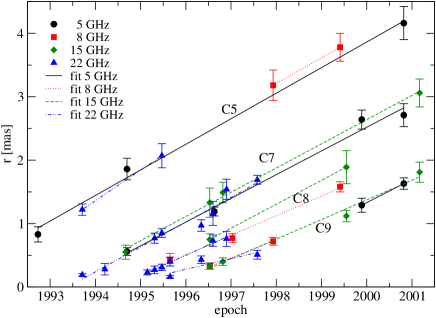
Supported by a graphical analysis, which is presented in Fig. 3, we could obtain a satisfactory scenario for the kinematics in the jet of 0716+714. This scenario consists of 11 identified superluminal components moving away from the core. As an example of the procedure used for all components we show the identification scheme for the separate frequencies for component C5, C7, C8 and C9 in Fig. 4. Again the frequency shifts between the trajectories are typically smaller than 0.1 mas to 0.2 mas and are smaller than the measurement uncertainty $\Delta r$.

Table 3 summarises the angular separation rate $\mu$ of the VLBI components derived from the linear fits of $r(t)$ and the corresponding apparent speed $\beta_{\rm app}=v_{\rm app}/c$ for an assumed redshift of 0.3.

3.2 The kinematic model

The components in this scenario move with 0.2 mas yr^-1 to 0.6 mas yr^-1 in the inner part of the VLBI jet ($r\leq 3$ mas) and with up to 0.9 mas yr^-1 in the outer regions. Due to the inhomogeneous time sampling, it is sometimes difficult to identify components over a long time interval. However, especially between 1993 and 1996, when we made many measurements spaced by only a few months, our proposed component identification gives the simplest and most reasonable fit to the data. Since most of our data were obtained at high frequencies, where the outer region of the jet is faint and already partly resolved by the interferometer beam, the parameter of the corresponding jet components (at $r\geq 4$ mas) are not as well constrained as the inner jet components and therefore they have larger positional errors. Despite this, there is still a very distinct tendency that the older components (C1 – C3), which now are located at large core separations, move faster than the components located in the inner jet (C4 – C10). This behaviour is also visible in Table 3, which shows a clear trend with systematically decreasing speeds between component C1 (16 $c$) and component C10 (4.5 $c$). The coarse time sampling for the individual jet components unfortunately does not allow us to fit acceleration to $r(t)$. Future and more densely sampled VLBI observations are required to show whether the inner jet components indeed move linearly.

Table 3: Proper motions in the jet of 0716+714. The number of data points which were used for the fit for each component is given in column 2. The last column gives the back-extrapolated ejection dates of the components, which result from the linear fits.

Id.	#	$\mu$ [mas/yr]	$\beta_{\rm app}\ (z=0.3)$	Ejection date
C1	4	$0.86\pm 0.13$	$16.13\,\pm\,2.36$	$1986.7\pm 1.3$
C2	5	$0.63\pm 0.10$	$11.87\,\pm\,1.82$	$1988.5\pm 1.0$
C3	8	$0.62\pm 0.04$	$11.59\,\pm\,0.76$	$1989.7\pm 0.3$
C4	7	$0.44\pm 0.01$	$8.27\,\pm\,0.24$	$1989.8\pm 0.1$
C5	7	$0.43\pm 0.02$	$8.16\,\pm\,0.29$	$1990.8\pm 0.2$
C6	9	$0.41\pm 0.02$	$7.80\,\pm\,0.33$	$1992.3\pm 0.1$
C7	17	$0.37\pm 0.01$	$6.89\,\pm\,0.19$	$1993.2\pm 0.1$
C8	11	$0.32\pm 0.01$	$6.04\,\pm\,0.20$	$1994.4\pm 0.1$
C9	10	$0.26\pm 0.01$	$4.98\,\pm\,0.27$	$1995.1\pm 0.1$
C10	3	$0.24\pm 0.01$	$4.52\,\pm\,0.45$	$1996.5\pm 0.2$
C11	2	$0.29\pm 0.02$	$5.48\,\pm\,0.55$	$1998.2\pm 0.3$

The luminosity distance $d_{\rm L}$ was calculated adopting the following relation

$$d_{\rm L}=\frac{c}{H_{0}}(1+z)\left[\eta(1,\Omega_{\rm m})-\eta(\frac{1}{1+z},\Omega_{\rm m})\right],$$ (1)

where

$$\eta(a,\Omega_{\rm m}) = 2\sqrt{s^{3}+1}\left[\frac{1}{a^{4}}-0.1540\frac{s}{a^{3}}+0.4304\frac{s^{2}}{a^{2}}\right.$$

$$\left.+0.19097\frac{s^{3}}{a}+0.066941s^{4}\right]^{-\frac{1}{8}},\quad{\rm with}$$

$$s^{3} = \frac{1-\Omega_{\rm m}}{\Omega_{\rm m}}\quad{\rm and}\quad a=\frac{1}{1+z},$$

which is an analytical fit (Pen 1999) to the luminosity distance for flat cosmologies with a cosmological constant. For the range of $0.2\leq\Omega_{\rm m}\leq 1.0$, the relative error of the distance is less than 0.4 % for any given redshift. Using

$$\beta_{\rm app}=\frac{\mu\ d_{\rm L}}{c\ (1+z)}$$ (2)

for the transformation of apparent angular separation rates ($\mu$) into spatial apparent speeds ($\beta_{\rm app}$) (Pearson & Zensus 1987) and assuming a redshift of 0.3 for 0716+714, one milliarcsecond corresponds to 4.4 pc. The measured angular separation rates then correspond to speeds of 4.5 $c$ to 16.1 $c$. For the components C3 to C9, for which the proper motion determination is the most confident (over seven data points), the average motion is $\mu=(0.41\pm 0.11)$ mas yr^-1 which corresponds to $\beta_{\rm app}=7.7\pm 2.1$. A preliminary analysis by Tian et al. (2001), who used only part of the data presented here, gave very similar speeds. A recently published kinematic analysis of the data from the VLBA 2 cm Survey also measured motion of 10 $c$ to 12 $c$ in the jet of 0716+714 (Kellermann et al. 2004). The speeds found in our paper are lower than the 16 $c$ to 21 $c$ found by Jorstad et al. (2001b), who observed the source over only a short time interval (3 yr). The difference between their and our results may be explained by slightly different (and unfortunately not unambiguous) map parameterisations using different Gaussian models or by non-linear component motion, with possible acceleration for shorter periods of time.

With an average apparent jet speed of about 8 $c$ and likely higher speeds of up to 15 $c$ to 20 $c$, 0716+714 displays considerably faster motion than other BL Lac objects, for which speeds of $\leq 5\,c$ are regarded as normal (e.g., Vermeulen & Cohen 1994; Gabuzda et al. 2000; Ros et al. 2002). In this context it appears that 0716+714 is an extreme BL Lac object with a jet speed (and Lorentz factor) much higher than regarded typical for BL Lac objects and close to the speeds of 10 $c$ to 20 $c$ seen in quasars.

3.3 Kinematics and geometry of the jet

Using the measured motion, $(11.6\pm 0.8)\,c$, of C3, the fastest, best-constrained jet component in our model, we can place limits on the jet speed and orientation of 0716+174. Adopting

$$\beta_{\rm app}=\frac{\beta\sin\theta}{1-\beta\cos\theta}$$ (3)

we find that the jet inclination that maximises the apparent speed, $\theta_{\rm max}$ is $4.9\,^{\circ}$. From that, one derives a minimum Lorentz factor, $\gamma_{\rm min}=(1+\beta_{\rm app}^{2})^{1/2}$ of $11.6$, which corresponds to a Doppler factor of $\delta_{\rm min}=\gamma_{\rm min}^{-1}(1-\beta_{\rm min}\cos\theta_{\rm max})^{-1}=11.7$, where $\beta_{\rm min}=\sqrt{1-\gamma_{\rm min}^{-2}}$. For smaller viewing angles ($\theta\rightarrow 0$) the Doppler factor approaches $\delta=2\gamma$, which yields $\delta=11.7$ to 23.4 at viewing angles between $4.9\,^{\circ}$ and $0\,^{\circ}$ for component C3. Including the higher values found by Jorstad et al. (2001b) and the highest speed derived from our data (16.1 $c$), a Doppler boosting factor of up to $\delta\geq 40$ appears possible.

Figure 5: The Doppler factor versus the apparent speed for constant intrinsic Lorentz factor, $\gamma$, (solid lines) and constant viewing angles $\theta$ (dotted lines). The range of measured speeds is indicated by the dashed lines and the grey shaded area marks the possible values for $\gamma$ and $\theta$ (see text for details).

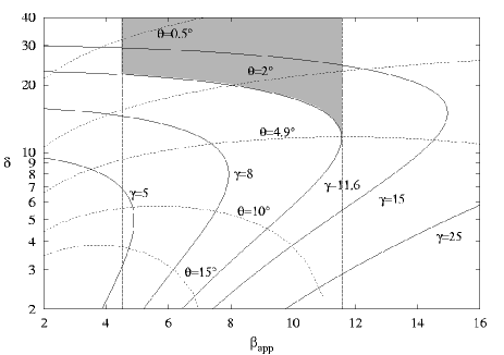
At cm-wavelengths, 0716+714 is a prominent intraday variable source, which shows amplitude variations of 5 % to 20 % on time-scales of 0.25 d to 2 d (Wagner et al. 1996; Kraus et al. 2003). Correlated radio-optical IDV observed in this source (Quirrenbach et al. 1991; Wagner et al. 1996; Qian et al. 1996) suggests that at least some fraction of the observed rapid variability has an intrinsic source origin and cannot be attributed to refractive interstellar scintillation (RISS) alone, as is done for some other IDV sources (e.g., Rickett 2001; Qian et al. 2001; Kedziora-Chudczer et al. 2001). The presence of the observed broad-band correlations of the variability and recently detected IDV at 9 mm wavelength, where RISS should not play a dominant role due to its $\lambda^{-2}$ dependence (cf. Krichbaum et al. 2002; Kraus et al. 2003), further support a non negligible intrinsic contribution to the IDV in 0716+714. In the following we use an average typical brightness temperature derived from the IDV observed at 6 cm of $10^{15.5}$ K to $10^{17}$ K. Slightly higher values of up to a few times $10^{18}$ K were measured only occasionally. To bring this brightness temperatures down to the inverse Compton limit of $10^{12}$ K, Doppler factors in the range of $\delta=(T_{\rm b}/10^{12}\,{\rm K})^{\frac{1}{3}}\approx 15$ to 50 are required. Adopting these Doppler factors, we obtain jet Lorentz factors of $\gamma\approx 8$ to 25 and viewing angles of $\theta\leq 1\,^{\circ}$.

The relation between the Doppler factor, intrinsic Lorentz factor, viewing angle and apparent speed is illustrated in Fig. 5. The Doppler factors derived from IDV lie within the grey shaded area.

If we now try to explain the observed range of apparent component speeds through variations of the viewing angle (under the assumption of a constant Lorentz factor along the jet), we cannot reach slow apparent speeds of $\sim 4.5$ $c$ without violating the lower limit of the Doppler factor of 2.1 from synchrotron self-Compton (SSC) models (Ghisellini et al. 1993). Therefore, we can exclude $\theta>5\,^{\circ}$ and the only solution remaining is to decrease the viewing angle which automatically leads to higher Doppler factors. The grey shaded area in Fig. 5 marks the allowed region of Lorentz factors and viewing angles. It becomes obvious that we need at least a Lorentz factor of $\gamma\approx 15$ and a viewing angle of the VLBI jet of $\theta\approx 2\,^{\circ}$ to explain the large range of observed apparent speeds as an effect of spatial jet bending. These values are consistent with those derived from IDV.

3.4 Flux density evolution

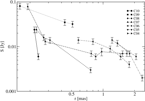
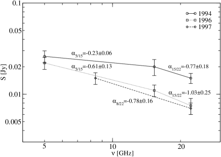
In Fig. 6 we show the evolution of the flux density of VLBI components at 22 GHz with their increasing separation from the core. We show this frequency because a large fraction of the data were obtained at 22 GHz (11 epochs). With the exception of a few data points, the components fade as they travel down the jet. This agrees qualitatively with the theory of a conically expanding jet (e.g., Blandford & Königl 1979). As the VLBI components expand they become optically thin and their spectra steepen. This is illustrated for component C7 in Fig. 7. The spectral index $\alpha$ is defined as $S\propto\nu^{\alpha}$. Knowing the turnover frequency and the size of a jet component allows us to calculate the strength of the magnetic field in the jet (e.g., Marscher 1983) as

$$B=10^{-5}\ b(\alpha)\ \frac{\theta^{4}\nu_{\rm m}^{5}\delta}{S_{\rm m}^{2}\,(1+z)}\ {\rm gauss},$$ (4)

where $b(\alpha)$ is a tabulated parameter dependent on the spectral index (Tab. 1 in Marscher 1983) with a value ranging from 1.8 to 3.8 for optically thin emission ($\alpha=-0.25$ to $-1.0$), $S_{\rm m}$ (in Jy) is the flux density at the turnover frequency $\nu_{\rm m}$ (in GHz) and $\theta$ (in mas) is the size of the component. If we calculate B for each of our modelfit components, without correcting for the Doppler factor $\delta$, we get the apparent magnetic field along the jet. Since we do not have adequate spectra for all positions along the jet we will consider a decrease of the turnover frequency along the jet proportional to $r^{p}$, to correct for the expansion of the component. The best results are obtained when we start with a turnover frequency of 4 GHz for the inner jet ($r\approx 0.2$ mas), that is plausible from the early spectrum (1994) of component C7 (Fig. 7) though the turnover is not actually observed, and use $p=-1.3$, which is in good agreement with the relativistic jet model (Marscher & Gear 1985). For all components along the jet we derive magnetic fields in the range of $10^{-4}\,\delta$ G to $10^{-7}\,\delta$ G. Since the minimum magnetic field strength that should be present due the energy density of the cosmic microwave background is a few microGauss (e.g., van der Laan & Perola 1969) the $10^{-7}\,\delta$ G already implies a lower limit of the Doppler factor of about 10. At this stage the core component is excluded from the analysis because both the source size and the turnover frequency are poorly known.

Figure 6: Flux density of the VLBI components at 22 GHz plotted versus core separation. The components fade as they travel down the jet.

Assuming equipartition between the energy of the particles, $E_{\rm e}$, and the energy of the magnetic field, $E_{\rm B}$, one can also derive the minimum magnetic field from the synchrotron luminosity, $L$.

$$L = 4\pi\ d_{\rm L}^{2}\ (1+z)\int_{\nu_{1}}^{\nu_{2}}\ S\ d\nu$$ (5)

$$E_{\rm e} = f(\alpha,\nu_{1},\nu_{2})\ L\ B^{-1.5},$$ (6)

where $f(\alpha,\nu_{1},\nu_{2})$ is a tabulated function (e.g. Pacholczyk 1970) and $\nu_{1}$ and $\nu_{2}$ are the upper and lower cutoff frequencies of the synchrotron spectrum with typically values of $10^{7}$ Hz to $10^{11}$ Hz. Taking the energy density of the magnetic field to be $1/8\pi\,B^{2}$ and assuming spherical symmetry the total energy of the source is

$$E_{\rm tot} = (1+k)E_{\rm e}+E_{\rm B}$$

$$= (1+k)\,f(\alpha,\nu_{1},\nu_{2})\ L\ B^{-1.5}+\frac{1}{6}\,R^{3}\,B^{2},$$

where $k$ is the energy ratio between the heavy particles and the electrons and $R$ is the size of the component. The ratio $k$ depends on the mechanism of generation of the relativistic electrons, which is unknown at the present. It can range from $k\approx 1$ for an electron-positron plasma up to $k\approx 2000$, if most of the energy is carried in the protons. We used $k\approx 100$ in our calculations, which seems to be a reasonable value (e.g., Pacholczyk 1970). Given that $E_{\rm e}\propto B^{-1.5}$ and $E_{\rm B}\propto B^{2}$, $E_{\rm tot}$ has a minimum and we find

$$B_{\rm min} = \left(\,\frac{9}{2}\,(1+k)\,f(\alpha,\nu_{1},\nu_{2})\ L\ R^{-3}\,\right)^{2/7}$$

$$= 5.37\cdot 10^{12}\ (S_{\rm m}\ \nu_{\rm m}\ d_{\rm L}^{2}\ R^{-3})^{2/7}.$$

with $k=100$, $f(-0.5,10^{7},10^{11})=1.6\cdot 10^{7}$ and $S_{\rm m}$ in Jy, $\nu_{\rm m}$ in GHz and $R$ in cm. Using $z=0.3$ and the same values for $S_{\rm m}$, $\nu_{\rm m}$ and $\theta$ as in Equation 4 we obtain magnetic fields between $10^{-4}$ G and $10^{-2}$ G for the jet. These values are larger than those derived before, which means that either the particle energy dominates and we do not have equipartition or that the emission is relativistically beamed. In the latter case, the different dependence of the magnetic field on the Doppler factor in Equation 4 ($B\propto\delta$) and in Equation 3.4 ($B_{\rm min}\propto\delta^{2/7\alpha+1}$) can be used to calculate the Doppler factor from $B_{\rm min}/B=\delta^{2/7\alpha}$. Comparing the results from all jet components yields Doppler factors of 4 to 15 with a mean value of 9. These values are slightly lower than those derived from the kinematics, but given that the calculations are based on many assumptions the values agree reasonably.

Figure 7: Spectral evolution of component C7.

In Fig. 8 we show the long-term radio variability and the spectral index of 0716+714 over the time range in which the VLBI components were born. We show a combined data set with flux density measurements at 5 GHz and 15 GHz from the UMRAO flux density monitoring program (Aller et al. 2003) and from our flux-density monitoring performed with the 100 m radio telescope at Effelsberg (Peng et al. 2000). A detailed discussion of the flux density variability using these and other data was recently done by Raiteri et al. (2003). Here, we restrict the discussion to a possible correlation of the radio variability with the ejection of new jet components. The ejection dates of new VLBI components are indicated by the grey shadowed areas. Their widths correspond to the uncertainty in the back-extrapolated ejection dates (see Table 3). Although these uncertainties are rather large and the time sampling of the light curves is not always dense enough, a weak correlation between the ejection of new components and the flares in the radio bands is obvious. Each of the shaded areas either lies at or shortly before the time of a flux density increase of at least one of the two observing bands.

Figure 8: The long term flux density variability of 0716+714 as measured at Effelsberg and with the Michigan radio telescope at 5 GHz (top) and 15 GHz (middle) and the spectral index (bottom), $\alpha_{5/15\,{\rm GHz}}$. The shaded areas mark the ejection dates of the VLBI components and their uncertainties.

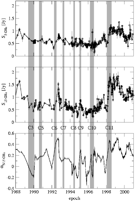
The two outbursts in mid 1992 and early 1995, which are best seen in the 2 cm band, are both surrounded by two new components, but the time sampling is too sparse to draw any further conclusions. In the lower panel of Fig. 8 we calculated the spectral index between 5 GHz and 15 GHz from the two light curves. Since the light curves were not measured simultaneously we searched for the closest pairs in the data set and calculated the spectral index from these pairs. The mean separation between two points is about eight days. The graph itself represents an eight-point running average to reduce the noise in the data. This figure shows an obvious correlation between the spectral index variations and the ejection of a new VLBI component. Seven out of eight ejections (except C9) of new VLBI components are accompanied by a flattening of the source spectrum. The flattening is in good agreement with an expanding component that becomes optically thin first at the higher frequency and later at the lower frequency (e.g., Marscher & Gear 1985).

We note that at the times of particularly dense time sampling (after 1994) a number of minor radio flares are visible, which are not related to the ejection of any of the known VLBI components. According to the light-house model and other related helical jet models (e.g., Camenzind & Krockenberger 1992; Roland et al. 1994) it is possible that initial outbursts, which are related to the ejection of new jet components are followed by secondary flux density variations, which are not or only are indirectly related to the component ejection. Of course, it is also possible that we missed some jet components in our infrequently sampled VLBI monitoring.

To test the significance of the correlations found by eye, we placed eight fields with a similar width randomly over the light curves between 1989 and 1999 and determined how many are coincident with a flare in the light curve or a flattening of the spectrum. For the light curves this test yielded a 50 % probability of our results occurring at random. The probability of measuring a flattening of the spectrum in seven out of eight components selected at random from our spectrum is 5.7 %. Generally a result is excepted to be statically significant if the probability is below 5 %, which means that the correlations of the light curve with the ejection dates are likely to be a coincidence, but given that we might have missed a component the correlation of the spectral index is more significant. A coordinated and much denser sampled multi-frequency flux density and VLBI monitoring is necessary to study in more detail such outburst-ejection relations.

3.5 Connection with $\gamma$-ray flares

0716+714 was detected at $\gamma$-rays by the EGRET detector on board the Compton Gamma Ray Observatory (Hartman et al. 1999; Mattox et al. 1997). Since it is proposed that the $\gamma$-ray emission, like the radio emission, is Doppler boosted (Dermer & Schlickeiser 1994), the $\gamma$-ray detection of 0716+714 yields further evidence for a high Lorentz factor in the jet.

Recent studies about the connection between $\gamma$-ray sources and superluminal VLBI-components suggest that these sources have higher average jet speeds than sources which are not detected at $\gamma$-rays (Jorstad et al. 2001a; Kellermann et al. 2004). Moreover, Jorstad et al. (2001a) found a correlation between the ejection of new VLBI components and the appearance of $\gamma$-ray flares, suggesting that the radio and the $\gamma$-ray emission originate within the same shocked area in the relativistic jet. The authors report a $\gamma$-ray flare of 0716+714 in 1992.2 which appears to be coincident with a peak in the linear polarization light-curve at 15 GHz. Unfortunately, their 0716+714 VLBI data does not cover this period, but with our larger sample we found a new VLBI component (C6) with an extrapolated ejection date of $1992.3\pm 0.1$ which is in good agreement with the reported $\gamma$-ray flare. Although we register three additional ejections up to 1996 and 0716+714 was observed several times by EGRET in this period, no more flares were detected. But given that the $\gamma$-ray measurements have large uncertainties and only 18 data points were recorded during these four years, this seems not exceptional. Similar outburst ejection events were also found in e.g, 0528+134 (Krichbaum et al. 1995) and 0836+710 (Otterbein et al. 1998). Assuming that the correlation between the new component, C6, and the 1992.2 flare is real, this supports the idea that the $\gamma$-ray emission originates from the same region from which we observe the radio emission (e.g., Sikora et al. (1994)).

3.6 Variation of the ejection position angle and core flux density

The visual inspection of position angle of the innermost portion of the VLBI jet in the maps of Figs. 1 & 2 indicates a variation of the P.A. of the jet near the core with time. In order to quantify this, we used the Gaussian models and fitted a straight line to the first milliarcsecond of the jet. For each observing epoch, the position angle of this line provides a good estimate of the direction of the inner portion of the VLBI jet. In Fig. 9 (top panel) we plot the P.A. grouped in one year time bins.

Figure 9: Top: Position angle of the central 1 mas of the VLBI jet grouped in one year time bins. The dashed line is a sinusoidal fit to the data. The position angle of the inner jet (ejection angle) varies with a period of $\sim 7.4$ years. Bottom: One year bins of the 22 GHz core flux density. The dashed line represents a sinusoidal fit with a fixed period of 7.4 years.

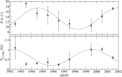
A sinusoidal fit to the data reveals a period of ($7.4\pm 1.5$) yr. The fit yields a reduced $\chi_{\rm r}^{2}$ of 1.55, which is much better than the $\chi_{\rm r}^{2}$ of 4.28, obtained for a linear fit. Unfortunately our data cover only one period of the variability and it will be interesting to see if the trend holds in the future. A possible explanation for such periodic variation would be a precessing footpoint of the jet. This should also result in a flux density variation of the VLBI core, and indeed, there is a tendency that the core flux density at 22 GHz is consistent with a periodic variation of $\sim 7$ yr (see Fig. 9, bottom panel). Recently Raiteri et al. (2003) published an analysis of the optical and radio flux density variability of 0716+714 and found a periodicity of 5.5 yr to 6.0 yr for the flux-density variations in the radio regime. This is compatible within the error bars with the periodicity of the P.A. in the inner region of the jet. Based on the geometrical considerations in Sect. 3.3, the apparent peak to peak variation of $\approx 7\,^{\circ}$ of the ejection angle corresponds to a small change of only $7\,^{\circ}\sin\theta\approx 0.6\,^{\circ}$ of the jet direction.

Such small variations of a few degrees in the rest frame of the source in several years have recently been detected also in other AGN, e.g. 3C 345 (Biretta et al. 1986), 3C 279 (Carrara et al. 1993), 3C 273 (Krichbaum et al. 2001) and BL Lac (Stirling et al. 2003). The most common explanation is a precessing jet, which could be caused by a binary super-massive black hole system (Biretta et al. 1986; Hummel et al. 1992) or a warped accretion disc (Lai 2003 and ref. therein). However, hydrodynamic effects also can lead to a precession of the jet (e.g., Hughes et al. 2002). In this case the precession is introduced by a potentially strong oblique internal shock that arises from asymmetric perturbation of the flow.

3.7 Redshift dependence of the results

Since all the derived parameters of the kinematics and geometry scale with the distance to 0716+714, knowing the redshift is of great importance. The distance to 0716+714 and therewith the speeds of the jet components scale nearly linearly with $z$ at these low redshifts. Thus a redshift decrease by a factor of three would also decrease the Doppler factor by three. The dependence of brightness temperature derived from IDV is $T_{\rm b}\propto\left(\frac{z}{1+z}\right)^{2}$ (e.g., a decrease from $z=0.3$ to $z=0.1$ would reduce $T_{\rm b}$ by 6.4). Since, $T_{\rm b}\propto\delta^{3}$ this would increase the discrepancy between the Doppler factor, which is needed to reduce $T_{\rm b}$ and the Doppler factor derived from the kinematics. An increase in redshift would bring the derived parameters closer together.

Our assumption of the redshift of $z\geq 0.3$ is based on the non-detection of an underlying host galaxy by Wagner et al. (1996). BL Lac host galaxies have typical absolute magnitudes of $M_{\rm R}\approx-24$ and an effective radius of $r_{\rm c}\approx 10$ kpc (Jannuzi et al. 1997 and ref. therein). The lower limit of Wagner et al. corresponds to an absolute magnitude of $M_{\rm R}=-20.4$, which would be an unusually faint BL Lac host and so is a very conservative lower limit. An upper limit for the redshift can be given from the lack of absorption by foreground galaxies, which results in a redshift of $z\leq 0.5$ (Wagner priv. comm.). At present it is unclear if the tentative X-ray detection of a spectral line near 5.8 keV (Kadler et al. 2004) can be identified with the Fe K_α line. If so, the redshift of the line would indicate a distance of $z=0.10\pm 0.04$, much closer than expected from the optical measurements. Possible ways out of this difficulty could invoke a blue shift of the line or some external emission process not related to the nucleus of 0716+71. A solid confirmation of the X-ray line in future observations is urgently needed.

4 Conclusions

We analysed 26 epochs of VLBI data at 4.9 GHz, 8.4 GHz, 15.3 GHz, and 22.2 GHz observed over 10 yr, between 1992 and 2001, and derived a new kinematic scenario for the jet in 0716+714. In this scenario the components move with apparent speeds of 4.5 $c$ to 16.1 $c$ ($z=0.3$). These speeds are atypically fast for BL Lac objects, which typically exhibit speeds of $\leq 5\,c$ (e.g., Vermeulen & Cohen 1994; Gabuzda et al. 2000; Ros et al. 2002). Since this analysis is based on much denser sampled VLBI data than previous studies, we are convinced that we can rule out the somewhat slower scenarios which were presented previously (e.g., Witzel et al. 1988; Schalinski et al. 1992; Gabuzda et al. 1998). We find a periodic variation of the P.A. of the innermost jet which could be a sign of jet precession on a time-scale of ($7.4\pm 1.5$) yr. If this can be confirmed in future observations the higher speeds found by Jorstad et al. (2001b) might be explained by non-linear motion of the jet components.

No correlation was found between the component ejection and radio flux density flares at the cm-wavelengths. There seems to be a weak correlation between the ejection of new components and the flattening of the radio spectrum. For one of the new components (C6) we could find a reported $\gamma$-ray flare and if the ejection and the flare are really connected this would support the idea that the $\gamma$-ray emission originates from the same region from which we observe the radio emission.

From the component motion in the jet, we obtain a lower limit for the Lorentz factor of 11.6 and a maximum angle to the line of sight of $4.9\,^{\circ}$. To explain the large range of observed apparent speeds as an effect of spatial jet bending, a Lorentz factor of $\gamma>15$ and a viewing angle of the VLBI jet of $\theta<2\,^{\circ}$ are more likely. Under these circumstances, the Doppler factor would be $\delta\approx 20$ to 30. Such high Doppler factors are indeed required to explain the high apparent brightness temperatures of up to $10^{17}$ K derived from intraday variability at cm-wavelengths.

Table 2: Results from Gaussian Model fitting and component parameters. $S_{\rm peak}$ is the peak flux density, $r$ and $\phi$ are the distance and the P.A. measured from the core and $\theta$ is the FWHM of the Gaussian component.

Epoch	$\nu$	$S_{\rm peak}$	$r$	$\phi$	$\theta$	Id.a
	[GHz]	$[\frac{mJy}{beam}]$	[mas]	[∘]	[mas]
1992.73	$5.0$	$596\,\pm\,89.4$	–	–	$0.10\,\pm\,0.02$	Core
		$37\,\pm\,5.5$	$0.83\,\pm\,0.12$	$17\,\pm\,8$	$0.14\,\pm\,0.03$	C5
		$19\,\pm\,2.8$	$1.92\,\pm\,0.13$	$8\,\pm\,3$	$0.60\,\pm\,0.12$	C3
		$8\,\pm\,1.2$	$5.02\,\pm\,0.24$	$17\,\pm\,2$	$0.93\,\pm\,0.19$	C1
		$7\,\pm\,1.0$	$11.46\,\pm\,0.49$	$13\,\pm\,2$	$3.35\,\pm\,0.67$	X
1992.85	$22.2$	$708\,\pm\,106.2$	–	–	$0.18\,\pm\,0.04$	Core
		$12\,\pm\,1.8$	$1.37\,\pm\,0.06$	$12\,\pm\,2$	$0.10\,\pm\,0.02$	C4
		$16\,\pm\,2.4$	$2.86\,\pm\,0.22$	$0\,\pm\,4$	$1.48\,\pm\,0.30$	C2
1993.71	$22.2$	$272\,\pm\,40.8$	–	–	$0.05\,\pm\,0.01$	Core
		$79\,\pm\,11.8$	$0.19\,\pm\,0.02$	$15\,\pm\,5$	$0.05\,\pm\,0.01$	C7
		$14\,\pm\,2.1$	$0.58\,\pm\,0.07$	$14\,\pm\,6$	$0.12\,\pm\,0.02$	C6
		$14\,\pm\,2.1$	$1.22\,\pm\,0.09$	$20\,\pm\,4$	$0.23\,\pm\,0.05$	C5
1994.21	$22.2$	$309\,\pm\,46.3$	–	–	$0.09\,\pm\,0.02$	Core
		$15\,\pm\,1.9$	$0.28\,\pm\,0.09$	$28\,\pm\,18$	$0.01\,\pm\,0.00$	C7
		$13\,\pm\,1.9$	$0.80\,\pm\,0.13$	$15\,\pm\,9$	$0.42\,\pm\,0.08$	C6
		$7\,\pm\,1.0$	$1.79\,\pm\,0.16$	$14\,\pm\,5$	$0.38\,\pm\,0.08$	C4
1994.21	$8.4$	$266\,\pm\,39.9$	–	–	$0.14\,\pm\,0.03$	Core
		$25\,\pm\,3.7$	$0.82\,\pm\,0.09$	$13\,\pm\,6$	$0.42\,\pm\,0.08$	C6
		$10\,\pm\,1.5$	$1.99\,\pm\,0.19$	$17\,\pm\,5$	$0.76\,\pm\,0.15$	C4
		$9\,\pm\,1.3$	$3.27\,\pm\,0.22$	$12\,\pm\,3$	$0.84\,\pm\,0.17$	C2
		$4\,\pm\,0.6$	$4.70\,\pm\,0.43$	$14\,\pm\,5$	$1.48\,\pm\,0.30$	X
1994.67	$15.3$	$413\,\pm\,61.9$	–	–	$0.07\,\pm\,0.01$	Core
		$20\,\pm\,4.0$	$0.55\,\pm\,0.11$	$14\,\pm\,11$	$0.64\,\pm\,0.13$	C7
		$14\,\pm\,2.1$	$2.82\,\pm\,0.24$	$14\,\pm\,5$	$1.68\,\pm\,0.34$	C3
1994.70	$5.0$	$284\,\pm\,42.6$	–	–	$0.18\,\pm\,0.04$	Core
		$26\,\pm\,3.9$	$0.56\,\pm\,0.06$	$7\,\pm\,6$	$0.21\,\pm\,0.04$	C7
		$13\,\pm\,1.9$	$1.86\,\pm\,0.17$	$18\,\pm\,5$	$0.77\,\pm\,0.15$	C5
		$12\,\pm\,1.8$	$3.00\,\pm\,0.17$	$15\,\pm\,3$	$0.72\,\pm\,0.14$	C3
		$7\,\pm\,1.0$	$4.34\,\pm\,0.32$	$8\,\pm\,4$	$1.45\,\pm\,0.29$	C2
1995.15	$22.2$	$724\,\pm\,108.6$	–	–	$0.07\,\pm\,0.01$	Core
		$24\,\pm\,3.6$	$0.23\,\pm\,0.04$	$12\,\pm\,9$	$0.07\,\pm\,0.01$	C8
		$9\,\pm\,1.3$	$1.17\,\pm\,0.06$	$12\,\pm\,3$	$0.07\,\pm\,0.01$	C6
		$2\,\pm\,0.3$	$2.37\,\pm\,0.19$	$14\,\pm\,4$	$0.15\,\pm\,0.03$	C4
		$10\,\pm\,1.5$	$3.43\,\pm\,0.10$	$15\,\pm\,1$	$0.20\,\pm\,0.04$	C3
1995.31	$22.2$	$421\,\pm\,63.1$	–	–	$0.10\,\pm\,0.02$	Core
		$16\,\pm\,2.4$	$0.27\,\pm\,0.06$	$12\,\pm\,11$	$0.10\,\pm\,0.02$	C8
		$7\,\pm\,1.0$	$0.77\,\pm\,0.08$	$14\,\pm\,6$	$0.10\,\pm\,0.02$	C7
1995.47	$22.2$	$174\,\pm\,26.1$	–	–	$0.04\,\pm\,0.01$	Core
		$14\,\pm\,2.1$	$0.31\,\pm\,0.05$	$29\,\pm\,9$	$0.07\,\pm\,0.01$	C8
		$6\,\pm\,0.9$	$0.85\,\pm\,0.07$	$18\,\pm\,4$	$0.06\,\pm\,0.01$	C7
		$6\,\pm\,0.9$	$2.07\,\pm\,0.19$	$23\,\pm\,5$	$0.43\,\pm\,0.09$	C5
1995.65	$22.2$	$220\,\pm\,33.0$	–	–	$0.07\,\pm\,0.01$	Core
		$81\,\pm\,12.1$	$0.16\,\pm\,0.02$	$10\,\pm\,6$	$0.05\,\pm\,0.01$	C9
		$29\,\pm\,4.3$	$0.40\,\pm\,0.07$	$13\,\pm\,10$	$0.32\,\pm\,0.06$	C8
1995.65	$8.4$	$252\,\pm\,37.8$	–	–	$0.11\,\pm\,0.02$	Core
		$32\,\pm\,4.8$	$0.43\,\pm\,0.10$	$9\,\pm\,12$	$0.10\,\pm\,0.02$	C8
		$8\,\pm\,1.2$	$1.36\,\pm\,0.18$	$15\,\pm\,7$	$0.53\,\pm\,0.11$	C6
		$3\,\pm\,0.4$	$2.64\,\pm\,0.26$	$20\,\pm\,5$	$0.40\,\pm\,0.08$	C4
		$5\,\pm\,0.8$	$3.97\,\pm\,0.34$	$15\,\pm\,5$	$1.19\,\pm\,0.24$	C3
1996.34	$22.2$	$221\,\pm\,33.1$	–	–	$0.08\,\pm\,0.02$	Core
		$35\,\pm\,5.3$	$0.43\,\pm\,0.06$	$9\,\pm\,7$	$0.24\,\pm\,0.05$	C9
		$10\,\pm\,1.5$	$0.97\,\pm\,0.09$	$12\,\pm\,5$	$0.15\,\pm\,0.03$	C7
		$6\,\pm\,0.9$	$1.47\,\pm\,0.13$	$5\,\pm\,5$	$0.20\,\pm\,0.04$	C6
1996.53	$15.3$	$225\,\pm\,33.8$	–	–	$0.08\,\pm\,0.02$	Core
		$17\,\pm\,2.6$	$0.33\,\pm\,0.05$	$9\,\pm\,8$	$0.08\,\pm\,0.02$	C9
		$15\,\pm\,2.2$	$0.75\,\pm\,0.09$	$4\,\pm\,6$	$0.23\,\pm\,0.05$	C8
		$4\,\pm\,0.6$	$1.33\,\pm\,0.23$	$17\,\pm\,9$	$0.43\,\pm\,0.09$	C7
		$3\,\pm\,0.4$	$4.12\,\pm\,0.34$	$15\,\pm\,4$	$0.71\,\pm\,0.14$	C3
		$1\,\pm\,0.1$	$5.14\,\pm\,0.24$	$27\,\pm\,2$	$0.12\,\pm\,0.02$	C2
1996.60	$22.2$	$218\,\pm\,32.7$	–	–	$0.06\,\pm\,0.01$	Core
		$17\,\pm\,2.6$	$0.73\,\pm\,0.09$	$6\,\pm\,6$	$0.26\,\pm\,0.05$	C8
		$3\,\pm\,0.4$	$1.16\,\pm\,0.19$	$15\,\pm\,9$	$0.22\,\pm\,0.04$	C7
		$4\,\pm\,0.6$	$1.78\,\pm\,0.08$	$19\,\pm\,2$	$0.05\,\pm\,0.01$	C6
1996.63	$5.0$	$183\,\pm\,27.4$	–	–	$0.03\,\pm\,0.01$	Core
		$22\,\pm\,3.3$	$1.19\,\pm\,0.07$	$9\,\pm\,3$	$0.24\,\pm\,0.05$	C7
		$8\,\pm\,1.2$	$4.09\,\pm\,0.27$	$20\,\pm\,3$	$1.19\,\pm\,0.24$	C3
		$7\,\pm\,1.0$	$9.58\,\pm\,0.49$	$23\,\pm\,2$	$3.39\,\pm\,0.68$	C1
		$3\,\pm\,0.4$	$12.06\,\pm\,0.44$	$10\,\pm\,2$	$1.14\,\pm\,0.23$	X
1996.82	$15.3$	$251\,\pm\,37.6$	–	–	$0.01\,\pm\,0.00$	Core
		$13\,\pm\,1.9$	$0.40\,\pm\,0.06$	$19\,\pm\,7$	$0.08\,\pm\,0.02$	C9
		$10\,\pm\,1.5$	$1.49\,\pm\,0.16$	$12\,\pm\,6$	$0.51\,\pm\,0.10$	C7
1996.90	$22.2$	$260\,\pm\,39.0$	–	–	$0.04\,\pm\,0.01$	Core
		$24\,\pm\,3.6$	$0.22\,\pm\,0.04$	$22\,\pm\,10$	$0.08\,\pm\,0.02$	C10
		$3\,\pm\,0.4$	$0.76\,\pm\,0.12$	$16\,\pm\,8$	$0.08\,\pm\,0.02$	C8
		$7\,\pm\,1.0$	$1.54\,\pm\,0.16$	$7\,\pm\,6$	$0.38\,\pm\,0.08$	C7
		$3\,\pm\,0.4$	$4.69\,\pm\,0.29$	$13\,\pm\,3$	$0.50\,\pm\,0.10$	C3
continued on next Col.

Table 2: Modelfit parameters (continued from previous Col.).

Epoch	$\nu$	$S_{\rm peak}$	$r$	$\phi$	$\theta$	Id.
	[GHz]	$[\frac{mJy}{beam}]$	[mas]	[∘]	[mas]
1997.03	$8.4$	$194\,\pm\,29.2$	–	–	$0.09\,\pm\,0.02$	Core
		$22\,\pm\,3.3$	$0.77\,\pm\,0.07$	$12\,\pm\,5$	$0.23\,\pm\,0.05$	C8
1997.58	$22.2$	$929\,\pm\,139.4$	–	–	$0.07\,\pm\,0.01$	Core
		$6\,\pm\,0.9$	$0.24\,\pm\,0.14$	$43\,\pm\,29$	$0.01\,\pm\,0.00$	C10
		$32\,\pm\,4.8$	$0.51\,\pm\,0.07$	$7\,\pm\,7$	$0.32\,\pm\,0.06$	C9
		$7\,\pm\,1.0$	$1.69\,\pm\,0.07$	$11\,\pm\,2$	$0.06\,\pm\,0.01$	C7
1997.93	$8.4$	$385\,\pm\,57.7$	–	–	$0.10\,\pm\,0.02$	Core
		$19\,\pm\,2.8$	$0.72\,\pm\,0.06$	$14\,\pm\,5$	$0.16\,\pm\,0.03$	C9
		$15\,\pm\,2.2$	$1.54\,\pm\,0.10$	$7\,\pm\,3$	$0.30\,\pm\,0.06$	C7
		$7\,\pm\,1.0$	$3.18\,\pm\,0.24$	$15\,\pm\,4$	$0.84\,\pm\,0.17$	C5
1999.41	$8.4$	$922\,\pm\,138.3$	–	–	$0.10\,\pm\,0.02$	Core
		$60\,\pm\,9.0$	$0.68\,\pm\,0.07$	$10\,\pm\,5$	$0.10\,\pm\,0.02$	C10
		$17\,\pm\,2.6$	$1.58\,\pm\,0.08$	$13\,\pm\,2$	$0.20\,\pm\,0.04$	C8
		$4\,\pm\,0.6$	$3.16\,\pm\,0.19$	$6\,\pm\,3$	$0.28\,\pm\,0.06$	C6
		$4\,\pm\,0.6$	$3.78\,\pm\,0.22$	$15\,\pm\,3$	$0.40\,\pm\,0.08$	C5
1999.55	$15.3$	$1157\,\pm\,173.6$	–	–	$0.06\,\pm\,0.01$	Core
		$54\,\pm\,8.1$	$0.40\,\pm\,0.03$	$15\,\pm\,3$	$0.08\,\pm\,0.02$	C11
		$26\,\pm\,3.9$	$1.12\,\pm\,0.09$	$12\,\pm\,4$	$0.39\,\pm\,0.08$	C9
		$2\,\pm\,0.3$	$1.89\,\pm\,0.26$	$10\,\pm\,8$	$0.28\,\pm\,0.06$	C8
		$10\,\pm\,1.5$	$2.90\,\pm\,0.24$	$9\,\pm\,4$	$1.17\,\pm\,0.23$	C6
1999.89	$5.0$	$558\,\pm\,83.7$	–	–	$0.18\,\pm\,0.04$	Core
		$39\,\pm\,5.9$	$1.29\,\pm\,0.11$	$8\,\pm\,5$	$0.13\,\pm\,0.03$	C9
		$19\,\pm\,2.8$	$2.64\,\pm\,0.15$	$10\,\pm\,3$	$0.83\,\pm\,0.17$	C7
		$6\,\pm\,0.9$	$4.43\,\pm\,0.29$	$12\,\pm\,3$	$1.00\,\pm\,0.20$	C4
		$1\,\pm\,0.1$	$6.92\,\pm\,0.98$	$18\,\pm\,8$	$1.93\,\pm\,0.39$	C2
		$7\,\pm\,1.0$	$11.86\,\pm\,0.58$	$17\,\pm\,2$	$4.79\,\pm\,0.96$	C1
2000.82	$5.0$	$520\,\pm\,78.1$	–	–	$0.12\,\pm\,0.02$	Core
		$35\,\pm\,5.3$	$0.77\,\pm\,0.12$	$20\,\pm\,8$	$0.10\,\pm\,0.02$	C11
		$25\,\pm\,3.9$	$1.63\,\pm\,0.09$	$12\,\pm\,3$	$0.42\,\pm\,0.08$	C9
		$11\,\pm\,1.6$	$2.71\,\pm\,0.18$	$11\,\pm\,3$	$0.74\,\pm\,0.15$	C7
		$9\,\pm\,1.4$	$4.16\,\pm\,0.26$	$11\,\pm\,3$	$1.25\,\pm\,0.25$	C5
		$8\,\pm\,1.3$	$11.16\,\pm\,0.51$	$17\,\pm\,2$	$4.43\,\pm\,0.89$	C1
2001.17	$15.3$	$549\,\pm\,82.4$	–	–	$0.06\,\pm\,0.01$	Core
		$72\,\pm\,10.8$	$0.45\,\pm\,0.04$	$20\,\pm\,4$	$0.18\,\pm\,0.04$	C12
		$14\,\pm\,2.1$	$1.81\,\pm\,0.16$	$17\,\pm\,5$	$0.70\,\pm\,0.14$	C9
		$5\,\pm\,0.8$	$3.06\,\pm\,0.22$	$13\,\pm\,4$	$0.49\,\pm\,0.10$	C7
		$3\,\pm\,0.4$	$5.08\,\pm\,0.29$	$16\,\pm\,3$	$0.51\,\pm\,0.10$	C4