Correlation between the TeV and X–ray emission in high–energy peaked BL Lac objects.

We discuss the correlation between the evolution of the TeV emission and X–ray radiation observed in high-energy peaked BL Lac objects. We describe such a correlation by a simple power law $F_{\rm TeV}(t)\propto F^{x}_{\rm X-ray}(t)$. In the first part of this work we present correlations obtained for the activity of Mrk 501 observed in 1997 April and for the activity of Mrk 421 observed in 2000 February. Our results obtained for Mrk 501 show that the index of the correlation ($x$) may strongly depend on the width and position of the spectral bands used for the comparison. The result of the correlation which we have obtained for Mrk 421 is not informative. However, we discuss results of similar correlation obtained for this source by other authors. They report an almost quadratic ($x\sim 2$) correlations observed between the evolution of the TeV and X–ray emission. In the second part of this paper we present a phenomenological model which describes the evolution of the synchrotron and inverse Compton emission of a simple spherical homogeneous source. Neglecting the radiative cooling of the particles we derive analytical expressions that describe the evolution. Then we use a numerical code to investigate the impact of radiative cooling on the evolution. We show that different forms of correlations can be obtained depending on the assumed evolution scenario and the spectral bands used for the calculation. However, the quadratic correlation observed during the decay phase of the flare observed in Mrk 421 on 2001 March 19 appears problematic for this basic modeling. The quadratic correlation can be explained only for specific choices of the spectral bands used for the calculation. Therefore, looking for more robust solutions, we investigate the evolution of the emission generated by a cylindrical source. However this model does not provide robust solutions for the problem of a quadratic correlation. In principle the problem could be solved by the TeV emission generated by the self Compton scattering in the Thomson limit. However, we show that such a process requires unacceptably large values of the Doppler factor. Finally we briefly discuss the possible influence of the light travel time effect on our results.

1 Introduction

The emission from BL Lacertae objects is dominated by the intense relativistic boosted non–thermal continuum produced within a relativistic jet closely aligned with the line of sight, making these objects (together with Flat Spectrum Radio Quasars, the other subgroup of the blazars family) the best laboratories to study the physics of relativistic jets.

The overall emission, from radio to $\gamma$–rays (extended in some cases to the multi–TeV band), shows the presence of two well–defined broad components, the first one peaking in the optical–soft-X–ray bands, the second one in the GeV–TeV region. The low energy peak is attributed to synchrotron emission by relativistic electrons in the jet, while the second component is commonly believed to be Inverse Compton emission (hereafter IC) from the same electron population (although different scenarios have been proposed, see e.g. Mannheim mannheim93 (1993), Aharonian aharonian00 (2000), Pohl & Schlickeiser pohl00 (2000), Mucke et al. mucke03 (2003)).

BL Lacs are further subdivided in Low–energy Peak BL Lacs (LBL), exhibiting the synchrotron peak in the IR-optical region of the spectrum, and High–energy Peak BL Lacs (HBL), in which the synchrotron peak can lie in the UV–X–ray band. The almost featureless optical spectra of HBL clearly indicate that the environment external to the jet is quite poor in soft photons, suggesting that the high–energy emission is mainly produced through the Comptonization of the synchrotron radiation (Synchrotron Self–Compton emission, SSC). The few extragalactic TeV sources firmly detected so far (Mrk 421, Mrk 501, PKS 2344+514, PKS 2155–304, 1ES1959+65, 1ES 1426+428, e.g. Krawczynski krawczynski04 (2004) for a recent review) belong to this class.

Since the discovery of the first BL Lac object emitting TeV radiation, Mrk 421, (Punch et al. punch92 (1992)) TeV blazars have been the target of very intense observational and theoretical investigations. Indeed the possibility of observing the emission produced by very high energy electrons (up to Lorentz factors of the order of $10^{7}$) coupled with observations in the X–ray band, where the synchrotron peak of these sources is usually located, offers a unique tool to probe the processes responsible for the cooling and the acceleration of relativistic particles.

Studies conducted simultaneously in the X–ray and in the TeV bands are of particular importance, since in the simple SSC framework one expects that variations in X–rays and TeV should be closely correlated, being produced by electrons with similar energies. Assuming a typical magnetic field intensity $B\sim 0.1$ G and Doppler factor $\delta\sim 10$, photons with energy E $\sim 1$ keV are emitted by electrons with Lorentz factor $\gamma\sim 10^{6}$. The same electrons will upscatter photons at energy $E\sim\gamma mc^{2}\sim 1$ TeV (since the Lorentz factor is extremely large the scattering will occur in the Klein–Nishina regime even with optical target photons). In fact observations at X–ray and TeV energies (Buckley et al. buckley96 (1996), Catanese et al. catanese97 (1997)) yielded significant evidence of correlated and simultaneous variability of the TeV and X–ray fluxes. During the X/TeV 1998 campaign on Mrk 421 a flare was detected simultaneously both at X–ray and TeV energies and the maxima were simultaneous within 1 hour, confirming that variations in these two bands are closely related (Maraschi et al. maraschi99 (1999)). Subsequent more extensive analyses confirmed these first results also in other sources. Note however that the correlation seems to be violated in some cases, as indicated by the observation of an “orphan” (i.e. not accompanied by the corresponding X–ray flare) TeV event in the BL Lac 1ES 1959+650 (Krawczynski et al. krawczynski04a (2004)).

Although the study of TeV BL Lacs has been the subject of great effort in the past (e.g. Böttcher bottcher04 (2004), Georganopoulos & Kazanas georg03 (2003), Moderski, Sikora & Blazejowski moderski03 (2003), Böttcher & Dermer bottcher02b (2002), Tavecchio et al. tavecchio01 (2001), Takahashi et al. takahashi00 (2000), Kirk, Rieger & Mastichiadis kirk98 (1998)), a detailed analysis of the expected correlations of the fluxes in different bands is lacking. In this paper we present for the first time a comprehensive study of the time–dependent emission expected in the case of the homogeneous SSC model, following the evolution of electrons and taking into account both radiative and adiabatic losses. In particular we focus our attention on the correlation between the variations observed in the X–rays and in the TeV band, which can be quite informative of the processes responsible for the observed variations. The present work has been stimulated (as described in Sect. 2) by the observation in several cases of flares for which a more than linear behavior was observed (namely, $F_{\rm TeV}\propto F^{x}_{\rm X-ray}$, with $x>1$). At first sight this does not pose particular problems (an increase of the density of the emitting electrons will make the self–Compton flux increase more than the synchrotron flux), but we will show instead that these more than linear correlations are quite difficult to reproduce, with standard assumptions, when we consider that the same type of correlation has been observed not only during the rising phases of a flare, but also during the decay phase (Fossati at al. fossati04 (2004)).

In Section 2 we discuss some of the clearest observational evidence for the correlation between X–rays and $\gamma$–rays. In Section 3 and 4 we describe the model used to calculate the expected correlations in the SSC framework (assuming spherical and cylindrical geometries) and we present the results, stressing the difficulty of obtaining more than linear relations between TeV and X-ray variations. In Section 5 we briefly discuss the effects that can be induced by considering the finite light crossing time in the study of the variability. In Section 6 we conclude.

2 Observed correlations

The correlation between the evolution of the X–ray and the $\gamma$–ray emission of high–energy peaked BL Lac (HBL) objects may provide important information on the emission mechanism of such sources and the physical mechanisms producing the variability. However, to investigate such a correlation it is necessary to compare two different light curves, obtained in the same period of time by two different instruments. The sampling rate for both light curves must be similar to provide a reliable result. Since the variability timescale in HBL objects is very short, the sampling of the light curves should also be dense, with several data points per day. Moreover, additional simultaneous spectral observations are required to provide basic information about the evolution of the spectrum. The last condition is very important for the modeling of the source activity. For example it is important to know if the X–ray synchrotron emission ($F_{s}$) is generated below or above the $\nu F_{s}(\nu)$ peak. It is difficult to meet all these conditions. Therefore, there are just a few cases where the correlation between the X–ray and the $\gamma$–ray activity can be investigated in detail. In this section we present three correlations obtained for two very well known HBL objects Mrk 421 and Mrk 501, and we also discuss the correlations obtained by other investigators.

nothing

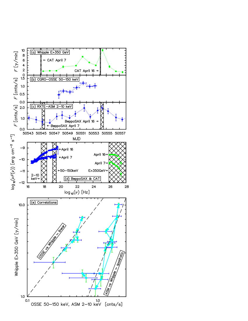
Figure 1: The activity of Mrk 501 observed in 1997 April. The upper panels show the $\gamma$–ray and the X–ray light curves obtained by the Whipple (a), CGRO–OSSE (b) and RXTE–ASM (c) experiments (Catanese et al. catanese97 (1997)). The shaded areas in these figures indicate the observing periods of the $Beppo$SAX and CAT instruments. In panel (d) we show the spectra obtained by the above mentioned instruments (Pian et al. pian98 (1998), Djannati–Atai et al. djannati99 (1999)). In this panel we show also the energy bands used to obtain the light curves. The lower panel (e) shows the two correlations made between the X–ray and the TeV gamma–ray fluxes. For clarity, we multiply the OSSE data in this panel by the factor 0.5. The dashed lines in this panel show a template for the linear and the quadratic correlation.

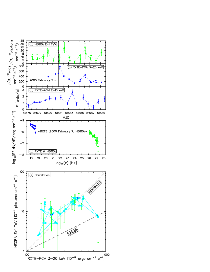
Figure 2: The activity of Mrk 421 observed on 2000 February. The upper panels show the $\gamma$–ray and the X–ray light curves obtained by the HEGRA (a), RXTE–PCA (b) and RXTE–ASM (c) experiments (Krawczynski et al. krawczynski01 (2001)). The shaded areas in these panels indicate the observing periods for the spectra obtained by the RXTE and HEGRA instruments presented in panel (d). The lower panel (e) shows the correlation between the X–ray and the TeV $\gamma$–ray fluxes. The dashed lines in this panel show a template for the linear and the quadratic correlation.                                                                                                                                                                                                                                                       

In Figure 1 we show the activity of Mrk 501 observed in 1997 April. We show in this figure the light curves obtained by the Whipple (E$>$350 GeV), CGRO–OSSE (50–150 keV), and RXTE–ASM (3–20 keV) experiments (Figs 1–a,b,c respectively, Catanese et al. catanese97 (1997)). We show also the evolution of the spectral energy distribution (Fig. 1–d) observed by the $Beppo$SAX (0.1–200 keV) and CAT (E$>$250 GeV) instruments during this activity (Pian et al. pian98 (1998), Djannati–Atai et al. djannati99 (1999)). For this data we calculate two correlations. The first correlation is calculated between the fluxes obtained by the OSSE and the Whipple experiments. This correlation gives an almost linear result (Fig. 1–e). The precise computation gives in this case $F_{\rm{Whipple}}\propto F_{\rm{OSSE}}^{1.71\pm 0.50}$ with a reduced $\chi^{2}=0.67$. The second correlation is calculated between the data from the ASM experiment and the fluxes obtained by the Whipple telescope. This correlation gives a quadratic or even more than quadratic result. The precise computation gives $F_{\rm{Whipple}}\propto F_{\rm{ASM}}^{2.69\pm 0.56}$ and the reduced $\chi^{2}=0.65$. Note that to compare two light curves, where the observational points are randomly distributed in time, it is necessary to select points gathered almost exactly at the same time. This may practically mean that we are able to correlate only a few points in a light curves where we have even dozens of points. In the alternate approach we may try to interpolate one of the light curves. However, this method requires similar sampling of the light curves. Moreover, the sampling should be comparable or less than the characteristic variability time scale of a source. In the case of the OSSE-Whipple correlation we have interpolated the Whipple light curve. The interpolation method in this particular case has a minimal influence on the final result because the OSSE and Whipple observational points were gathered almost at the same time. There is only one point in the OSSE light curve (50549-50550 MJD) which has no counterpart in the TeV observations and we have excluded this point from our analysis. In the ASM-Whipple correlation we have interpolated the ASM light curve. The time shifts between the observational points in these light curves are relatively large in comparison to the previous correlation. However, each point in the ASM light curve has been calculated as an average of many basic measurements made during a period of about one day. Therefore, the interpolation in this case also provides meaningful results. Moreover, our results are in agreement with the previous correlation made by Djannati–Atai et al. (djannati99 (1999)). They obtained a more than linear but less than quadratic correlation between the $Beppo$SAX and the CAT telescope fluxes. Note that the energy range of the $Beppo$SAX observations (0.1–200 keV) covers the spectral bands used by the ASM and the OSSE experiments (Fig. 1–d). Therefore, the correlation mentioned above gives an average of the two correlations presented in this work. The source was observed at that time also by other instruments. Krawczynski et al. (krawczynski00 (2000)) correlated the evolution of the X–ray emission at 3 keV with the evolution of the $\gamma$–ray radiation at 2 TeV. The correlation they obtained seems to be more than quadratic (see Figure 6–a in their paper). This is very similar to the correlation presented here between the ASM (2–10 keV) and the Whipple observations. The second correlation performed by the team mentioned above concerns the evolution of the X–ray emission at 25 keV and the evolution of the $\gamma$–rays at 2 TeV. This correlation gives an almost quadratic result (see Figure 6–b in their article).

The correlations discussed above show that there was significant difference between the evolution of the synchrotron emission before the $\nu F_{s}(\nu)$ peak and the evolution around the peak. It means that the correlation may depend on the position of the spectral bands (below, around or above the $\nu F_{s/c}(\nu)$ peak) used for the calculations. The comparison between our correlations and the correlation done by Djannati–Atai et al. (djannati99 (1999)) indicates that the slope of the correlation may also depend on the width of the spectral band.

In Figure 2 we present the activity of Mrk 421 observed in 2000 February. We show the light curves gathered by the HEGRA (E$>$1TeV), RXTE–PCA (3–20 keV) and the RXTE–ASM (2–10 keV) experiments (Figs 1–a,b,c respectively, Krawczynski et al. krawczynski01 (2001)). We show also the spectral energy distributions observed at that time (Fig. 1–d). We calculate for this source the correlation between the PCA and the HEGRA fluxes. To obtain the correlation we have interpolated the HEGRA light curve. However, the interpolation as in the case of the OSSE-Whipple correlation for Mrk 501, has minimal influence on the result because the observations in both light curves were made almost simultaneously. In this case we have obtain unclear results; the detailed fitting gives $F_{\rm{HEGRA}}\propto F_{\rm{PCA}}^{0.47\pm 0.15}$ with a poor reduced $\chi^{2}$ of 1.7. Note that also the correlation between the ASM and the HEGRA data, which we do not present here, does not provide an informative result. This example shows that the relatively long timescale observations with one data point per day may not be sufficient to obtain meaningful information on the TeV/X–ray correlation.

However, Fossati et al. (fossati04 (2004)) have recently reported very precise observations of this source made in 2001 March. The object was observed during a period of one week by the RXTE–PCA, Whipple and the HEGRA instruments. The rate of the measurements was relatively high and several flaring events were well observed. The most significant seems to be a flare observed on March 19 by the PCA and Whipple instruments. The TeV/X–ray correlation for this flare is almost quadratic ($F_{\rm TeV}\propto F_{\rm X}^{2.3\pm 0.3}$) for the rising and decaying phase. However, the correlation for data obtained by the Whipple and RXTE–PCA experiments during this campaign gives $F_{\rm TeV}\propto F_{\rm X}^{1.3\pm 0.1}$. This indicates that the longterm correlation may give results significantly different from the correlation performed for one single flaring event. The reason for the difference may be related to the fact that for a long term light curve (e.g. a few days or even longer) we may correlate at least a few flaring events. If for example the activity is generated in the framework of the internal shock mechanism (e.g. Rees rees78 (1978), Guetta et al. guetta04 (2004)) then the flares may overlap each other in time. If we observe a decay phase of a flare and during this decay a new flare will start to rise then the observed correlation would be completely different even if the base correlation for each flare was the same.

Recently Tanihata et al. (tanihata04 (2004)) published a spectral analysis of the observations of Mrk 421 obtained during a 7 day campaign in 1998. They found a correlation between the TeV flux and the synchrotron peak flux $F_{\rm TeV}\propto F_{\rm s,peak}^{1.7\pm 0.3}$.

In the following we will take particular care in looking for robust solutions yielding linear or quadratic correlations between X-ray and TeV bands. Although so far there are only few cases for which these correlations (especially the quadratic one) have been clearly established, our attention is motivated by the fact that, as we will discuss below, the observations of such a correlations could impose strong constraints on the scenario usually considered for the variability observed in these sources. In particular the observation of a quadratic relation during the decaying phase is particularly intriguing. In fact, if the quadratic increase of the synchrotron and IC emission could be easily reproduced, increasing the electron density within the source, the decrease is more problematic. Escape of electrons from the sources appears unrealistic in the small timescale shown by variability. On the other hand radiative cooling can affect only the high-energy particles. Indeed, the simple quadratic relation predicted for the IC emission is strictly valid for IC in the Thomson regime. However, the TeV emission of the HBL objects is probably generated in the Klein-Nishina regime. In Appendix A we estimate the physical parameters of a source that could generate TeV emission in the Thomson limit. The estimation gives unacceptably large values of the Doppler factor ($\delta\gtrsim 1000$, Begelman et al. begelman94 (1994)). Therefore, in all models presented in this work we assume that the TeV radiation comes from the IC scattering in the Klein-Nishina regime. The decline of the cross-section in the Klein-Nishina regime (valid for sources with a plausible value of the physical quantities) has the effect of decoupling the (high-energy) electrons producing the high-energy photons and those (at low-energy) producing the optical–IR synchrotron seed photons (e.g. Tavecchio, Maraschi & Ghisellini 1998). In these conditions, since the radiative cooling only affects the high-energy particles, a linear relation between X-rays and TeV should be expected, since the seed photons can be considered almost constant during the decay. A plausible alternative, discussed in detail below, is to admit adiabatic cooling, affecting all the electrons, irrespective of their energy.

3 Spherical homogeneous source

A homogeneous synchrotron-SSC model is frequently proposed as a possible explanation for the X–ray and the $\gamma$–ray emission of HBL objects. Such model provide a very good and simple explanation for the Spectral Energy Distributions (SED) observed in X–rays and the TeV gamma rays (e.g. Dermer $\&$ Schlickeiser dermer93 (1993), Bednarek $\&$ Protheroe bednarek97 (1997), Mastichiadis & Kirk mastichiadis97 (1997), Pian et al. pian98 (1998), Katarzyński et al. katarzynski01 (2001)). Therefore, we decided to check if such a model is also able to explain quite specific properties of the observed variability. In the approach presented in this section we do not consider Light Crossing Time Effects (hereafter LCTE) in the synchrotron radiation field inside the source nor for the total observed emission. This means that the results presented in this section are strictly valid only if the physical processes, which modify the source brightness, are slower than the source light crossing time. This condition may not always be correct in the case of blazars. However, it allows us to investigate in detail the most important physical processes which may modify the emission level of the source. Detailed understanding of these processes is very important for any more complex modeling.

3.1 Description of the model

We assume for this modeling a spherical homogeneous source, which may undergo expansion or compression. As a first step, to simplify the model and to provide analytical formulae which describe the evolution of such a source, we decided to consider only four physical processes which may occur during the evolution. We calculate increase or decrease of the source volume, increase or decay of the magnetic field intensity, variations of the particle density and adiabatic heating or cooling of the particles. In the model we separate as much as possible the mathematical description for each process. This allows us to investigate separately the influence of each process on the source emission. In this first approach we do not consider the radiative cooling of the particles. The impact of this process will be discussed in the next part of this work (Subsection 3.7).

The time evolution of the source radius ($R$) and the magnetic field intensity ($B$) are assumed to be a power law functions

$$R(t)=R_{0}\left(t_{0}/t\right)^{-r_{e}},\leavevmode\nobreak\ \leavevmode\nobreak\ \leavevmode\nobreak\ \leavevmode\nobreak\ \leavevmode\nobreak\ B(t)=B_{0}\left(t_{0}/t\right)^{m},$$ (1)

where $t_{0}$, $R_{0}$ and $B_{0}$ are initial time, magnetic field intensity and radius respectively. The indices $r_{e}$ and $m$ are a free parameters in our modeling.

The initial ($t=t_{0}$) distribution of the electron energy inside the source is defined by a broken power law

$$N_{0}(\gamma)=\left\{\begin{array}[]{ll}k_{1}\gamma^{-n_{1}},&\mbox{$\gamma_{\rm min}\leq\gamma\leq\gamma^{0}_{\rm brk}$}\\ k_{2}\gamma^{-n_{2}},&\mbox{$\gamma^{0}_{\rm brk}\leavevmode\nobreak\ <\gamma\leq\gamma_{\rm max}$}\\ \end{array}\right.,$$ (2)

where $k_{2}=k_{1}(\gamma^{0}_{\rm brk})^{n_{2}-n_{1}}$, $\gamma$ is the Lorentz factor which is equivalent to the electron energy, $\gamma^{0}_{\rm brk}$ describes initial position of the break, $n_{1}$ and $n_{2}$ are spectral indices before and above the break respectively. In the model we assume that the dominant part of the X-ray and TeV emission is produced by the electrons with the Lorentz factors around $\gamma_{\rm brk}$. Therefore, the values of $\gamma_{\rm min}$ and $\gamma_{\rm max}$ parameters are not important for the results of the modeling. For all calculations presented in this section we use $\gamma_{\rm min}=1$ and $\gamma_{\rm max}=10^{8}$.

The evolution of the electron energy spectrum is defined by a minimum

$$N(\gamma,t)=\min\left\{N_{1}(\gamma,t),N_{2}(\gamma,t)\right\}$$ (3)

of two power law functions

$$\begin{array}[]{ll}\vspace*{0.2cm}N_{1}(\gamma,t)=K_{1}(t)\gamma^{-n_{1}};&\leavevmode\nobreak\ \leavevmode\nobreak\ \leavevmode\nobreak\ \leavevmode\nobreak\ \leavevmode\nobreak\ K_{1}(t)=k_{1}\left(\frac{t_{0}}{t}\right)^{3r_{d}}\left(\frac{t_{0}}{t}\right)^{r_{a}(n_{1}-1)},\\ N_{2}(\gamma,t)=K_{2}(t)\gamma^{-n_{2}};&\leavevmode\nobreak\ \leavevmode\nobreak\ \leavevmode\nobreak\ \leavevmode\nobreak\ \leavevmode\nobreak\ K_{2}(t)=k_{2}\left(\frac{t_{0}}{t}\right)^{3r_{d}}\left(\frac{t_{0}}{t}\right)^{r_{a}(n_{2}-1)},\\ \end{array}$$ (4)

where $K_{1}$ and $K_{2}$ describe the evolution of the particle density before and after the break ($\gamma_{brk}$). The exponent $3r_{d}$ describes the decrease or increase of the particle density. The adiabatic heating or cooling of the particles is described by the indices $r_{a}(n_{1|2}-1)$. Note that if we assume for example adiabatic expansion or compression of the source with a constant number of the particles, then the parameters $r_{e}$, $r_{d}$ and $r_{a}$ should be equal (e.g. Kardashev kardashev62 (1962), Longair longair92 (1992)). This is in fact the most realistic case. However, to investigate separately the influence of the above mentioned processes, we decided to produce such a detailed parameterization.

Assuming that the electron spectrum is defined by the minimum of two evolving power law functions we can easily find the evolution of the break $\gamma_{\rm brk}(t)=\gamma^{0}_{\rm brk}\left(t_{0}/t\right)^{r_{a}}.$

3.1.1 Synchrotron emission

The synchrotron emission coefficient which describes the radiation of the electrons is given by the well-known formula $j_{s}\propto KB^{(\alpha+1)}$ (e.g. Rybicki $\&$ Lightman rybicki79 (1979)) where $\alpha=(n-1)/2$. In our particular case we have to define the evolution of two emission coefficients

$$j^{1|2}_{s}(t)\propto K_{1|2}(t)B(t)^{(\alpha_{1|2}+1)}\propto k_{1|2}B_{1|2}\left(\frac{t_{0}}{t}\right)^{3r_{d}+r_{a}(n_{1|2}-1)+m(\alpha_{1|2}+1)},$$ (5)

where $j^{1}_{s}$ describes emission of the low energy electrons ($\gamma<\gamma_{brk}$), $j^{2}_{s}$ describes the radiation of the high energy electrons ($\gamma>\gamma_{brk}$) and $B_{1|2}=B_{0}^{\alpha_{1|2}+1}$.

In our modeling we neglect the electron self–absorption process which is important only for the emission at the radio frequencies which we do not analyze in this work. Therefore, we can approximate the evolution of the intensity of the synchrotron radiation from the spherical source by

$$I^{1|2}_{s}(t)\propto R(t)j^{1|2}_{s}(t)\propto R_{0}k_{1|2}B_{1|2}\left(\frac{t_{0}}{t}\right)^{-r_{e}+3r_{d}+r_{a}(n_{1|2}-1)+m(\alpha_{1|2}+1)}.$$ (6)

Finally we can write the evolution of the synchrotron flux multiplying the intensity by the source surface

$$\vspace*{0.1cm}F^{1}_{s}(t) \propto R^{2}(t)I^{1}_{s}(t)\leavevmode\nobreak\ \propto\leavevmode\nobreak\ R_{0}^{3}k_{1}B_{1}\left(\frac{t_{0}}{t}\right)^{-s_{1}},$$ (7)

$$s_{1} = 3r_{e}-3r_{d}-r_{a}(n_{1}-1)-m(\alpha_{1}+1),$$ (8)

$$\vspace*{0.1cm}F^{2}_{s}(t) \propto R^{2}(t)I^{2}_{s}(t)\leavevmode\nobreak\ \propto\leavevmode\nobreak\ R_{0}^{3}k_{2}B_{2}\left(\frac{t_{0}}{t}\right)^{-s_{2}},$$ (9)

$$s_{2} = 3r_{e}-3r_{d}-r_{a}(n_{2}-1)-m(\alpha_{2}+1),$$ (10)

where the indices $s_{1}$ and $s_{2}$ describe the evolution of the synchrotron emission generated by the low and the high energy electrons respectively. Note that there is a difference between the evolution of the $F^{1}_{s}$ flux and the evolution of the $F^{2}_{s}$ radiation due to the adiabatic processes ($r_{a}(n_{1|2}-1)$) and the evolution of the magnetic field intensity ($m(\alpha_{1|2}+1)$).

3.1.2 Self Compton emission

Tavecchio et al. (tavecchio98 (1998)) presented detailed studies of the SSC emission generated by the electrons with an energy spectrum approximated by a broken power law. The IC spectrum in such an approach can be divided into four basic components ($F^{1...4}_{c}$). However, only two of them are dominant in the IC emission generated by HBL objects. The first dominant component ($F^{1}_{c}$) is generated by the low energy electrons ($K_{1},N_{1}$) and the first part of the synchrotron spectrum ($I^{1}_{s},F^{1}_{s}$). The second important component ($F^{2}_{c}$) is produced by the high energy electrons ($K_{2},N_{2}$) and the first part of the synchrotron emission ($I^{1}_{s},F^{1}_{s}$). With these results in mind, we can derive the formulae describing the evolution of emission coefficients for the dominant components

$$j^{1}_{c}(t)\propto K_{1}(t)I^{1}_{s}(t)\propto R_{0}k_{1}^{2}B_{1}\left(\frac{t_{0}}{t}\right)^{-r_{e}+6r_{d}+2r_{a}(n_{1}-1)+m(\alpha_{1}+1)}.$$ (11)

$$j^{2}_{c}(t) \propto K_{2}(t)I^{1}_{s}(t)$$ (12)

$$\propto R_{0}k_{1}k_{2}B_{1}\left(\frac{t_{0}}{t}\right)^{-r_{e}+6r_{d}+r_{a}(n_{2}-1)+r_{a}(n_{1}-1)+m(\alpha_{1}+1)}.$$

By analogy to the synchrotron emission we can write the evolution of the intensity of the IC emission for both the discussed cases $I^{1|2}_{c}(t)\propto R(t)j^{1|2}_{c}(t).$ The evolution of the IC flux is given then by

$$\vspace*{0.1cm}F^{1}_{c}(t) \propto R^{2}(t)I^{1}_{c}(t)\leavevmode\nobreak\ \leavevmode\nobreak\ \propto\leavevmode\nobreak\ \leavevmode\nobreak\ R_{0}^{4}k^{2}_{1}B_{1}\left(\frac{t_{0}}{t}\right)^{-c_{1}},$$ (13)

$$c_{1} = 4r_{e}-6r_{d}-2r_{a}(n_{1}-1)-m(\alpha_{1}+1),$$ (14)

$$\vspace*{0.1cm}F^{2}_{c}(t) \propto R^{2}(t)I^{2}_{s}(t)\leavevmode\nobreak\ \leavevmode\nobreak\ \propto\leavevmode\nobreak\ \leavevmode\nobreak\ R_{0}^{4}k_{1}k_{2}B_{1}\left(\frac{t_{0}}{t}\right)^{-c_{2}},$$ (15)

$$c_{2} = 4r_{e}-6r_{d}-r_{a}(n_{1}-1)-r_{a}(n_{2}-1)-m(\alpha_{1}+1),$$ (16)

where $c_{1}$ describes the evolution of the IC radiation in the Thomson limit and $c_{2}$ describes the evolution of the IC emission in the Klein–Nishina regime.

3.1.3 Components of the synchrotron self Compton spectrum: an example

To show that the approximations used in the derivation of the equations describing the SSC emission are correct, in Figure 3 we report an example of the evolution of the synchrotron and the IC emission generated by the expanding spherical homogeneous source, calculated using our numerical code. The results presented in this subsection are correct for a wide range of values of the physical parameters usually assumed in order to explain the X-ray and TeV emission of the HBL objects. However, the results are correct only for case where the dominant part of the synchrotron and the IC emission (the peaks) is generated by electrons with the Lorentz factors close to $\gamma_{\rm brk}$ which practically means $n_{2}>3$. The spectra presented in Figure 3 are divided into different components. This test shows that indeed only two components are important for the high energy IC emission for a large amplitude of the variation. Note that the components are calculated numerically, therefore the spectra shown are slightly different from the curves obtained from the analytical approximations by Tavecchio et al. (tavecchio98 (1998)). For the numerical calculations we use the SSC emission mechanism described by Katarzyński et al. (katarzynski01 (2001)). In the test we use following parameters $\delta=50$, $R_{0}=2\times 10^{16}$ [cm], $B_{0}=0.004$ [G], $k_{1}=10^{3}$ [cm${}^{-3}]$, $\gamma_{\rm min}=1$, $\gamma_{\rm brk}=1.2\times 10^{6}$, $\gamma_{\rm max}=10^{8}$, $r_{e}=r_{d}=r_{a}=m=1$. Note that in an ideal case where the source is perfectly spherical and homogeneous and the magnetic field inside the source is well organized the parameter $m$ which describes the evolution of the magnetic field should be equal to $2r_{e}$ (e.g. $m=2$ for a linear expansion of the source) in order to keep the magnetic flux constant.

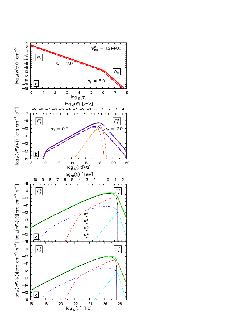
Figure 3: The evolution of the synchrotron and the IC emission of an expanding spherical homogeneous source. Panel (a) shows the evolution of the electron energy spectrum. The spectrum gives the synchrotron radiation shown in panel (b). The evolution of the IC spectrum is shown in panels (c) and (d). To simplify the figures we show only the initial and the final spectra. Note that the initial spectra in all figures are shown by bold–solid lines while the spectra generated at the end of the simulation are shown by bold–dashed lines. The basic components of the emission are shown by various thin lines. A detailed description of the components and the parameters used for the test are given in subsection 3.1.

However, practically the occurrence of such ideal sources is very unlikely. Usually we would expect a more complex geometry, inhomogeneity and a turbulent magnetic field inside the source which may give a more complex evolution of the magnetic field. For example a slower than expected decrease of the magnetic field during the expansion may be caused by the turbulent dynamo effect (e.g. Atoyan & Aharonian atoyan99 (1999) for discussion of this problem). Therefore, we assume the parameter $m$ to be a free parameter in our modeling. For the linear expansion we assume that the value of this parameter may vary from 1 to 2. The value of this parameter has no influence on the results presented in this subsection. However, in other tests presented in the next part of this work, we had to use $m=1$ in order to explain the quadratic correlation observed in the decaying phase of the flare. Therefore, to be consistent and to provide the possibility of comparison of the results, in all numerical calculations presented in this paper we have selected $m=1$. Moreover, in this test and in all other simulations presented in this work we assume that the $t_{0}$ parameter is equal to $10\leavevmode\nobreak\ R_{0}/c$. This gives the radius expansion velocity equal to $0.1c$ for $r_{e}=1$. To change the source emission level at least a few times we simulate the evolution for a period of time equal to $3\leavevmode\nobreak\ R_{0}/c$. This set of parameters is quite specific because we use a relatively small value of the initial magnetic field and a relatively large value of the Doppler factor (see estimations made by Tavecchio et al. tavecchio98 (1998) or Katarzyński et al. katarzynski01 (2001)). We assume a small value of the magnetic field in order to neglect radiative cooling, which cannot be described easily by the analytical formulae. On the other hand, to reach the observed level of emission, we have to assume a large value of the Doppler factor. The Doppler factor value $\geq 50$ has been used by some authors (e.g. Krawczynski et al. krawczynski02 (2002), Konopelko et. al. konopelko03 (2003)) to explain the emission of TeV blazars. We will prove in the next part of this work (Subsection 3.7) that the radiative cooling is indeed negligible for this set of parameters. In this test the radiative cooling is negligible for electrons with the energy described by the Lorentz factor around $\gamma_{\rm brk}$ which are producing the dominant part of the emission observed as the synchrotron and IC peaks. On the other hand the radiative cooling is still important for electrons with a Lorentz factor around $\gamma_{\rm max}$. However, the radiation generated by these particles is almost completely negligible due to the steepness of their spectrum.

Moreover, for this test and for other calculations presented in this work we use the Hubble constant equal to 65 [km s^-1 Mpc^-1] and the redshift equal to 0.03. In the above calculations and in all other calculations of the IC scattering presented in this work, we neglect the possible absorption of the $\gamma$–ray emission due to pair production inside the source. This process can be neglected if the Doppler factor of the source is of the order of ten or more (e.g. Bednarek & Protheroe bednarek97 (1997)). Moreover, to calculate the observed TeV flux, we should also consider the absorption of this radiation by interaction with the Infrared Intergalactic Background. However, in this particular case, we are mainly interested in investigating the evolution of the TeV radiation with respect to the evolution of the synchrotron X–ray emission. Therefore, absorption of the TeV emission by the IR background, which is constant in time, does not modify the TeV/X–ray flux correlation.

3.2 Basic cases

Correlating the X–ray and TeV emission of the HBL objects we can distinguish two general cases. In the first case we compare the X–ray emission before the synchrotron peak ($F^{1}_{s}$) with the $\gamma$–ray radiation above the IC peak ($F^{2}_{c}$, e.g. Mrk 501, Figure 1). In the second case we correlate the X–ray emission above the synchrotron peak ($F^{2}_{s}$) with the $\gamma$–ray radiation above the IC peak ($F^{2}_{c}$, e.g. Mrk 421, Figure 2). To simplify the discussion presented in this work we hereafter call these correlations $c_{2}/s_{1}$ and $c_{2}/s_{2}$ respectively. We also present in this section the estimates of other possible correlations ($F^{1}_{s}$ vs $F^{1}_{c}$ and $F^{2}_{s}$ vs $F^{1}_{c}$). However, we will not discuss them in detail. The more complex cases of the TeV/X–ray correlation, where the considered bands correspond to the emission around the peaks, discussed in subsection 3.5.

For the tests presented in this section we use the same values of the physical parameters as in the calculations presented in the previous subsection. To simulate different evolution scenarios we change only four model parameters $r_{e},r_{d},r_{a},m$ setting 0 or 1 as the value for these parameters. This means that in principle we can study only expansion of the source. However, as long as we neglect the radiative cooling, the results of such tests are opposite to the results which we could obtain from the compression of the source. Having four parameters and two possible values for these parameters (0 or 1) we have in principle sixteen different combinations ($2^{4}$). However, one combination is not interesting ($r_{e}=r_{d}=r_{a}=m=0$) and four other combinations are not realistic (all cases where we should calculate the adiabatic cooling without a decrease of the particle density). In Table 1 we show eleven other possible combinations plus one test where we use $m=2$.

We discuss here in detail only a few tests which we consider to be the most realistic:

• In our first case (Table 1–$a$) we assume the expansion of the source volume ($r_{e}=1$) with constant particle density and magnetic field intensity ($r_{d}=m=0$). This scenario could correspond to a constant injection of particles (e.g. from a shock region) which extends the dimension of the source instead of increasing the particle density. The synchrotron radiation in this case is proportional to the source volume. Therefore, the synchrotron emission produced by the low and the high energy electrons increases with time as $R^{3}\propto t^{3r_{e}}$ ($s_{1|2}=3$. Eqs 7,  9). The IC radiation in this test is also proportional to the source volume. However, the IC emission is also proportional to the intensity of the synchrotron emission (Eq. 6) which grows linearly with the radius of the source ($I^{1|2}_{s}\propto Rj^{1|2}_{s}\propto t^{r_{e}}$). Therefore, the IC radiation increases in time as $t^{3r_{e}+r_{e}}$ ($c_{1|2}=4$). Finally we obtain $c_{1|2}/s_{1|2}=4/3$ for all possible correlations.

• The second case ($b$) is opposite to the scenario just described. We increase the particle density ($r_{d}=1$) keeping the volume and the magnetic field intensity constant ($r_{e}=m=0$). A linear increase of the density provides a linear increase of the synchrotron radiation. The IC emission is proportional to the density of the particles and to the intensity of the synchrotron radiation which is also proportional to the density. Therefore, the IC emission is proportional to the square of the particle density. This is well-known relation. In this particular case we obtain a quadratic correlation in all possible cases ($c_{1|2}/s_{1|2}=2/1$).

  Table 1: Estimated correlation between evolution of the synchrotron emission and the evolution of the IC emission for different evolutionary scenarios. Columns 2–5 show the parameters used for the tests. Columns 6–9 show the estimated values of the correlation in four possible cases ($c_{1|2}/s_{1|2}$).

  case	$r_{e}$	$r_{d}$	$r_{a}$	$m$	$c_{1}/s_{1}$	$c_{1}/s_{2}$	$c_{2}/s_{1}$	$c_{2}/s_{2}$
  $a$	1	0	0	0	1.333	1.333	1.333	1.333
  $b$	0	1	0	0	2	2	2	2
  $c$	1	1	0	0	inf	inf	inf	inf
  $d$	1	1	1	0	4	1	7	1.75
  $e$	1	1	1	1	2.2	0.786	3.4	1.214
  $f$	0	0	0	1	1	0.5	1	0.5
  $g$	0	1	1	0	2	1.143	2.75	1.571
  $h$	0	1	1	1	1.727	0.950	2.273	1.250
  $i$	1	1	0	1	2.332	1.167	2.333	1.167
  $j$	1	0	0	1	1.667	inf	1.667	inf
  $k$	0	1	0	1	1.667	1.250	1.667	1.250
  $l$	1	1	1	2	1.75	0.7	2.5	1

• In the next case ($d$) we assume an increase of the volume, decrease of the particle density and with adiabatic cooling ($r_{e}=r_{d}=r_{a}=1$) with a constant value of the magnetic field intensity ($m=0$) during the evolution. Even if it is rather unlikely that the magnetic field can remain constant, we describe this case to provide a sort of introduction to our last, more complex test. The synchrotron emission decreases in this test due to the adiabatic losses because the decrease of the density is fully compensated for the increase in the volume if $r_{e}=r_{d}$. This decrease depends on the slope ($n_{1|2}$) of the particle spectrum (Eq. 4). The synchrotron emission produced by the low energy electrons decreases more slowly ($t^{-r_{a}(n_{1}-1)}$, $s_{1}=-1$) than the emission generated by the high energy electrons ($t^{-r_{a}(n_{2}-1)}$, $s_{2}=-4$). The IC emission also decreases in this test. In the Thomson limit, the IC flux is proportional to the increase in the volume ($t^{3r_{e}=3}$) and the radius ($t^{r_{e}=1}$, which comes from the intensity of the synchrotron emission $I^{1}_{s}\propto Rj^{1}_{s}\propto t^{r_{e}}$) and also to the square of the density of the low energy electrons including the adiabatic losses ($K_{1}^{2}\propto t^{-6r_{d}-2r_{a}(n_{1}-1)=-8}$). This finally gives $c_{1}=-4$. In the Klein–Nishina regime the IC radiation is proportional to the evolution of the volume and radius as in the previous case ($t^{3r_{e}+r_{e}=4}$). However, this time the scattering is proportional to the density of the low energy electrons including the adiabatic losses ($K_{1}\propto t^{-3r_{d}-r_{a}(n_{1}-1)=-4}$, which comes from the intensity of synchrotron radiation $I^{1}_{s}$) and is proportional to the density of the high energy electrons including the adiabatic losses ($K_{2}\propto t^{-3r_{d}-r_{a}(n_{2}-1)=-7}$). As a result, the IC flux in the Klein–Nishina regime decreases as $t^{-7}$ ($c_{2}=-7$). The influence of the adiabatic losses provides in this test four different correlations $c_{1}/s_{1}=4$, $c_{1}/s_{2}=1$, $c_{2}/s_{1}=7$, $c_{2}/s_{2}=1.75$.

• In our last test ($e$) we assume an increase of the source radius, the decrease of the particle density with adiabatic cooling and also decay of the magnetic field ($r_{e}=r_{d}=r_{a}=m=1$). The decrease of the magnetic field causes a much faster decrease of the synchrotron emission ($t^{-r_{a}(n_{1|2}-1)-m(\alpha_{1|2}+1)}$, $s_{1}=-2.5$, $s_{2}=-7$) in comparison to the previous case. Moreover, this decrease increases the difference between the synchrotron emission produced by low and high energy electrons. The IC emission decreases faster as well. However, the factor ($t^{-m(\alpha_{1}+1)=-1.5}$) which marks the difference to the evolution discussed in our previous test is the same for the emission in the Thomson and in the Klein–Nishina regime. This is a consequence of the fact that the $\gamma$–rays in the Thomson and Klein–Nishina regime are produced by the scattering of the synchrotron radiation field produced by the low energy electrons ($I^{1}_{s}$). Therefore, the decay of the magnetic field does not modify the difference between the two scattering regimes. In conclusion, we have to add the factor –1.5 (with respect to the previous case) to the indices describing the evolution of the IC emission, to obtain $c_{1}=-5.5$ and $c_{2}=-8.5$. Also in this case we obtain four different values for the correlations $c_{1}/s_{1}=2.2$, $c_{1}/s_{2}=0.786$, $c_{2}/s_{1}=3.4$, $c_{2}/s_{2}=1.214$.

For all estimations presented in this subsection we have assumed constant values for the parameters $n_{1}$ and $n_{2}$. However, we have checked also that for the most realistic scenarios ($e$ & $l$) and for all combinations of the $n_{1}$ value in the range from 1.5 to 2.5 and the $n_{2}$ value in the range from 3 to 8, the correlation $c_{2}/s_{1}$ is always more than quadratic while the correlation $c_{2}/s_{2}$ is always less than quadratic. We provide also a simple mathematical formulae for these realistic evolutions

$$\begin{array}[]{lcccl}\vspace{0.4cm}c_{2}/s_{1}=&{\frac{\displaystyle 1+3n_{1}+2n_{2}}{\displaystyle 3n_{1}-1}}&\mathrm{or}&\frac{\displaystyle 1+2n_{1}+n_{2}}{\displaystyle 2n_{1}}&\textrm{TeV vs soft X--rays}\\ c_{2}/s_{2}=&\underbrace{\frac{1+3n_{1}+2n_{2}}{3n_{2}-1}}_{m=1}&\mathrm{or}&\underbrace{\frac{1+2n_{1}+n_{2}}{2n_{2}}}_{m=2}&\textrm{TeV vs hard X--rays}\\ \end{array}$$

3.3 Problem with “the quadratic decay”

This concerns the quadratic results of the $c_{2}/s_{2}$ correlations during the decay phase of the flare. Within the scenarios proposed in the previous subsection there is only one solution that may explain exactly the quadratic correlation (see column marked $c_{2}/s_{2}$ in Table 1). However, this well-known test assumes only variations of the particle density. Therefore, this scenario can be easily used to explain the rising phase of the flare, where the activity is generated for instance by the injection of the particles into a constant volume of the source. We cannot easily explain the decrease of the density during the decay of the flare. In principle such a decrease could be related to the escape of the particles into a region where the magnetic field intensity is significantly less than inside the source. However, this process does not guarantee that the efficiency of the total IC emission will decrease two times faster than the efficiency of the synchrotron radiation. The IC scattering may also occur efficiently in the region where the magnetic field is significantly less, especially close to the source surface (distance $\lesssim 1.5R$), where the radiation field energy density is on average only two times less than on the source surface (Gould gould79 (1979)). The decrease of the density could be also related to the expansion of the source. However, assuming the expansion we have to consider also the influence of some additional physical process. We have to consider the adiabatic cooling of the particles and probably also the decay of the magnetic field. All these processes can destroy the quadratic correlation which is related to the variation of the density. Each additional physical process which can modify the evolution of the synchrotron and the IC emission ($F_{s|c}\propto t^{s|c}$) in the same way ($t^{s|c+x}$) can destroy this correlation. This is a consequence of the simple fact that if $c/s=2$ then $(c+x)/(s+x)\neq 2$. If the influence of the additional process is different for the evolution of the synchrotron emission ($t^{s+x}$) and for the evolution of the IC radiation ($t^{c+y}$) then we have situations where $(c+y)/(s+x)$ should give 2 if we want to keep the quadratic correlation. Therefore, assuming $s=-1$ and $c=-2$, which is a simple consequence of the decrease of the density, we obtain a simple relation $y=2x$ which should be fulfilled by the additional physical process to keep the quadratic correlation. For example the adiabatic cooling gives $x=-r_{a}(n_{2}-1)$ for the evolution of $F^{2}_{s}$ and $y=-r_{a}(n_{1}-1)-r_{a}(n_{2}-1)$ for the evolution of $F^{2}_{c}$. Therefore, the relation $y=2x$ can be fulfilled only if $n_{1}=n_{2}$ which does not provide the correct solution. The efficiency of the synchrotron emission depends among other things on the slope of the particle spectrum and the intensity of the magnetic field. Therefore, the decay of the magnetic field gives $x=-m(\alpha_{2}+1)$ for the evolution of $F^{2}_{s}$ and $y=-m(\alpha_{1}+1)$ for the evolution of $F^{2}_{c}$. Therefore, the relation can be fulfilled if $\alpha_{1}=2\alpha_{2}$ which also does not give the correct solution. Moreover, we have to stress that the decay of the magnetic field always results in a much faster decay of the second part of the synchrotron radiation than the decay of the IC emission in the Klein–Nishina regime and the Thomson limit as well. In principle this unwanted effect can be compensated by the adiabatic cooling which increases the decrease speed of the $F^{2}_{c}$ flux in comparison to the decrease of the $F^{2}_{s}$ flux. However, detailed computations show that the adiabatic cooling cannot fully compensate the influence of the decay of the magnetic field; compare the correlations for the cases $d$ ($r_{e}=r_{d}=r_{a}=1,m=0$), $e$ ($r_{e}=r_{d}=r_{a}=m=1$ and $l$ ($r_{e}=r_{d}=r_{a}=1,m=2$) in Table 1.

3.4 Change of the Doppler factor

It is possible that in TeV sources the Doppler factor $\delta$ changes during a single flare. Evidence for this come from the requirement of a large $\delta$–value for the inner parts of the jet, generating most of the emission ($\delta\geq 10$, e.g. Dondi & Ghisellini dondi95 (1995), Tavecchio et al. tavecchio98 (1998), Kino et al. kino02 (2002), Ghisellini et al. ghisellini02 (2002), Katarzyński et al. katarzynski03 (2003), or even $\delta\sim 50$, Krawczynski krawczynski02 (2002), Konopelko et al. konopelko03 (2003)), while instead at the VLBI scale ($\sim$sub–pc, including satellite VSOP data) there is no evidence of superluminal motion of the jet’s components (e.g. Piner et al. piner99 (1999), Edwards & Piner edwards02 (2002), Piner & Edwards piner04 (2004), Giroletti et al., giroletti04 (2004)). This suggests a strong deceleration of the source.

To analyze the impact of the change of the Doppler factor for the observed TeV/X–ray correlation we assume the following evolution for $\delta(t)$

$$\delta(t)=\delta_{0}\left(\frac{t_{0}}{t}\right)^{d},$$ (17)

where $d$ is a free parameter. The Doppler boosting effect may change the level of the emission [$F(\nu)\propto\delta^{3}F^{\prime}(\nu^{\prime})$] and the observed frequency ($\nu\propto\delta\nu^{\prime}$). For a power law spectrum ($F^{\prime}\propto\nu^{\prime-\alpha}$) we then have

$$F(\nu,t)=\delta(t)^{3+\alpha}F^{\prime}(\nu,t)\propto\delta_{0}t^{-d(3+\alpha)}F^{\prime}(\nu,t)$$ (18)

Note that the evolution of the flux at given frequency depends not only on the value of the Doppler factor, but also on the spectral index $\alpha$. Therefore, the evolution of the synchrotron emission can be different below and above the peak ($F^{1|2}_{\rm s}\propto\nu^{-\alpha_{1|2}}$). Also the evolution of the IC radiation depends on the spectral index ($F^{1|2}_{\rm c}\propto\nu^{-\alpha_{1|{\rm KN}}}$, where $\alpha_{\rm KN}\sim 2\alpha_{2}-\alpha_{1}$, see Tavecchio et al. tavecchio98 (1998)).

We can describe the IC and synchrotron flux evolution due to the change of the Doppler factor by the $y$ and $x$ coefficients respectively. In this way the correlation which includes the change of $\delta$ becomes $c^{\prime}/s^{\prime}=(c+y)/(s+x)$. The change of $\delta$ will not modify the original ($c/s$) correlation if $y/x=c/s$. Values $y/x>c/s$ makes the new correlation $c^{\prime}/s^{\prime}$ steeper ($c^{\prime}/s^{\prime}>c/s$), and values of $y/x<c/s$ makes the new correlation $c^{\prime}/s^{\prime}$ flatter. This simple estimate shows that the decrease of $\delta$ can help to solve the problem of the quadratic decay, but only slightly, since the change of the slope of the correlation (for actual values of the synchrotron and IC spectral indices) is only mild.

The coefficient $y$ for the evolution of the IC emission in the Klein–Nishina regime is given by $y_{2}=-3d-2d\alpha_{2}+d\alpha_{1}$. The parameter $x$ for the evolution of the synchrotron emission below ($x_{1}$) and above ($x_{2}$) the peak is defined by $x_{1|2}=-3d-d\alpha_{1|2}$. Setting $\alpha_{1}=0.5$, $\alpha_{2}=2$, and $\alpha_{\rm KN}=3.5$, as in the previous modeling, and assuming $d=1$, we obtain $y_{2}/x_{1}=1.857$ and $y_{2}/x_{2}=1.3$. For the most realistic evolution scenarios, cases $e$ and $l$ in the Table 1, we obtain a decrease of the $c_{2}/s_{1}$ correlation slope ($[c_{2}/s_{1}=3.4\to c^{\prime}_{2}/s^{\prime}_{1}=2.5]_{e}$ and $[c_{2}/s_{1}=2.5\to c^{\prime}_{2}/s^{\prime}_{1}=2.2]_{l}$) and a small increase of the $c_{2}/s_{2}$ correlation slope ($[c_{2}/s_{2}=1.214\to c^{\prime}_{2}/s^{\prime}_{2}=1.25]_{e}$ and $[c_{2}/s_{2}=1\to c^{\prime}_{2}/s^{\prime}_{2}=1.1]_{l}$).

This simple estimate shows that the impact of the change of the Doppler factor is much stronger for the $c_{2}/s_{1}$ correlation than for the $c_{2}/s_{2}$ relation. This process does not modify significantly the slope of the $c_{2}/s_{2}$ correlation, therefore it cannot solve the problem of the quadratic decay.

3.5 Emission around the peaks

Up to now, we have analyzed the evolution of the synchrotron and the IC emission in a case were the observed radiation belongs to the spectrum that can be well approximated by a power law function. In this case we can well describe the evolution by the simple analytical formulae derived in the previous subsections. Now we discuss the case where the emission is observed at the peaks of the $\nu F_{s}(\nu)$ and $\nu F_{c}(\nu)$ spectra. In this more complex case, we use the numerical code to calculate the correlation. Figure 4 shows an

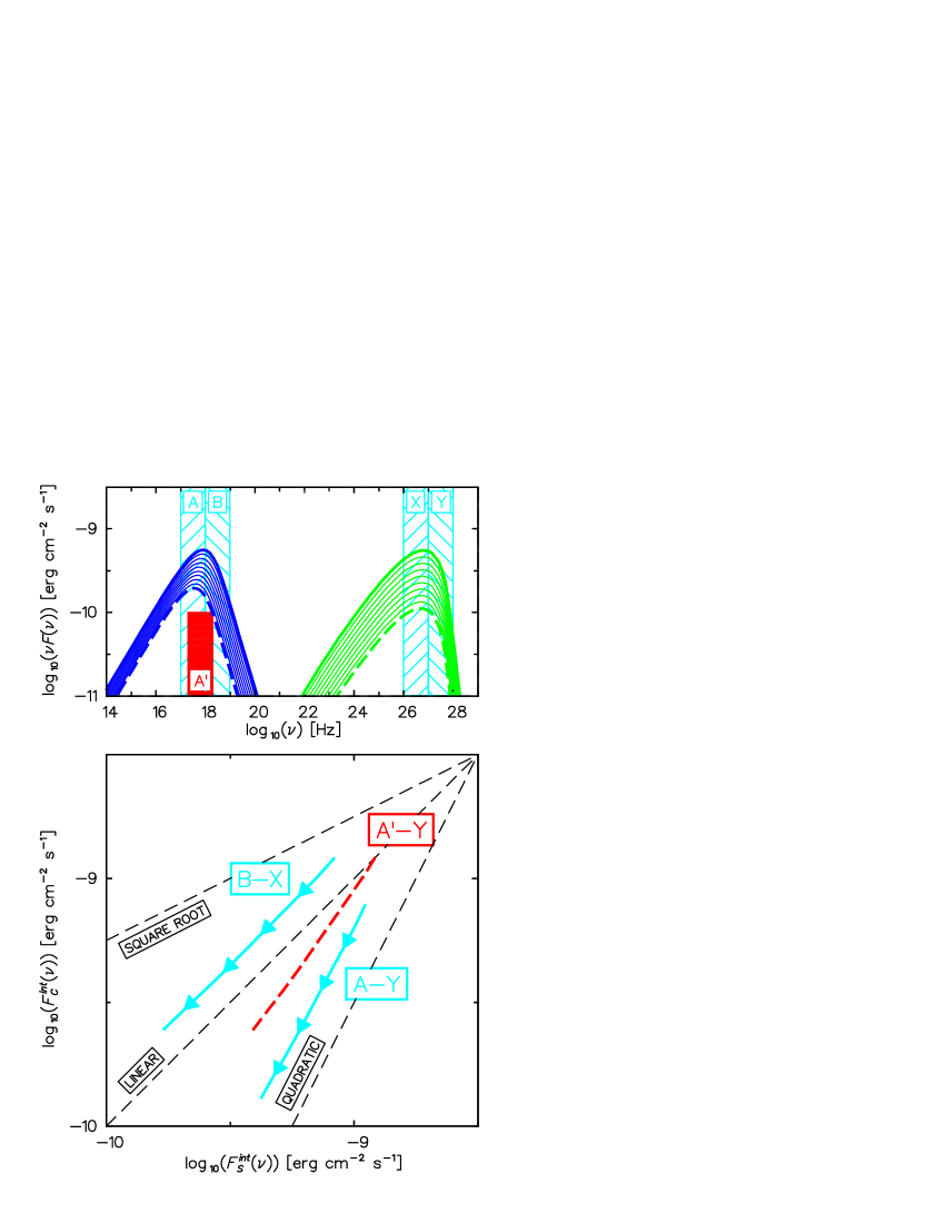
Figure 4: The upper panel shows the evolution of the SSC emission of an expanding spherical homogeneous source. The areas indicated by the capital letters show the spectral bands selected for the calculation of the correlation. The lower panel shows the two main correlations (bold solid lines with arrows which indicate the direction of the evolution) calculated for the evolutions presented in the upper panel. The bold dashed line in the lower panel (A’-Y) shows the correlation obtained after a small shift of the A–band. Thin dashed lines show a template for the correlations.

example of an evolving SSC spectrum during the expansion of homogeneous source. We use for this test the same set of physical parameters used for the numerical modeling presented in subsection 3.1. For each emission process we selected two spectral bands around the $\nu F(\nu)$ peak, named A ($10^{17}$–$10^{18}$ Hz), B ($10^{18}$–$10^{19}$ Hz) and X ($10^{26}$–$10^{27}$ Hz), Y ($10^{27}$–$10^{28}$ Hz). Note that most of the TeV emission is usually observed in our X–band. Some observations are still possible above the frequency $10^{27}$ Hz (see Figures 1-d and 2-d) in our Y–band but currently we are not able to obtain observations in the whole Y–band. However, the spectral index in the Y–band is relatively steep. Therefore, radiation observed in this band is dominated by the emission which comes from the low frequency part of this band which can be observed. In our test we calculate only two correlations for above described bands.

The first correlation (A–Y) is calculated between the evolution of the synchrotron emission (A) in a transition phase (from $F^{1}_{s}$ to $F^{2}_{s}$) and the evolution of the IC radiation (Y) in the Klein–Nishina regime ($F^{2}_{c}$). This gives an almost quadratic correlation. This particular correlation is a kind of transition between the correlation $c_{2}/s_{1}$ (3.4 for this particular test) and the correlation $c_{2}/s_{2}$ (which gives 1.214 for this particular case). The second correlation (B–X) is calculated between the evolution of the second part of the synchrotron radiation (B, $F^{2}_{s}$) and the evolution of the IC radiation (X) in a transition phase from the emission in the Thomson limit to the radiation in the Klein–Nishina regime. The correlation in this particular case is almost linear. This is the result of the transition from the correlation described by $c_{1}/s_{2}$ (equal to 0.786 in this particular case) and the correlation $c_{2}/s_{2}$ (equal 1.214 in this particular case).

The first test presented above shows that a quadratic correlation can be obtained in some specific cases when we observe the radiation emitted close to the $\nu F(\nu)$ peaks. However, we stress that this result depends strongly on the spectral bands used. This effect is clearly visible in Figure 4 where we show the correlation (A’–Y) after a small shift of the A–band (A’ $\to 2\times 10^{17}$–$2\times 10^{18}$ Hz). The almost quadratic correlation after this shift appears significantly less than quadratic. Moreover, to obtain the quadratic correlation we have assumed $m=1$. This means that the decrease of the magnetic field intensity was slower than we could expect from the rule which describes conservation of the magnetic flux ($m=2$).

3.6 Evolution of the $n_{2}$ parameter

In this subsection we analyse the effects related to the change of the index of the high energy electrons spectrum ($n_{2}$). The main reason for this test is to simulate the activity of Mrk 501 observed on April 1997. The observations obtained at that time by the $Beppo$SAX satellite (Fig. 1, Pian et. al. pian98 (1998)) indicate that the X–ray emission was almost stable around the energy 0.1 keV while the emission around 100 keV was very variable.

To simulate such evolution we change the value of the $n_{2}$ parameter in ten steps, assuming $n_{2}=2.5$ at the beginning of the simulation and increasing this value by a factor of 0.25 after each step. Note that the peak of the synchrotron spectrum, at the beginning of the test, is generated by the highest energy electrons ($\gamma_{\rm max}=10^{7}$, for this test) because $n_{2}<3$. The other model parameters are the same as in the previous modeling, except $\gamma_{\rm brk}$ which we changed to $3\times 10^{5}$ in order to obtain the constant emission around 0.1 keV energy. The radiative cooling is negligible for the physical parameters used in this simulation. In the next subsection we discuss in detail this phenomenon and we show that indeed this process is negligible.

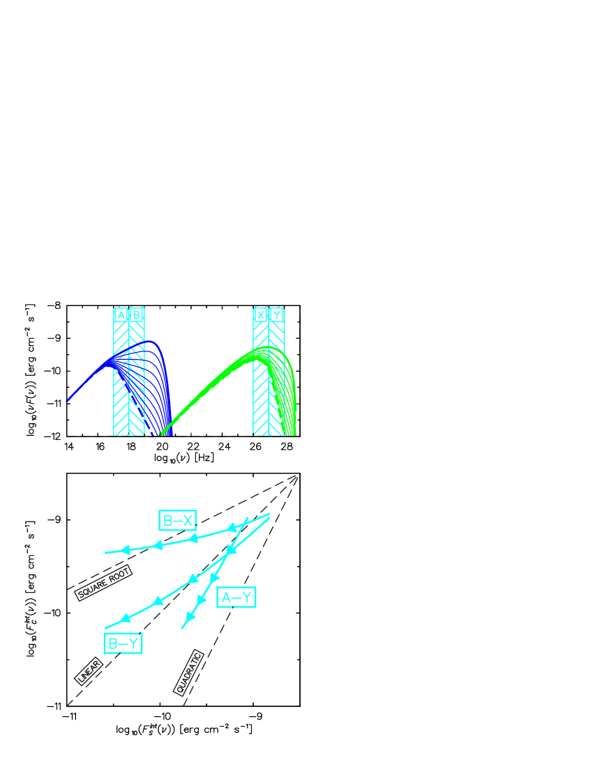
Figure 5: The upper panel shows the evolution of the SSC emission of the source where only the slope $n_{2}$ of the high energy part of the electron spectrum was modified during the simulation. To calculate the correlations presented in the lower panel we selected the same spectral bands as in the previous modeling. Thin lines in the lower panel show a template for the correlations.

In the test we selected the same spectral bands for the calculation of TeV/X–ray correlation as in the previous modeling and we also discus three different correlations. The first correlation (A-Y) is calculated selecting the TeV band decaying relatively fast and the part of the X–ray spectrum decreasing relatively slowly. At the beginning of the simulation the slope of the correlation is almost quadratic and becomes 1.7 towards the end of the simulation. In the second correlation (B-Y) we selected the parts of the TeV and X–ray spectra decreasing relatively fast. At the beginning of the simulation the two fluxes vary almost linearly. However, at the end of the simulation the correlation slope is close to 0.5. The third correlation (B-X) is opposite to the first relation (a fast decay of the X-rays with relatively slow decay of the TeV emission) and gives the slope close to 0.5 at the beginning of the simulation, changing rapidly and reaching the value of 0.13 at the end of the simulation.

This simulation can reproduce the activity of Mrk 501 observed in April 1997. The correlation between the Whipple and OSSE fluxes (Fig. 1) can be explained as the correlation between the spectral bands where the TeV and X–ray emission evolve relatively fast (e.g. the beginning of our correlation B-Y). The quadratic correlation between the Whipple and ASM fluxes can be explained as the correlation between the part of the TeV band which evolves relatively fast and the part of the X–ray emission which evolves relatively slowly (e.g. our correlation A-Y). However, the presented examples depend strongly on the position of the peaks and on the selected spectral bands.

3.7 Impact of the radiative cooling

In all the scenarios discussed so far we have assumed that the radiative cooling of the electrons is negligible. Now we assume that radiative cooling is important and we discuss its impact for the TeV/X–ray flux correlation.

To calculate the evolution of the electron energy spectrum including the radiative cooling we use the kinetic equation

$$\frac{\partial N^{*}(\gamma,t)}{\partial t}=\frac{\partial}{\partial\gamma}\left\{\left[C_{\rm cool}(t)\gamma^{2}+C_{\rm adia}(t)\gamma\right]N^{*}(\gamma,t)\right\},$$ (19)

where

$$C_{\rm cool}(t)=\frac{4}{3}\frac{\sigma_{T}}{m_{e}c}\left[U_{B}(t)+U_{\rm rad}(t)\right],\leavevmode\nobreak\ \leavevmode\nobreak\ \leavevmode\nobreak\ U_{B}(t)=\frac{B(t)^{2}}{8\pi}$$

describes the radiative cooling and $C_{\rm adia}=r_{a}/t$ describes the adiabatic cooling. For simplicity, we assume that the radiation field energy density ($U_{\rm rad}$) is equal to the magnetic field energy density ($U_{B}$). The initial distribution of the electron energy spectrum is given by a continuous broken power law

$$N_{0}(\gamma,t=t_{0})=k_{1}\gamma^{-n1}\left(1+\frac{\gamma}{\gamma^{0}_{\rm brk}}\right)^{n_{1}-n_{2}}.$$ (20)

The solution of this kinetic equation is given in Appendix B. However, this solution must be converted to a unit volume $N(\gamma,t)=N^{*}(\gamma,t),\left(t_{0}/t\right)^{3r_{e}}$ to be useful for the calculation of the emission coefficient (e.g. Kardashev kardashev62 (1962)). Since the evolution of the electron spectrum is quite complex, we use the numerical code to check the influence of the radiative cooling on the correlation.

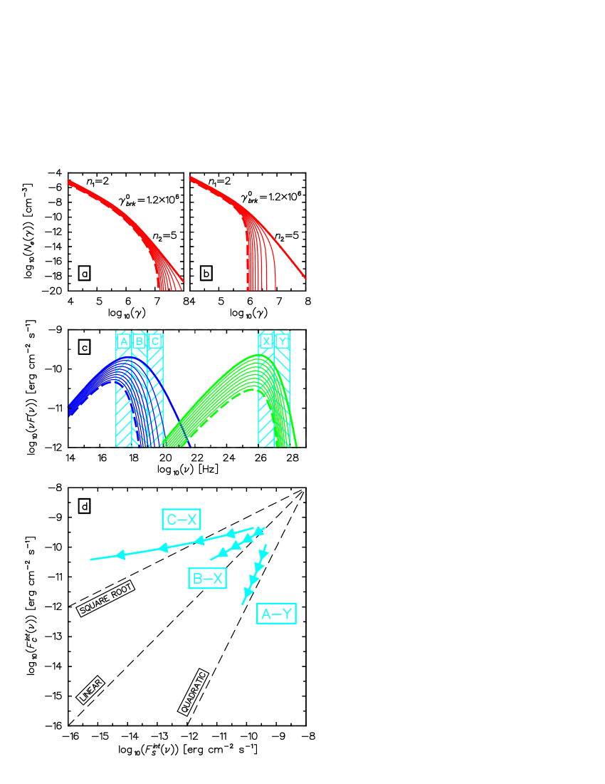
Figure 6: The impact of the radiative cooling for the correlation. Panel (a) shows the evolution of the high energy part of the electron energy spectrum for the physical parameters which we have selected for the modeling in the subsection 3.1. Panel (b) shows the evolution of the electrons spectrum for the parameters used in the subsection 3.7. The evolution of the synchrotron and the IC emission is shown in panel (c). We also show the spectral bands selected for the calculation of the correlations. Panel (d) shows three different correlations calculated for the tested evolution.

The radiative cooling may cause a fast decay of the high energy electrons. This appears as a cut–off in the high energy part of the electron spectrum. In Figure 6 we show two examples for the evolution of the spectrum. For the first assumed evolution (Fig. 6–a) the cooling is almost negligible while in the second example (Fig. 6–b) the cooling significantly modifies the high energy part of the electron spectrum. In the first test we use the same values of the physical parameters which we used for numerical calculations presented in the subsections 3.1, 3.5 and 3.6. In the second test we use significantly different values. We assume a larger initial intensity of the magnetic field ($B_{0}=0.004\to 0.02$ [G]) to increase the radiative cooling rate. We assume a smaller value of the Doppler factor ($\delta=50\to 30)$ and smaller initial source volume ($R_{0}=2\times 10^{16}\to 1.2\times 10^{16}$ [cm]) to keep the same level of the emission. Moreover, we also modify the initial density of the particles ($k_{1}=10^{3}\to 3\times 10^{3}$ [cm^-3]).

Figure 6–c shows the evolution of the synchrotron and the IC spectrum produced by the electron spectrum given in Figure 6–b. The cut–off in the electron spectrum produces an exponential decay of the synchrotron and the IC emission. Figure 6–c also shows the special bands selected for the calculation of the correlations. In this test we have introduced one more X–ray band (C, $10^{19}$ – $10^{20}$ [Hz]) to check the correlation when using the exponentially decaying part of the synchrotron emission.

The first correlation (A–Y), calculated for this test (Fig. 6–d), is analogous to the A–Y correlation computed neglecting radiative cooling. This is the correlation between the X–ray emission in the transition phase ($F^{1}_{s}\to F^{2}_{s}$) and the IC radiation in the Klein–Nishina regime. It gives, as in the previous test, an almost quadratic result. The second correlation B–X was calculated between the second part of the synchrotron emission ($F^{2}_{s}$) and the IC radiation in the Klein–Nishina regime ($F^{2}_{c}$, $c_{2}/s_{2}$). In principle this correlation should give a value of the correlation around 1.2 (see Table 1). However, the radiative cooling significantly modifies the evolution of the X–ray spectrum in the B–band. Thus, the X–ray emission decreases faster than in the evolution of the power law spectrum discussed in the previous subsection (see Figure 4). Therefore, we obtain an almost square root correlation in this case. The last correlation (C–X) is the most extreme case where we compare the evolution of the X–ray emission in the exponential decay part (C) with the evolution of the IC radiation in the Klein–Nishina regime ($F^{2}_{c}$). The exponential decay causes a very fast decrease of the synchrotron emission. Since this decrease is more than two times faster than the decrease of the IC radiation, the slope of the correlation is less than a square root.

The correlations presented in this subsection depend strongly on the position of the spectral bands. Moreover, the radiative cooling which causes the exponential decay of the spectra can destroy possible quadratic or linear correlations. This is related to the fact that the synchrotron emission responds immediately to the change of the high energy part of the electron spectrum while the relevant IC radiation is generated in the Klein–Nishina regime, mainly by the electrons with $\gamma$ less than $\gamma_{\rm brk}$ (see Figure 3-c-d). Moreover, the radiation field used in the scattering is not affected by the radiative cooling. To obtain almost quadratic result for the A-Y correlation we had to assume $m=1$.

4 Cylindrical source - pizza or spaghetti

So far we investigated the evolution of a spherical source. The geometry of the source is not important for the synchrotron emission as long as the electron self–absorption is neglected. On the other hand the geometry of the source may be very important for the IC emission which depends strongly on the radiation field available for the scattering. If the source is strongly extended in one dimension (e.g. $x$) then only the local radiation field, proportional to the other dimensions of the source ($y,z$), is important for the scattering. This effect is important for the observed correlation especially if the source expands in only one or two dimensions. To investigate this effect we approximate the emitting region by a cylindrical geometry, described by the radius ($R$) and the length ($L$) of the cylinder. We use this specific geometry to investigate two opposite cases. In the first case we assume $L\ll R$ a “pizza like” geometry (hereafter we call this the pizza case). In the second case we use the opposite assumption $L\gg R$ a “spaghetti like” geometry (hereafter we call this the spaghetti case).

The main reason for such assumptions is that we are looking for robust solutions which could explain a more than linear (or even quadratic) correlation during the decay of a flare. We also investigate when such solutions are independent of the specific spectral bands selected for the correlation. Using the cylindrical geometry we can simulate the expansion of the source in one dimension. This reduces the influence of the adiabatic cooling and the decay of the magnetic field. Moreover, with this geometry we can use a lower value of the Doppler factor (e.g. $\delta\sim 25$) and we are still able to avoid the impact of the radiative cooling ($B_{0}\sim 0.004$ [G]). In addition, for some specific viewing angles, we can neglect the light crossing time effect (e.g. a pizza–like source viewed face on, or a spaghetti–like source viewed at $1/\Gamma$, corresponding to a viewing angle of $90^{\circ}$ in the comoving frame).

We assume that the radius and the length of the cylindrical source evolve in time as power law functions

$$R(t)=R_{0}\left(\frac{t_{0}}{t}\right)^{-r_{e}},\leavevmode\nobreak\ \leavevmode\nobreak\ \leavevmode\nobreak\ \leavevmode\nobreak\ \leavevmode\nobreak\ L(t)=L_{0}\left(\frac{t_{0}}{t}\right)^{-l_{e}},$$ (21)

where $R_{0}$ and $L_{0}$ are initial radius and length respectively. This parameterization gives a volume which evolves in time as $V(t)=\pi R_{0}^{2}L_{0}\left(t_{0}/t\right)^{-E}$, where $E=(2r_{e}+l_{e})$.

The initial distribution of the electron energy spectrum is assumed to be a broken power law function as in the previous model (see Eq. 2). The evolution of the spectrum is given by a minimum of two power law functions as in the previous modeling (see Eq. 3). However, for this modeling the definition of the power law functions substituted for the minimum is different according to the different parameterization of the cylindrical geometry. The functions are given by the formulae

$$\begin{array}[]{ll}\vspace*{0.1cm}N_{1|2}(\gamma,t)=K_{1|2}(t)\gamma^{-n_{1|2}};&\leavevmode\nobreak\ \leavevmode\nobreak\ \leavevmode\nobreak\ \leavevmode\nobreak\ \leavevmode\nobreak\ K_{1|2}(t)=k_{1|2}\left(\frac{t_{0}}{t}\right)^{D}\left(\frac{t_{0}}{t}\right)^{A(n_{1|2}-1)},\\ \end{array}$$

where $D=(2r_{d}+l_{d})$ describes the evolution of the density and $A=(2r_{a}+l_{a})/3$ describes the adiabatic heating or cooling of the particles.

The evolution of the magnetic field intensity for this model is defined in the same way as in the previous modeling (see Eq. 1).

The evolution of the synchrotron emission coefficient is calculated for the low ($j^{1}_{s}$) and high energy electrons ($j^{2}_{s}$) separately

$$j^{1|2}_{s}(t)\propto K_{1|2}(t)B(t)^{\alpha_{1|2}+1}\propto k_{1|2}B_{1|2}\left(\frac{t_{0}}{t}\right)^{D+A(n_{1|2}-1)+m(\alpha_{1|2}+1)}.$$ (22)

The evolution of the intensity of the synchrotron emission is calculated along the source length

$$I^{1|2}_{s}(t)\propto L(t)j^{1|2}_{s}(t)\propto L_{0}k_{1|2}B_{1|2}\left(\frac{t_{0}}{t}\right)^{-l_{e}+D+A(n_{1|2}-1)+m(\alpha_{1|2}+1)},$$ (23)

If we assume that the observer is located outside the source at some distance on the symmetry axis of the cylinder then the observed flux is given by

$$\vspace*{0.1cm}F^{1|2}_{s}(t) \propto R^{2}(t)I^{1|2}_{s}(t)\leavevmode\nobreak\ \propto\leavevmode\nobreak\ R_{0}^{2}L_{0}k_{1|2}B_{1|2}\left(\frac{t_{0}}{t}\right)^{-s_{1|2}},$$ (24)

$$s_{1|2} = E-D-A(n_{1|2}-1)-m(\alpha_{1|2}+1).$$ (25)

The main difference between the previous modeling and the current calculations is in the IC emission. The difference comes from the energy density of the synchrotron emission ($U_{rad}$) which is available for the scattering.

First we describe the radiation in the pizza case where the evolution of the emission coefficient in the Thomson limit is defined by $j^{1}_{c_{p}}(t)\propto K_{1}(t)\leavevmode\nobreak\ I^{1}_{s}(t)$. The evolution of the IC emission coefficient for the Klein–Nishina regime is given by $j^{2}_{c_{p}}(t)\propto K_{2}(t)\leavevmode\nobreak\ I^{1}_{s}(t)$. In this particular pizza case we use for the calculation of the scattering only local radiation field that is proportional to the length of the source ($U_{rad}\propto I^{1}_{s}\propto j^{1}_{s}L$). We assume that the contribution of the synchrotron emission from the other parts of the source is negligibly small because the radiation field energy density decreases with the square of the distance. According to this assumption the radiation field used for the calculation of the IC scattering is isotropic. To obtain the evolution of the observed flux we have to multiply the evolution of the emission coefficient defined above by the source volume, which gives

$$\vspace*{0.1cm}F^{1}_{c_{p}}(t) \propto R_{0}^{2}L_{0}^{2}k^{2}_{1}B_{1}\left(\frac{t_{0}}{t}\right)^{-c_{1P}},$$ (26)

$$c_{1P} = 2r_{e}+2l_{e}-2D-2A(n_{1}-1)-m(\alpha_{1}+1),$$ (27)

for the Thomson limit and

$$\vspace*{0.1cm}F^{2}_{c_{p}}(t) \propto R_{0}^{2}L_{0}^{2}k_{1}k_{2}B_{1}\left(\frac{t_{0}}{t}\right)^{-c_{2P}},$$ (28)

$$\vspace*{0.1cm}c_{2P} = 2r_{e}+2l_{e}-2D-A(n_{1}-1)-A(n_{2}-1)$$ (29)

$$- m(\alpha_{1}+1),$$

for the Klein–Nishina regime.

In the spaghetti scenario we use only the local radiation field for the calculation of the scattering. However, now the local radiation field is proportional to the source radius ($U_{rad}\propto j^{1}_{s}R$). Therefore, the evolution of the emission coefficient in the Thomson limit is given by $j^{1}_{c_{s}}(t)\propto K_{1}(t)\leavevmode\nobreak\ R(t)\leavevmode\nobreak\ j^{1}_{s}(t)$. The evolution of this coefficient for the Klein–Nishina regime is defined by $j^{2}_{c_{s}}(t)\propto K_{2}(t)\leavevmode\nobreak\ R(t)\leavevmode\nobreak\ j^{1}_{s}(t)$. Finally, the evolution of the observed fluxes are calculated in the same way as in the pizza scenario. For the Thomson limit we have

$$\vspace*{0.1cm}F^{1}_{c_{s}}(t) \propto R_{0}^{3}L_{0}k^{2}_{1}B_{1}\left(\frac{t_{0}}{t}\right)^{-c_{1S}},$$ (30)

$$c_{1S} = 3r_{e}+l_{e}-2D-2A(n_{1}-1)-m(\alpha_{1}+1),$$ (31)

and for the Klein–Nishina regime we have

$$\vspace*{0.1cm}F^{2}_{c_{s}}(t) \propto R_{0}^{3}L_{0}k_{1}k_{2}B_{1}\left(\frac{t_{0}}{t}\right)^{-c_{2S}},$$ (32)

$$\vspace*{0.1cm}c_{2S} = 3r_{e}+l_{e}-2D-A(n_{1}-1)-A(n_{2}-1)$$ (33)

$$- m(\alpha_{1}+1).$$

4.1 Specific solutions

With respect to the spherical geometry, the cylinder is parametrized by two more free parameters ($L_{0}$, $l_{e}$) which give more possible scenarios for the time evolution of the flux. In this subsection we discuss only a few possible cases that give directly a quadratic correlation between the second part of the synchrotron emission ($F^{2}_{s},s_{2}$) and the IC radiation in the Klein–Nishina regime ($F^{2}_{c},c_{2}$) during the decay of a flare.

• Consider a pizza–like geometry and only linear increase of the source length ($l_{e}=1$, $r_{e}=r_{d}=r_{a}=l_{d}=l_{a}=m=0$). The increase causes a linear growth of the synchrotron emission ($F^{1|2}_{s}\propto t^{l_{e}},s_{1|2}=1$) and a quadratic ($c_{(1|2)P}=2$) increase of IC radiation which is proportional to the increase of the volume and the radiation field as well ($U_{rad}\propto j_{s}L\propto t^{l_{e}}$). Thus in all possible cases we can obtain the quadratic correlation ($c_{(1|2)P}/s_{1|2}=2$). The same test for the spaghetti case gives $c_{(1|2)P}/s_{1|2}=1$ because the local radiation field is proportional to the radius and is constant. Note that the similar test for the spherical geometry ($r_{e}=1,r_{d}=r_{a}=m=0$) gives $c_{1|2}/s_{1|2}=1.333$.

• In the next test we assume a pizza–like geometry with expansion of the radius, decrease of the density and the adiabatic losses that correspond to the change of the radius ($r_{e}=r_{d}=r_{a}=1$). The other parameters are assumed to be constant ($l_{e}=l_{d}=l_{a}=m=0$). For $r_{e}=r_{d}$ the expansion of the volume is compensated entirely by the decrease of the density. Therefore, the synchrotron emission decreases only due to the adiabatic cooling ($F^{2}_{s}\propto t^{-2r_{a}(n_{2}-1)/3},s_{2}=2.67$). The IC emission in the Klein–Nishina regime depends on the expanding volume ($t^{2r_{e}=2}$), the square of the decreasing density ($t^{-4r_{d}=-4}$) and the adiabatic losses of the low and high energy electrons ($t^{-2r_{a}(n_{1|2}-1)/3=-(0.67|2.67)}$). The combination of the above processes gives a decrease $F^{2}_{c}\propto t^{-5.33}$, which finally provides a quadratic correlation ($c_{2P}/s_{2}=2$). However, the correlation depends on the value of the $n_{1}$ and $n_{2}$ parameter ($n_{1|2}=2|5$, in the above test). We have checked that for a given value of the parameter $n_{1}$ in the range from 1.5 to 2.5 there is always only one value of the index $n_{2}$ which provides the quadratic result (e.g. $n_{1}=2.5$ and $n_{2}=5.5$). Other correlations for this case, which we do not discuss in detail, are described by $c_{1P}/s_{1}=5$, $c_{1P}/s_{2}=1.25$, $c_{2P}/s_{1}=8$.

• The quadratic correlation can be obtained also in a three dimensional expansion of a pizza–like source ($r_{e}=r_{d}=r_{a}=l_{e}=l_{d}=l_{a}=1$). However, to get the quadratic result it is necessary to assume a constant magnetic field ($m=0$) during the expansion and specific values of the parameters $n_{1}$ and $n_{2}$ (e.g. $n_{1}=2$ and $n_{2}=4$). Note that similar three dimensional expansion of the spherical source ($r_{e}=1=r_{d}=r_{a}=1,m=0$) gives $c_{2}/s_{2}=1.75$.

• The spaghetti scenario also provides a quadratic correlation if we assume the expansion of the radius and the length of the source ($r_{e}=r_{d}=r_{a}=l_{e}=l_{d}=l_{a}=1$). However, also in this case we have to assume a constant magnetic field ($m=0$) and specific slopes of the electron spectrum (e.g. $n_{1}=2$ and $n_{2}=4$) to get the right correlation.

We conclude that the cylindrical geometry can provide some quadratic solutions if we can assume a constant or almost constant value of the magnetic field during the evolution of the source. Moreover, we have also to assume that the impact of the radiative cooling is negligible. Otherwise with this particular geometry the explanation of the quadratic result of the correlation $c_{2}/s_{2}$ is rather problematic.

5 Light crossing time effects (LCTE)

We distinguish two different types of LCTE. The first effect, which we call the internal LCTE, is important for the calculation of the evolution of the radiation field inside the source. This effect is especially important for precise calculation of the IC emission. The second effect, which we call the external LCTE, is important for the observer. We investigate in detail in this subsection this second effect, which seems to have a stronger impact for the correlation between the TeV and X–ray emission. Note that recently Sokolov, Marscher & McHardy (sokolov04 (2004)) proposed a new model to explain the rapid multifrequency variability of blazars. They investigated in detail the influence of LCTE for the observed emission. This model provide especially precise description of the IC scattering in a case where the internal LCTE is important.

To check the influence of the external LCTE for the correlation we have used the model proposed by Chiaberge $\&$ Ghisellini (chiaberge99 (1999)). They assumed that the source is created by a shock wave which accelerates the electrons. The electrons are injected from the shock region into a volume of the jet where they generate most of the synchrotron and the IC radiation. The geometry of the emitting region is approximated to be cubic and the region has been divided into small homogeneous cells. In figure 7 we sketch the evolution of such a source. On the right we show the intrinsic evolution. On the left we show the evolution of the part of the source that can be observed in the comoving frame at $90^{\circ}$ with respect to the shock velocity. The number in each cell indicates the age of the particles inside the cell.

If the external LCTE is not important then the observer can see immediately the changes of the total source structure. This condition is true for this model if the shock velocity ($\beta_{s}$) is significantly less than the speed of light. Otherwise only part of the source volume can be observed by the observer at given time.

We examine two theoretical scenarios of the source evolution. In the first we assume that the emission of a single cell is constant in time. For the second scenario, opposite to the previous one, we assume a very fast flux decay within a single cell.

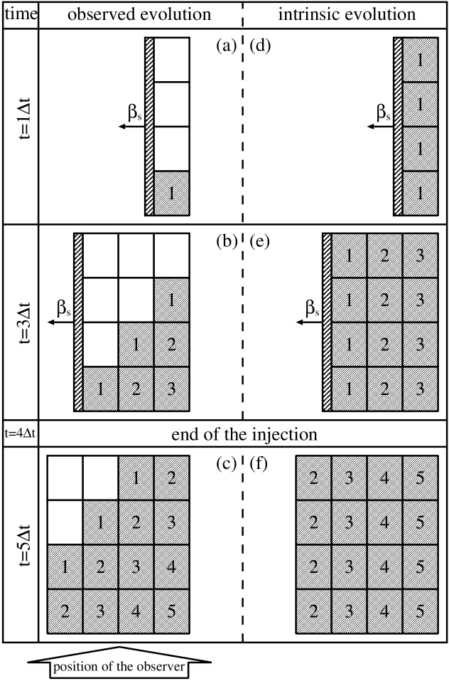
Figure 7: The evolution of the source according to the model proposed by Chiaberge $\&$ Ghisellini (chiaberge99 (1999)). The right column shows evolution of the total volume of the source. The left column shows the cells that contribute to the source emission observed at given time by the observer located at $90^{\circ}$ (bottom of the figure) with respect to the shock velocity ($\beta_{s}$) in the comoving frame. The number in each cell indicates the age of the particles. Note that at time $4\Delta t$ the injection process was stopped.

5.1 Constant emission of a single cell

The assumption of constant emission requires the same age of the particles in all cells. This means that in cell presented in Figure 7 we should have the same number–1. To check the influence of the process for the evolution of the emission we compare the intrinsic evolution of the source with the observed evolution.

For the intrinsic evolution of the source the constant injection of the cells gives a linear increase of the synchrotron emission, which is proportional to the increase of the source volume. If we neglect the internal LCTE, the IC radiation also will increase proportionally to the increase of the volume. However, this assumption is not precise and we will discuss the problem of the internal LCTE at the end of this section. Immediately after the the injection stops (for example due to destruction of the shock wave) we should observe a constant emission of the source where the absolute level of the emission is proportional to the created volume.

If we consider the external LCTE then observer at the beginning of the evolution ($t=\Delta t$) will receive only the emission from the cell which is nearest to him (bottom row of the cells). At a later time the observer will start to receive successively emission produced by the cells located at larger distances. If the emission of a single cell is constant in time (number 1 in all observed cells) then the observed emission increases as a sum

$$\sum_{k=1}^{n}k=\frac{n(n+1)}{2},$$ (34)

where $n$ is the number of cells in the bottom row. Note that this formula is correct only for the source which at the end of the injection is a square ($n\times n$ cells) and is correct only for the injection phase. This simple estimation indicates that the observed flux will increase in time as $t^{\sim 2}$ if $n\gg 10$. This result is significantly different from the intrinsic evolution where the increase of the emission in the injection phase was linear. Therefore, this simple test shows that the external LCTE may significantly change the evolution of the observed emission. Note that in this test the level of the emission increases also after the end of the injection. However, in this phase the increase is slower than $t^{\sim 2}$ and after some time ($2\times l/c$ where $l$ is the dimension of the square source) the flux level becomes constant, and equal to the level of the intrinsic emission after the end of the injection.

5.2 Very fast decay of a single cell

We now assume that the flux, within a single cell, decays very fast. The “life time” of a single cell is $\Delta t$.

If the external LCTE is not important we observe constant emission of the source as long as the shock is injecting particles. The total volume of the source during the whole injection process is represented only by the cells next to the shock front (e.g. Figure 7-d). The source disappears abruptly after the end of the injection.

When the external LCTE is important, at the beginning of the injection the observer will see only the radiation produced by the bottom row, reduced in this particular case to a single cell. At a later time the radiation produced by the cells at larger distances will arrive at the observer. This means that the observer will see a linear increase of the emission. The duration of this increase depends on the number of cells ($k$) in the column next to the shock front. After the time $k\times\Delta t$ the observed emission should be constant.

After the end of the injection we should observe a linear decrease of the emission with a duration equal to the light crossing time from the back to the near part of the source. This is the opposite behavior to the linear increase observed at the beginning of the simulation.

There are two important conclusions from this test. The first is that even if the intrinsic emission of the source is constant for some time at the beginning of the evolution, the observer will see a linear increase of the radiation. The second conclusion concerns the decay of the source. Even if the source “dies” abruptly in a very short time, the observer will see a linear decay of the emission for a time corresponding to the dimension of the source. The conclusions obtained in this and in the previous subsection are strictly valid for the specific adopted geometry. In the next subsection we discuss more possible implications of LCTE.

5.3 LCTE - general conclusions

The model used to explore the influence of LCTE for the evolution of the source emission gives the possibility to investigate only the external LCTE. However, the conclusion obtained from the simple test which we have performed with this model seems to be quite strong. If the emission produced by the total volume of the source evolves in time as $t^{x}$ then the observed emission evolves as $t^{x+1}$. Besides being confirmed by our simple analytical tests, this very simple rule is also confirmed by numerical calculations assuming several different decay rates of a single cell emission. However, this result is strictly valid only for the proposed geometry, source evolution and specific position of the observer (at $90^{\circ}$). The model used cannot precisely describe the evolution of the radiation field inside the source (internal LCTE) and cannot describe the emission of the expanding source. This would require a more sophisticated numerical modeling.

If we assume that the external LCTE indeed increases by one the index which describes the evolution of the emission, then we can analyze the impact of this process for the observed correlation. If for example the correlation between the synchrotron and the IC emission is intrinsically quadratic then the observed correlation will not be quadratic. This is a simple consequence of the rule already discussed in subsection 3.3 (if $c/s=2$ then $(c+x)/(s+x)\neq 2$). On the other hand if we observe a quadratic correlation it means that the intrinsic change of the IC emission must be much larger that the change of the synchrotron radiation. For example we need $F_{s}\propto t^{s=1}$ and $F_{c}\propto t^{s=3}$ intrinsically to obtain a quadratic correlation after the basic transformation due to the external LCTE ($(c=3+1)/(s=1+1)=2$). The transformation indicates that only some specific intrinsic evolutions of the synchrotron and the IC emission (e.g. $c=1\leavevmode\nobreak\ \&\leavevmode\nobreak\ s=0$, $c=3\leavevmode\nobreak\ \&\leavevmode\nobreak\ s=1$, $c=5\leavevmode\nobreak\ \&\leavevmode\nobreak\ s=2$) may provide a quadratic correlation. Similar arguments apply to any observed correlation slope.

The significantly faster evolution of the intrinsic IC flux with respect to the evolution of the intrinsic synchrotron flux seems difficult to explain. If we neglect the internal LCTE, then for the calculation of the IC scattering inside a single cell we use only the synchrotron radiation field produced within this cell. With this assumption the evolution of the IC and synchrotron radiation will be exactly the same ($c=s$). However this approach is of course not always exact, since electrons inside a given cell may scatter the seed photons produced also by the surrounding cells. The cell at the center of the source is the one most affected by this effect. For such a cell we could have a linear increase of the radiation field during the injection phase. The cells affected the least will be the ones at the corners of the source (for them the effect should be four times less than for the cell in the center). Therefore, the evolution of the intrinsic IC emission of the whole source should be more than linear but less than quadratic ($F_{c}\propto t^{1\leavevmode\nobreak\ <\leavevmode\nobreak\ c\leavevmode\nobreak\ <\leavevmode\nobreak\ 2}$) which after the transformation gives $2<c<3$. This estimation requires constant intrinsic synchrotron emission to explain a quadratic correlation in the observer frame.

To conclude: i) if the intrinsic evolution of the source produces a given correlation between the synchrotron and IC emission, then the external LCTE yields a correlation with a different slope; ii) if we observe a given correlation and the external LCTE is important, then the intrinsic relative IC/synchrotron change must be much stronger than what is observed.

6 Summary and conclusions

We have presented a detailed study of the expected correlation between the variations observed in the X-ray and TeV bands in HBL, in the context of the widely-used homogeneous SSC model. This work has been stimulated by the observations of both linear and quadratic correlations in the few cases for which the available data are suitable for a detailed study of the correlation in single flaring events (Section 2).

First we addressed the problem in the context of the widely used spherical geometry (Section 3), presenting analytical relations valid when the radiative cooling can be neglected and numerical results valid in general. While a quadratic correlation during the increasing phase of a flare is easy to reproduce through an increase in the density (due, for instance, to a continuous injection of new particles in the emitting volume), we found that the same correlation observed during the decreasing phase poses a difficult problem. A case close to a quadratic relation can be obtained only in the rather physically implausible case of adiabatic expansion and a constant magnetic field. When the observational bands comprise the peaks of the SEDs the situation is more complex even if a close-to-quadratic relation can be obtained, the solution strongly depends on the exact position of the bands and a small change in the observational limits inevitably would change the correlation.

The main conclusion that we can derive from the first part of our study is that in order to to get a quadratic (or, even more general, more-than-linear) correlation between X-rays and TeV we need rather special conditions and/or fine-tuning in the temporal evolution of the physical parameters. For special choices of the spectral bands under study and of the parameters describing the evolution we can get even more-than-quadratic relations. In all the cases these solutions are quite “delicate” a small change in the observational band and/or in the parameters inevitably changes the correlation.

Next (Section 4) we investigated the changes related to a source geometry, assuming that the emitting region is a cylinder. Synchrotron emission is not affected by the actual shape of the emission region (as long as absorption effects within the source are negligible). On the other hand the value of the radiation energy density strongly depends on the geometry, affecting the SSC emission. We distinguish between two cases (called pizza or spaghetti) depending on the ratio between the length and radius of the cylinder ($R/L>1$ or $R/L<1$ respectively). We found that, similar to the spherical case, quadratic solution can be found only assuming that the magnetic field is not affected by the expansion. Moreover, radiative cooling can destroy the correlation.

Although light crossing time effects have not been directly taken into account in the calculations, we have briefly discussed possible effects of this phenomena (Section 5). We show that the external LCTE can “weaken” the intrinsic (within the source) correlation. On the other hand if we observe for example a quadratic correlation and the external LCTE is important then the intrinsic IC/synchrotron change must be stronger than quadratic (e.g. $c/s=3/1$).

As a last step we discussed the possibility that the SSC occurs in the Thomson regime. This would easily produce a quadratic correlation between X-rays and TeV, since the seed photons for the IC scattering are produced by the same electrons. However this would require rather implausible conditions for the emission region (extreme Doppler factors, $\delta\sim 1000$, and an extremely compact source, see Appendix A).

The general conclusion is that if the quadratic correlation during single flares will be found to be common, the simple homogeneous SSC model will face a severe problem. As stressed many times, the main difficulty is to explain the decaying phase, therefore acceleration processes and/or particular injection mechanisms cannot contribute to solving the problem.

Appendix A Large Doppler factor – the Thomson limit

The main difficulty in explaining a more than linear correlation between the TeV and the X–ray fluxes is associated with the fact that in TeV sources the seed photons to be scattered at high energies are those below the peak of the synchrotron emission, because the Klein–Nishina decline of the scattering cross section with energy implies a small efficiency for the scattering between photons at the synchrotron peak and electrons with random Lorentz factor close to $\gamma_{\rm brk}$. This “decoupling” between scattering electrons and scattered seed photons introduces the problems we have discussed.

Indeed, Tavecchio et al. (tavecchio98 (1998)) have demonstrated that in the single zone, homogeneous SSC model, the knowledge of the peak frequencies $\nu_{s}$ and $\nu_{c}$, the flux at these frequencies, and the variability timescale is sufficient to determine the physical parameters of the source. In this case one associates the variability timescales $t_{\rm var}$ with the size $R$ of the source, through $R=ct_{\rm var}\delta$. Application to Mrk 421 and Mrk 501 using this prescription results in the finding that both sources are suffering from Klein–Nishina effects.

We now relax the assumption $R=ct_{\rm var}\delta$, and require instead that the scattering of X–ray photons with the electrons producing these same photons (by the synchrotron process) occurs in the Thomson limit. This will have the advantage that any variations of the number of electrons emitting in the X–ray band will automatically produce a quadratic variation in the TeV band.

To this aim we define $\gamma_{x}$ as the random Lorentz factor of those electrons producing synchrotron photons of frequency $\nu_{x}$, and require (Thomson limit)

$${h\nu_{x}\over m_{e}c^{2}}\,{\gamma_{x}\over\delta}\,<\,1$$ (35)

Since $\nu_{x}\simeq 3.6\times 10^{6}B\gamma_{x}^{2}\delta$, the above condition yields

$$B\delta^{3}\,>\,\left({h\over m_{e}c^{2}}\right)^{2}\,{\nu_{x}^{3}\over 3.6\times 10^{6}}$$ (36)

If the scattering occurs mainly in the Thomson limit, then the ratio between the self Compton and the synchrotron peak frequencies is $\nu_{c}/\nu_{s}=(4/3)\gamma_{\rm brk}^{2}$. Since the synchrotron peak frequency is given by $\nu_{s}\simeq 3.6\times 10^{6}B\gamma_{\rm brk}^{2}\delta$, we have

$$B\delta\,=\,{\nu_{s}^{2}\over 2.8\times 10^{6}\nu_{c}}$$ (37)

The third condition concerns the synchrotron and self Compton peak fluxes. The intrinsic (comoving) synchrotron radiation energy density is given by $U^{\prime}_{\rm syn}\,=\,{L_{\rm syn}/4\pi R^{2}c\delta^{4}}$. Since, in the Thomson regime, we have $L_{c}/L_{s}=U^{\prime}_{\rm syn}/U_{B}$, we have the third requirement

$$B\delta^{2}R\,=\,\left({2L_{\rm syn}^{2}\over cL_{c}}\right)^{1/2}$$ (38)

Equations 36, 37 and 38 form a closed system of equations in the unknowns $B$, $\delta$ and $R$. The solutions are

$$\delta\,=\,\left({a\over b}\right)^{1/2};\leavevmode\nobreak\ \leavevmode\nobreak\ \leavevmode\nobreak\ \leavevmode\nobreak\ \leavevmode\nobreak\ B\,=\,{b^{3/2}\over a^{1/2}};\leavevmode\nobreak\ \leavevmode\nobreak\ \leavevmode\nobreak\ \leavevmode\nobreak\ \leavevmode\nobreak\ R\,=\,\left({2L_{\rm syn}^{2}\over cL_{c}}\right)^{1/2}{1\over(ab)^{1/2}}$$ (39)

where

$$a\,\equiv\,\left({h\over m_{e}c^{2}}\right)^{2}\,{\nu_{x}^{3}\over 3.6\times 10^{6}};\qquad b\,\equiv\,{\nu_{x}^{2}\over 2.8\times 10^{6}\nu_{c}}$$ (40)

For illustration, consider the case $\nu_{s}=1$ keV, $\nu_{c}=0.5$ TeV, $\nu_{x}=$ 10 keV, and equal synchrotron and self Compton luminosities, $L_{\rm syn}=L_{c}=10^{45}$ erg s^-1. Then we obtain $B=0.14$ G, $\delta=1200$ and $R=1.2\times 10^{12}$ cm. With these parameters, the cooling frequency after one hour (observed time) is of the order of $5\times 10^{16}$ Hz. The minimum variability timescale, fixed by the light crossing time, is $t_{\rm var}\sim R/c\delta\simeq 0.03$ s. As we can see, the required beaming factor is rather extreme for this reason we consider this solution very unlikely.

Appendix B Solution of the kinetic equation

Analytical solution of the kinetic equation used in subsection 3.7 is given by following formula

$$N^{*}_{e}(\gamma,t) = \left[k_{1}\{S_{1}(\gamma,t)/\gamma\}^{n_{1}}S_{2}(\gamma,t)\left(1+\frac{\gamma}{S_{1}(\gamma,t)\gamma^{0}_{\rm brk}}\right)^{n_{1}-n_{2}}\right],$$ (41)

$$S_{1}(\gamma,t) = [I_{1}(t)-\gamma I_{2}(t)],$$

$$S_{2}(\gamma,t) = \exp\Bigg{[}-\int^{t}_{t_{0}}\Big{\{}\gamma C_{\rm adia}(t^{\prime})I_{2}(t)-\gamma C_{\rm adia}(t^{\prime})I_{2}(t^{\prime})$$

$$- C_{\rm adia}(t^{\prime})I_{1}(t)-2\gamma I_{1}(t^{\prime})C_{\rm cool}(t^{\prime})\Big{\}}$$

$$\Big{/} \Big{\{}\gamma I_{2}(t^{\prime})-\gamma I_{2}(t)+I_{1}(t)\Big{\}}\mathrm{d}t^{\prime}\Bigg{]},$$

$$I_{1}(x) = \exp\left[-\int_{t_{0}}^{x}C_{\rm adia}(y)\mathrm{d}y\right],\leavevmode\nobreak\ \leavevmode\nobreak\ \leavevmode\nobreak\ \leavevmode\nobreak\ I_{2}(x)=\int_{t_{0}}^{x}C_{\rm cool}(y)I_{1}(y)\mathrm{d}y,$$

This solution describes evolution of the electron energy spectrum only for the case where the initial spectrum is approximated by the continuous broken power law function (Eq. 20).

References

- (1) Aharonian, F., A., 2000, New Astronomy, 5, 377
- (2) Atoyan, M., A., & Aharonian, F., A., 1999, MNRAS, 302, 253
- (3) Bednarek, W., Protheroe, R., J., 1997, MNRAS, 292, 646
- (4) Begelman, M. C., Rees, M. J., & Sikora, M., 1994, ApJ, 429, L57
- (5) Buckley, J., H., et al. 1996, ApJ, 472, L9
- (6) Böttcher, M., 2004, NewAR, 8, 399
- (7) Böttcher, M., & Dermer, C., D., 2002 ApJ, 564, 86
- (8) Catanese, M., Bradbury, S., M., Breslin, A., C., et al. 1997, ApJ , 487, L143
- (9) Chiaberge, M., Ghisellini, G., 1999, MNRAS , 306, 551
- (10) Dermer C.D., Schlickeiser R., 1993, ApJ , 416, 458
- (11) Djannati–Atai, A., Piron, F., Barrau, A., et al., 1999, AA, 350, 17
- (12) Dondi, L., & Ghisellini, G., 1995, MNRAS, 273, 583
- (13) Edwards, P., G., & Piner, B., G., 2002, ApJ, 579, L70
- (14) Fossati, G., Buckley, J., Edelson, R., A., et al., 2004, NewAR, 48, 419F (Proceedings of the 2nd Veritas Symposium, April 2003, Chicago)
- (15) Georganopoulos, M., & Kazanas, D., 2003, ApJ, 594L, 27
- (16) Ghisellini, G., Celotti, A., & Costamante, L., 2002, A&A, 386, 833
- (17) Giroletti, M., Giovannini, G., Feretti, L. et al., 2004, ApJ, 600, 127
- (18) Gould, R., J., 1979, AA, 76, 306
- (19) Guetta, D., Ghisellini, G., Lazzati, D., Celotti, A., 2004, AA, 421, 877
- (20) Kardashev, N., S., 1962, Soviet Astronomy–AJ, 6, 317
- (21) Kino, M., Takahara, F., & Kusunose, M., 2002, ApJ, 564, 97
- (22) Kirk, J. G., Rieger, F. M., Mastichiadis, A., 1998, A&A, 333, 452
- (23) Konopelko, K., Mastichiadis, A., Kirk, J., et al. 2003, ApJ, 597, 851
- (24) Katarzyński, K., Sol, H., & Kus, A., 2001, AA, 367, 809
- (25) Katarzyński, K., Sol, H., & Kus, A., 2003, A&A, 410, 101
- (26) Krawczynski, H., Coppi, P., S., Maccarone, T., et al., 2000, AA, 353, 97
- (27) Krawczynski, H., Sambruna, R., Kohnle, A., et al., 2001, ApJ, 559, 187
- (28) Krawczynski, H., Coppi, P., & Aharonian, F., 2002, MNRAS, 336, 721
- (29) Krawczynski, H., Hughes, S., Horan, D., et al., 2004, ApJ, 601, 151
- (30) Krawczynski, H., 2004, NewAR, 48, 367
- (31) Longair, S., M., 1992, V1 p340, High Energy Astrophysics (Cambridge University Press, UK)
- (32) Mannheim, K., 1993, A&A, 269, 67
- (33) Maraschi, L., Fossati, G., Tavecchio, F., et al., 1999, ApJ , 526, L81
- (34) Mastichiadis, A., & Kirk, J., 1997, A&A, 320, 19
- (35) Moderski, R., Sikora, M., & Blazejowski, M., 2003, A&A, 406, 855
- (36) Mücke, A., et. al. 2003, Astropart. Phys., 18, 593
- (37) Pian, E., Vacanti, G., Tagliaferri, G., et al., 1998, ApJ, 492, L17
- (38) Piner, B., G., Unwin, S., C., Wehrle, A., E., et. al., 1999, AAS, 194, 5030
- (39) Piner, B., G., & Edwards, P., G., 2004, ApJ, 600, 115
- (40) Pohl, M. & Schlickeiser, R., 2000, A&A, 354, 395
- (41) Punch, M., Akerlof, C., W., Cawley, M., F., et al., 1992, Nature, 358, 477P
- (42) Rees, M., J., 1978, MNRAS, 184, P61
- (43) Rybicki, G., Lightman, A., P., 1979, Radiative Processes in Astrophysics, Wiley Interscience, New York
- (44) Sokolov, A., Marscher, A., P., & McHardy, I., M., 2004, astro-ph 0406235
- (45) Takahashi, T., Kataoka, J., Madejski, G., et al., 2000, ApJ, 542, 105
- (46) Tanihata, C., Kataoka, J., Takahashi, T., et at., 2004, ApJ, 601, 759
- (47) Tavecchio, F., Maraschi, L., Pian, E., et al., 2001, ApJ, 554, 725
- (48) Tavecchio, F., Maraschi, L., & Ghisellini, G., 1998, ApJ, 509, 608