Can one hear the shape of the Universe?

Abstract

It is shown that the recent observations of NASA’s explorer mission “Wilkinson Microwave Anisotropy Probe” (WMAP) hint that our Universe may possess a non-trivial topology. As an example we discuss the Picard space which is stretched out into an infinitely long horn but with finite volume.

When Einstein wrote his seminal paper of 1917 Einstein_1917 which laid the foundation of modern cosmology, he believed that the global geometry of our Universe, i. e. the spatial curvature, the topology and thus its shape, are determined by the theory of general relativity. However, since the Einstein gravitational field equations are differential equations, they only constrain the local properties of space-time but not the global structure of the Universe at large. In the concordance model of cosmology our Universe is at large scales spatially flat and possesses the trivial topology, implying that it has infinite volume. It is remarkable that already in 1900 Schwarzschild pointed out Schwarzschild_1900 that the geometry of the three-dimensional space of astronomy might be non-Euclidean and that there is the possibility of spaces with non-trivial topology (Clifford-Klein space forms) which do not necessarily lead to infinite universes as commonly believed.

Already in 1992, COBE Smoot_et_al_1992 discovered the temperature fluctuations $\delta T$ of the cosmic microwave background radiation (CMB) and, in particular, detected in the angular power spectrum a strange suppression of the quadrupole moment. The first-year WMAP data Bennett_et_al_2003 confirm COBE’s measurements. The temperature correlation function $C(\vartheta)=\left<\delta T(\hat{n})\,\delta T(\hat{n}^{\prime})\right>$ displays very weak correlations at wide angles Hinshaw_et_al_1996 ; Bennett_et_al_2003 , $70^{\circ}\lesssim\vartheta\lesssim 150^{\circ}$, see the solid curve in Fig. 1. (Here $\hat{n},\hat{n}^{\prime}$ denote unit vectors in the directions from which the photons arrive; $\hat{n}\cdot\hat{n}^{\prime}=\cos\vartheta$.) Fig. 1 also shows as a dotted curve the theoretical prediction according to the concordance model ($\Lambda$CDM) using the best-fit values for the cosmological parameters as obtained by WMAP Bennett_et_al_2003 . The shaded region represents the $1\sigma$ deviations which are obtained from 3000 simulations by HEALPixGorski_Hivon_Wandelt_1999 .

It is seen that the concordance model does not reproduce the experimentally observed suppression of power at wide angles as emphasized by the WMAP team Bennett_et_al_2003 ; Spergel_et_al_2003 . For the $S$ statistic, $S(\alpha):=\int_{-1}^{\cos\alpha}|C(\vartheta)|^{2}d\cos\vartheta$, which quantifies the lack of power on large scales, it is found Spergel_et_al_2003 for $\alpha=60^{\circ}$ that only 0.15% of 100 000 Monte Carlo simulations have lower values of $S$. A quadratic maximum likelihood analysis gives, however, somewhat larger probabilities in the range 3.2-12.5% Efstathiou_2004 . The temperature spectrum is directly linked with the polarization spectrum by the local quadrupole at the onset of reionization. Skordis and Silk take this into account and find that the probability that the quadrupole is as low as or lower than $250(\mu\text{K})^{2}$, is reduced to an order of $10^{-4}$ Skordis_Silk_2004 . We shall argue that the large power of the concordance model on large scales is due to the infinite volume of the considered flat model for the universe.

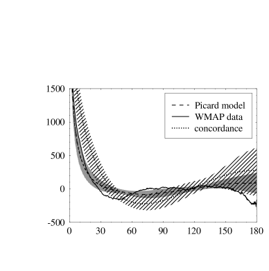
Figure 1: The mean temperature correlation function $C(\vartheta)$ is shown as a dashed curve for the Picard Universe with $\Omega_{\hbox{\scriptsize mat}}=0.30$ and $\Omega_{\Lambda}=0.65$. The $1\sigma$ deviation is shown as a grey band. The corresponding WMAP curve is shown as a solid curve. The dotted curve represents the best-fit $\Lambda$CDM model described in Bennett_et_al_2003 and the shaded region is the corresponding $1\sigma$ deviation band.

The Picard space Picard_1884 is one of the oldest models for a non-trivial three-dimensional geometry with negative curvature. Recently we have analysed Aurich_Steiner_2002b ; Aurich_Steiner_2003 the CMB data and the magnitude redshift relation of supernovae type Ia in the framework of quintessence models and have shown that these data are consistent with a nearly flat hyperbolic geometry of the Universe corresponding to a density parameter $\Omega_{\hbox{\scriptsize tot}}=0.95$ of the total energy/mass.

Further support for a hyperbolic spatial geometry comes from an ellipticity analysis of the CMB maps Gurzadyan_et_al_2003a ; Gurzadyan_et_al_2003b ; Gurzadyan_et_al_2004 . In the flat space of conventional cosmology, the hot and cold anisotropy areas in the CMB maps ought to be round. Analysing with the same algorithm the COBE-DMR, BOOMERanG 150 GHz and WMAP maps, an ellipticity of the anisotropy spots has been found of the same average value (around 2) from the experiments. The ellipticity can be explained Gurzadyan_et_al_2003a ; Gurzadyan_et_al_2003b ; Gurzadyan_et_al_2004 by the chaotic properties of the geodesics along which the CMB photons move in hyperbolic space.

In order to construct the Picard space, we first consider the infinite hyperbolic three-space of constant negative curvature, $K=-1$. This space can conveniently be described by the unit-ball model of three-dimensional hyperbolic geometry, i. e. by the interior of the three-dimensional sphere with radius 1 equipped with the hyperbolic metric $ds^{2}=4(1-r^{2})^{-2}(dx^{2}+dy^{2}+dz^{2})$, where $(x,y,z)\in\mathbb{R}^{3}$ and $r=(x^{2}+y^{2}+z^{2})^{1/2}$ denotes the radial coordinate with $0\leq r<1$. For $r\to 1$, one approaches spatial infinity. It follows from the volume element $dV=8(1-r^{2})^{-3}dx\,dy\,dz$ that the volume of the whole space is infinite.

The Picard cell Picard_1884 is a non-compact hyperbolic polyhedron with the shape of an infinitely high pyramid and of rectangular base which is carved out of a piece of hyperbolic space. Its faces are 4 hyperbolic triangles whose common vertex is located at infinity (at the north-pole in Fig.2). Due to the hyperbolic metric, the Picard cell has the finite volume $V_{\hbox{\scriptsize Pic}}=0.30532186\dots$. The Picard topology is constructed by gluing together the sides of the Picard cell according to the Picard group as described in Aurich_Lustig_Steiner_Then_2004a . In this way one obtains a multiply connected three-space which has the property that a galaxy which exits the Picard cell at one point enters it at another point. Although it is not possible to draw a three-dimensional picture of the non-trivial Picard space, there exists a representation of it in terms of the infinitely many mirror images of the Picard cell which tessellate the whole unit ball and thereby form a hyperbolic crystal lattice.

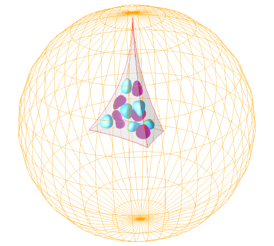
Figure 2: The Picard cell is shown in the unit ball, where the latter is indicated by the yellow net. In addition, the eigenfunction belonging to $k=20.3003\dots$ is shown.

The Picard Universe is now obtained by scaling the hyperbolic metric by $R^{2}$, where $R(t)$ denotes the cosmic scale factor as a function of cosmic time. We consider the standard Robertson-Walker metric within a four-component model consisting of radiation, baryonic matter, cold dark matter, and dark energy, where for simplicity the dark energy is identified with a cosmological constant. Thus, the shape of the Universe is given for all times by the Picard cell which, however, is monotonically expanding. The volume $V(t)=V_{\hbox{\scriptsize Pic}}R^{3}(t)$ and the total energy of the Universe are finite and can be computed. With $\Omega_{\hbox{\scriptsize tot}}=0.95$ and a reduced Hubble constant $h=0.70$, we obtain $V_{0}=0.75\times 10^{32}$ cubic light years for the present day volume of the Universe.

The pattern of the CMB temperature fluctuations $\delta T$ across the sky represents a snapshot of the Universe just $380\,000$ years after the big bang which is, above horizon at recombination, determined (in linear perturbation theory) by the metric perturbation $\Phi$ via the relation $\delta T=F[\Phi]$. (Here $F[\Phi]$ is the linear functional given by the Sachs-Wolfe formula.) Knowing $\Phi$, $\delta T$ can then be computed and expanded into spherical harmonics yielding the CMB angular power spectrum. The gravitational potential $\Phi(t,\vec{x})$ is the central object, which encodes the space-time properties of our Universe at large scales, and can be interpreted as describing the vibrations of space-time within the Universe. The Picard topology defines a kind of three-dimensional drum or cavity whose “sound” is completely determined by the Helmholtz equation for vibrations or, equivalently, the eigenvalue problem of the hyperbolic Laplacian on the Picard topology. It is well-known that the spectrum of eigenvalues (tones) and eigenfunctions of the Laplacian is strongly dependent on the shape, i. e. the topology of the considered manifold (orbifold). And generalizing Marc Kac’s famous question Kac_1966 , we are led to ask: “Can one hear the shape of the Universe?”

If we assume that the Universe is finite, the above question can be positively answered on the basis of Weyl’s law meaning that e. g. the volume of the Universe is uniquely determined if the discrete eigenvalues of the Helmholtz equation for the metric perturbation are known.

The most important property of a finite Universe as compared to an infinite Universe is that the discrete “sound spectrum” has a lowest “tone” which cannot reach the frequency zero due to the existence of a maximal length scale. The sound spectrum we are discussing here and which is constrained by the topology and large-scale structure of the Universe should not be confused with the acoustic oscillations that determine the CMB fluctuations on small scales.

The discrete spectrum of the Picard topology is not known analytically. We have thus calculated the eigenvalues and eigenfunctions (Maass waveforms) numerically. Expressing the eigenvalues $E_{n}$ in terms of the wavenumber $k_{n}$, $E_{n}=k_{n}^{2}+1$, the lowest eigenmode has $k_{1}=6.62211934\dots$. In Figs. 2 and 3 we display the eigenfunctions for $k=20.3003\dots$ and $k=60.0057\dots$. Figures of this type might be called “Chladni figures of the Universe” named after Chladni (1756-1827) who was the first “making sound visible”. Note that all discrete eigenfunctions vanish exponentially if one approaches the cusp. In addition to the discrete spectrum, there is a continuous spectrum which is explicitly given by the Eisenstein series. Here we shall consider the discrete spectrum only. (See Aurich_Lustig_Steiner_Then_2004a for a discussion of the continuous spectrum.)

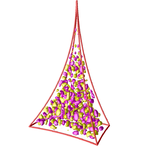
Figure 3: The eigenfunction belonging to $k=60.0057\dots$ is shown in the Picard cell.

In Fig.1 we show as a dashed curve the mean of the CMB correlation function $C(\vartheta)$ of 300 realizations of the primordial anisotropy for a fixed observer using all modes of the Picard Universe for $k\leq 140$. The grey band corresponds to the $1\sigma$ deviation. The contribution of modes with $k>140$ is approximated assuming statistical isotropy and using the density of modes as it is given by Weyl’s law. Here we use $\Omega_{\hbox{\scriptsize mat}}=0.30$, $\Omega_{\hbox{\scriptsize tot}}=0.95$ and $h=0.70$. A scale invariant initial power spectrum $P_{\Phi}(k)\sim 1/k(k^{2}+1)$ is used for the metric perturbation, where the amplitude is determined by the $C_{l}$ spectrum of the WMAP team in the range $l=20\dots 45$. The observer is located at $(0.059,0.029,0.236)$. Fig.1 demonstrates that the Picard topology describes the correlation function much better than the concordance model (dotted curve) since the mean value (dashed curve) is a better match than that of the concordance model. Our theoretical curve displays very small fluctuations at large scales, $\vartheta\gtrsim 60^{\circ}$. The experimentally observed fluctuations by WMAP (solid curve) are for most angles $\vartheta$ within the $1\sigma$ band for the Picard model. In addition, the curve agrees also at smaller scales, $\vartheta\simeq 10^{\circ}$, with the observations much better than the concordance model. For a discussion of the CMB angular power spectrum, see Aurich_Lustig_Steiner_Then_2004a .

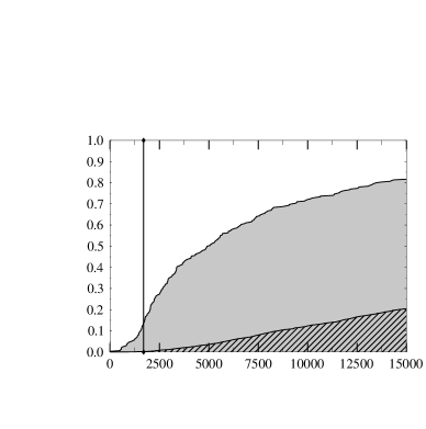
Figure 4: The cumulative distribution of the $S$-statistic for $\alpha=60^{\circ}$ for 300 Picard simulations in comparison to the concordance model. The vertical line shows the value of the $S$-statistic for the WMAP data.

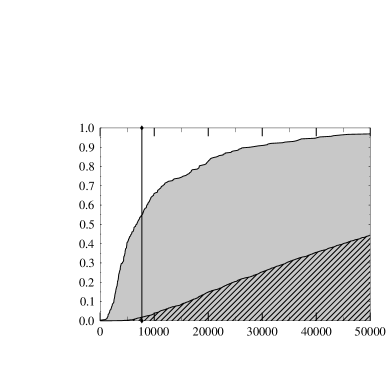
Figure 5: The same as in figure 4, but for $\alpha=20^{\circ}$.

In figure 4 the cumulative distribution of the $S$-statistic is shown for $\alpha=60^{\circ}$ for the Picard model and for the concordance model. From the 3000 Healpix simulations of the concordance model, only 4 models possess values of the $S$-statistic lower than the WMAP value of 1699 corresponding to 0.13% (see also table 1). This contrasts to the Picard topology where 13.3% of the models give values lower than the WMAP value as is seen in figure 4. This difference is also observed for smaller values of $\alpha$, e. g. for $\alpha=20^{\circ}$, shown in figure 5. One obtains 54.3% for the Picard topology and 1.8% for the concordance model. This shows that even for scales down to $20^{\circ}$ the Picard topology gives a better match to the WMAP observation (see also table 1).

It is obvious that our position in the Universe must be “far enough” from the horn of the Picard Universe. Consider the ratio of the volume $V_{\uparrow}$ “above” the observer in the direction of the horn to the total volume $V_{\hbox{\scriptsize Pic}}$, i. e. $V_{\uparrow}/V_{\hbox{\scriptsize Pic}}$. Locating the observer as before, this ratio is $V_{\uparrow}/V_{\hbox{\scriptsize Pic}}\simeq 0.32$, i. e. one third of the total volume lies in the direction of the horn. We have calculated the CMB anisotropy also for an observer very high in the horn having $V_{\uparrow}/V_{\hbox{\scriptsize Pic}}\simeq 0.03$, whose location is thus very unprobable, but even such an extreme position does not betray the horn topology by special temperature fluctuation structures in the CMB maps at or near the position of the horn. It is proven in Petridis_Sarnak_2001 that the eigenfunctions of the Picard topology are quantum unique ergodic, and thus one expects fluctuations of the same statistic in the direction of the horn as in an arbitrary direction. The correlation $C(\vartheta)$ is again suppressed for $\vartheta\gtrsim 20^{\circ}$, and the overall agreement with the WMAP data is better than for the concordance model.

It is claimed that the circles-in-the-sky signature Cornish_Spergel_Starkman_Komatsu_2003 rules out most non-trivial topologies. The linear functional $F[\Phi]$ consists of three main contributions: the naive and integrated Sachs-Wolfe effect, and the Doppler term. Since only the first term reveals the matching circles, it is non-trivial to search for this signature. In Cornish_Spergel_Starkman_Komatsu_2003 such a search is carried out for nearly back-to-back circles, i. e. for circles whose centers have a distance greater than 170^∘ and whose radii are greater than 25^∘ on the sky. The Picard model has no such nearly back-to-back circles and is thus not yet ruled out by this signature. E. g. for the model with $\Omega_{\hbox{\scriptsize mat}}=0.3$ and $\Omega_{\Lambda}=0.65$ for the observer with $V_{\uparrow}/V_{\hbox{\scriptsize Pic}}\simeq 0.32$, there are 40 pairs, where the largest distance of the centers is at 145^∘

$\alpha$	WMAP	concordance	Picard
$60^{\circ}$	1699	40194	9816
$20^{\circ}$	7711	59325	12658

Table 1: The values of the $S$ statistic for the WMAP data and the mean values $\left<S(\alpha)\right>$ for the concordance and the Picard model for $\alpha=60^{\circ}$ and $20^{\circ}$.

The good agreement with the CMB observations does not prove that the Picard topology is the only possible one. In fact, there exist infinitely many hyperbolic three-manifolds/orbifolds with finite volume. It should also be noted that due to the Mostow rigidity theorem Mostow_1973 ; Prasad_1973 , there exist no arbitrary scalings as in the flat case, and the volumes of these three-spaces are topological invariants (for a fixed curvature radius). Here our main point is to show that a hyperbolic Universe with a finite volume is able to describe the observed suppression of power on large scales. Since most hyperbolic three-spaces possess one or more cusps, the Picard topology presents not only a typical, but also one of the simplest possible models for our Universe. Different hyperbolic three-spaces can in principle be discriminated by their different circles-in-the-sky signatures.

For a detailed discussion of the Picard Universe and other models as well as references to earlier work, we refer to Aurich_Lustig_Steiner_Then_2004a .

Financial support by the Deutsche Forschungsgemeinschaft (DFG) under contract No Ste 241/16-1 and the EC Research Training Network HPRN-CT-2000-00103 is gratefully acknowledged.

References

- (1) A. Einstein, Sitzungsber. Preuß. Akad. Wiss. , 142 (1917).
- (2) K. Schwarzschild, Vierteljahrsschrift der Astron. Gesellschaft 35, 337 (1900).
- (3) G. F. Smoot et al., Astrophys. J. Lett. 396, L1 (1992).
- (4) C. L. Bennett et al., Astrophys. J. Supp. 148, 1 (2003), astro-ph/0302207.
- (5) G. Hinshaw et al., Astrophys. J. Lett. 464, L25 (1996).
- (6) K. M. Górski, E. Hivon, and E. B. Wandelt, Analysis issues for large CMB data sets, in Proceedings of the MPA/ESO Cosmology Conference ”Evolution of Large-Scale Structure”, pp. 37–42, 1999, astro-ph/9812350, eds. A.J. Banday, R.S. Sheth and L. Da Costa, PrintPartners Ipskamp, NL (HEALPix web-site: http://www.eso.org/science/healpix).
- (7) D. N. Spergel et al., Astrophys. J. Supp. 148, 175 (2003), astro-ph/0302209.
- (8) G. Efstathiou, Mon. Not. R. Astron. Soc. 348, 885 (2004).
- (9) C. Skordis and J. Silk, astro-ph/0402474 (2004).
- (10) E. Picard, Bull. Soc. Math. France 12, 43 (1884).
- (11) R. Aurich and F. Steiner, Phys. Rev. D67, 123511 (2003), astro-ph/0212471.
- (12) R. Aurich and F. Steiner, International Journal of Modern Physics D 13, 123 (2004), astro-ph/0302264.
- (13) V. G. Gurzadyan et al., International Journal of Modern Physics D 12, 1859 (2003), astro-ph/0210021.
- (14) V. G. Gurzadyan et al., astro-ph/0312305 (2003).
- (15) V. G. Gurzadyan et al., Nuovo Cim. 118B, 1101 (2003), astro-ph/0402399.
- (16) R. Aurich, S. Lustig, F. Steiner, and H. Then, Class. Quant. Grav. 21, 4901 (2004), astro-ph/0403597.
- (17) M. Kac, Amer. Math. Monthly 73, 1 (1966).
- (18) Y. N. Petridis and P. Sarnak, J. Evol. Equ. 1, 277 (2001).
- (19) N. J. Cornish, D. N. Spergel, G. D. Starkman, and E. Komatsu, Phys. Rev. Lett. 92, 201302 (2004), astro-ph/0310233.
- (20) G. D. Mostow, Strong rigidity of locally symmetric spaces Annals of Mathematics Studies No.78 (Princeton University Press, Princeton, 1973).
- (21) G. Prasad, Invent. Math. 21, 255 (1973).