Spectroscopy of Red Giants in the LMC Bar:
Abundances, Kinematics, and the Age-Metallicity Relation

Abstract

We report metallicities and radial velocities derived from spectra at the near-infrared calcium triplet for 373 red giants in a 200 square arcminute area at the optical center of the LMC bar. These are the first spectroscopic abundance measurements of intermediate-age and old field stars in the high surface brightness heart of the LMC. The metallicity distribution is sharply peaked at the median value [Fe/H] = $-$0.40, with a small tail of stars extending down to [Fe/H] $\leq$ $-$2.1; 10% of the red giants are observed to have [Fe/H] $\leq$ $-$0.7. The relative lack of metal-poor stars indicates that the LMC has a “G dwarf” problem, similar to the Milky Way. The abundance distribution can be closely approximated by two Gaussians containing 89% and 11% of the stars, respectively: the first component is centered at [Fe/H] = $-$0.37 with $\sigma$ = 0.15, and the second at [Fe/H] = $-$1.08 with $\sigma$ = 0.46. The dominant population has a similar metallicity distribution to the LMC’s intermediate-age star clusters. The mean heliocentric radial velocity of the sample is 257 km sec^-1, corresponding to the same center of mass velocity as the disk (measured at larger radii). Because of the central location of our field, kinematic constraints are not strong, but there is no evidence that the bar deviates from the general motion of the LMC disk. The velocity dispersion of the whole sample is $\sigma_{v}$ = 24.7 $\pm$0.4 km sec^-1. When cut by metallicity, the most metal-poor 5% of stars ([Fe/H] $<-$1.15) show $\sigma_{v}$ = 40.8 $\pm$1.7 km sec^-1, more than twice the value for the most metal-rich 5%; this suggests that an old, thicker disk, or halo population is present. The age-metallicity relation (AMR) is almost flat during the period from 5–10 Gyr ago, with an apparent scatter of $\pm$0.15 dex about the mean metallicity for a given age. Comparing to chemical evolution models from the literature, we find that a burst of star formation 3 Gyr ago does not reproduce the observed AMR more closely than a steadily declining star-formation rate. The AMR suggests that the epoch of enhanced star formation, if any, must have commenced earlier, $\approx$6 Gyr ago– the exact time is model-dependent. We compare the properties of the LMC and the Galaxy, and discuss our results in the context of models that attempt to use tidal interactions with the Milky Way and Small Magellanic Cloud to explain the star and cluster formation histories of the LMC.

1 Introduction

The Large Magellanic Cloud (LMC) is the nearest actively star-forming galaxy to us, and an invaluable laboratory for the study of stellar and galactic evolution. With a total mass of $\sim$10¹⁰ M_☉ (Westerlund, 1997), the LMC lies just at the borderline between dwarf and giant galaxies, in a regime where the scaling relations of basic galaxy properties (metallicity, mean stellar age, internal structure) with mass undergo a fundamental qualitative change (Kauffmann et al., 2003). Additionally, the LMC is deeply affected by the tidal forces stemming from its interactions with the Small Magellanic Cloud and the Milky Way. Such interactions have been plausibly connected to major events in the lifetime of galaxies, including the creation of bulges, bars, and/or thick disks; and to starburst activity (e.g. Gardiner, 1999).

To accurately measure the histories of star formation and chemical evolution of the LMC is a major challenge for astrophysicists. While general characteristics of its evolution– such as the relatively greater number of stars aged a few gigayears compared to the Milky Way (Butcher, 1977)– have been known for decades, the details are only now able to be measured. For instance, it was not until the construction of the cleanest possible deep color-magnitude diagrams (CMDs) from the WFPC2 camera aboard the Hubble Space Telescope that it became apparent that the variations in field star formation rate have been largely decoupled from variations in the cluster formation rate (Holtzman et al., 1999). Even these modern analyses are not without their difficulties, chiefly the extreme disparity in angular size between the LMC ($>$10⁶ square arcminutes) and the WFPC2 field of view ($\approx$ 5 square arcminutes).

A major factor limiting the precision of star-formation history (SFH) measurements based on deep CMDs is the age-metallicity degeneracy– the fact that age and metallicity can be played off against one another to recreate closely similar distributions of stars in CMDs (e.g., Worthey, 1999). This is exacerbated by the current lack of knowledge of the LMC’s age-metallicity relation (AMR). Star clusters, the most obvious tracers of such a relation, are famously scarce in the LMC for ages between 3–10 Gyr (Da Costa, 1991; Geisler et al., 1997). This age gap spans over half the age of the Universe; it includes the likely epoch of galactic disk formation around redshift $z$ $\approx$1–1.5, and probably spans four LMC-Milky Way orbital periods (e.g., Gardiner, Sawa & Fujimoto, 1994; Bekki et al., 2004). Bekki et al. (2004) draw a connection between the tidal capture of the Small Magellanic Cloud (SMC) by the LMC and the end of the cluster age gap– this capture event had previously been thought unlikely (e.g., Gardiner et al., 1994, and references therein).

For these reasons we have begun to measure the chemical abundances of the field stars in the LMC: to fill in the cluster age gap, to measure the variation of metallicity with radius across the LMC, and to reliably distinguish the bar, disk, and possible thick disk or halo populations from each other. Because the shape of the metallicity distribution function (MDF) is not known a priori, it is important to measure the largest possible sample. The brightest common stars in the age range from $\approx$1–14 Gyr are red giants; in the LMC, they have magnitudes I $\geq$14.8. Because high-dispersion spectroscopy of faint red giants is extremely expensive in telescope time, we rely on spectra of moderate resolution to derive abundances good to $\pm$0.1–0.2 dex by comparison to star clusters of known metallicity. The near-infrared calcium II triplet ($\lambda\approx$8500 Å) is the most widely used such technique. It has been very successfully applied to LMC star clusters, beginning with a landmark paper by Olszewski et al. (1991) (hereafter OSSH). The results from OSSH have become the standard reference for abundances of LMC clusters, and have been used as the basis for simulations of the LMC’s chemical evolution (e.g., Pagel & Tautvaišienė, 1998) (hereafter PT98). The cluster-based AMR has in turn been taken as a guide to the AMR in derivations of the star formation history based on deep color-magnitude diagrams of the field populations (e.g., Gallagher et al., 1996; Geha et al., 1998; Holtzman et al., 1999; Smecker-Hane et al., 2002). It was not feasible to obtain large samples of field star abundances prior to the advent of efficient multi-object spectrographs, first on 4-meter class telescopes, and more recently at 8-meter class telescopes.

We began to obtain abundances for red giants in two fields of the inner LMC disk using long-slit spectroscopy in (Cole et al.2000, Paper I), and expanded the sample six-fold using the Hydra multiobject spectrograph at the Cerro Tololo Inter-American Observatory 4-meter telescope (Smecker-Hane et al., 2004, Paper II). That study found the mean metallicity of red giants at a radius of roughly one disk scale length to be [Fe/H] = $-$0.45, with fewer than 10% of the RGB stars more metal-poor than [Fe/H] = $-$1. We found evidence for a composite kinematic structure of the LMC disk, indicating either a velocity dispersion increasing with age, or a segregation by metallicity into thin and thick disks. Paper II found the inner disk MDF to differ strongly from the only previous field star study, which had targeted a radially distant location (projected radius $\approx$8$\arcdeg$ Olszewski, 1993), in having a much smaller fraction of metal-poor stars and a sharper peak around the median. We used our abundance data and photometry to constrain the age-metallicity relation of the inner disk, finding a slow increase in mean abundance with time.

In this paper, we present our measurements of the chemical abundances and radial velocities of a large number of red giant stars in the highest surface brightness region of the LMC: its bar. Bar fields could not be targeted using Hydra because the wide (2 arcsecond) diameter of its fibers and the difficulties of sky subtraction using fiber systems. We begin by giving some background on the LMC and on the field studied here; this bar field includes the fields singled out for detailed study with WFPC2 by the WFPC2 team (Geha et al., 1998; Holtzman et al., 1999) and by our guest observer program (GO7382; Smecker-Hane et al., 1999a; , Cole et al.2002; Smecker-Hane et al., 2002). Section 2 describes our observing program at the 8.2 meter Yepun (VLT-UT4) telescope at the European Southern Observatory’s Paranal Observatory, and the derivation of metallicities and radial velocites from our spectra. We also discuss how we combine optical photometry and the new metallicity information to estimate the stellar ages of the target red giants. In section 3 we present the bar field MDF, comparing to the Solar neighborhood, other regions of the LMC, and the LMC star clusters. We explore the connection between kinematics and metallicity and how the line of sight velocity dispersion changes with abundance. Section 3.3 compares the derived AMR to the predictions of chemical evolution models based on both smooth and bursting histories of star formation. Our results are summarized and the implications discussed in Section 4.

1.1 Maps & Terminology

To orient the reader and allow us to place our results in a broader context, we show a schematic diagram of the LMC in Figure 1. The map is an Albers equal-area conic projection (Weisstein, 1999) of equatorial coordinates spanning $\approx$11^∘ $\times$ 12^∘. The major large-scale features of the LMC stellar and gas distributions are shown. The solid ellipses follow the smoothed near-infrared isopleths as fit by van der Marel et al. (2001), with semimajor axes of 1, 1.5, 2, 3, 4, 6, and 8 degrees. Within the 2^∘ isopleth, the red starlight is dominated by the bar; outside this radius, the isopleths are elongated towards the Milky Way (van der Marel et al., 2001), and virtually all the stars have disk-like kinematics (Schommer et al., 1992). The rotational center of this disk (van der Marel et al., 2002) is marked by the black square.

As many authors have remarked, the neutral hydrogen distribution is significantly offset from the center of the starlight; we show the kinematic centroid of the H I (Kim et al., 1998) as a black triangle. Major H I features are plotted with dashed lines, following the maps in Staveley-Smith et al. (2003): the main H I disk, roughly 9 kpc across, the archetypal supergiant shell LMC4 near the northern edge of the disk, and several diffuse, tidal arms that spread out from the southeast and the west side of the disk. As noted by Staveley-Smith et al. (2003), the H I distinctly resembles a barred, late-type spiral for velocities between 260–280 km s^-1, with two arms connected by a bridge of gas. We have plotted this bridge in Figure 1, which serves to show that there is no strict morphological relation between the optically-identified bar and any major structure in the gas distribution.

Additional reference points are given by star symbols marking the locations of the two most active star-forming regions in the LMC: the 30 Doradus complex northeast of the bar, and the N11 region near the northwest edge of the H I disk. The distribution of stars— particularly the most recent generations— and gas is incredibly complex and structured on all scales, but this sketch is sufficient to identify the major morphological features that bear on our results. The Galactic center is toward the south; in this representation, the SMC is to the lower right, the orbit of the Clouds carries them to the northeast (towards the Galactic plane), and the LMC’s rotation is clockwise.

The features detailed above place our metallicity and kinematics results into larger context. We have been concerned with five fields, marked by the appropriate alphanumeric tags in Figure 1. Each field contains between 36 and 373 field red giants for which spectra at the Ca II triplet have been obtained. The inner disk fields have been studied by Cole, Smecker-Hane & Gallagher (Cole et al.2000, “D1”, paper I) and Smecker-Hane et al. (2004, “D1” and “D2”, paper II) using the CTIO 4-meter telescope. Results for the transitional disk field (“TD”), so called because of its location near the edge of the H I disk, and the eastern field (“E”) will be reported in a future paper (Cole et al. 2004, in preparation). The bar (“B”) field is effectively located at the heart of the LMC, 0$\fdg$3 from the center-of-rotation of carbon stars (van der Marel et al., 2002). A small number of stars in the outer (“O”) field were observed by Olszewski (1993); these have remained for more than a decade the only abundance measurements of field giants lying outside the gas-rich disk.

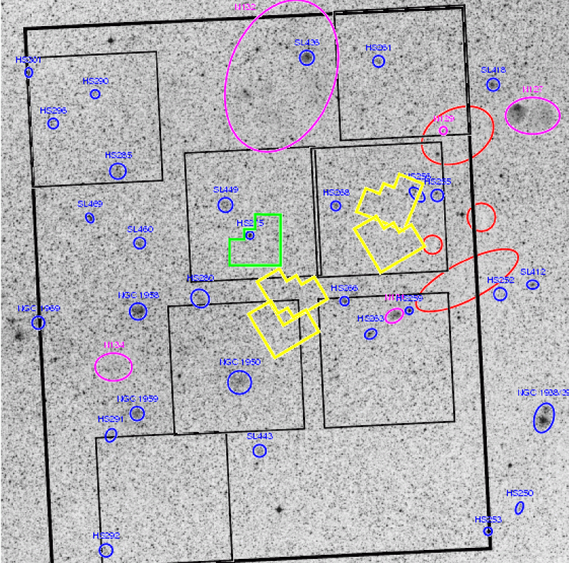
Figure 2: Digitized Sky Survey image of the bar field, centered at ($\alpha_{2000}$, $\delta_{2000}$) = (5^h 24^m, $-$69^∘ 49$\arcmin$) and spanning 30 arcminutes. North is up, East is to the left. The heavy black rectangle shows the region enclosed by $-$70^∘05$\arcmin$ $\leq$ $\delta$ $\leq$ $-$69^∘35$\arcmin$, 5^h22^m $\leq$ $\alpha$ $\leq$ 5^h26^m30^s, within which our seven FORS2 pointings (black squares) are contained. The location of five deep WFPC2 imaging fields useful for measuring the field star-formation history of the bar are oveplotted in yellow (Smecker-Hane et al., 2002) and green (Holtzman et al., 1999). Star clusters and discrete ISM structures have been plotted and labelled following the atlas of Hodge & Wright (1967). Labelled ellipses mark star clusters (blue) and H II regions (magenta). The four red ellipses along the eastern edge of our FORS2 fields mark the positions of dust clouds identified in Hodge (1972).

The remainder of this paper is concerned with the bar field. Figure 2 shows the bar field in more detail, oriented with North at the top and East to the left. The image is in the infrared band of the second Digitized Sky Survey, obtained from the Canadian Astrophysics Data Centre. It is centered at ($\alpha_{2000}$, $\delta_{2000}$) = (5^h24^m, $-$69^∘49′) and spans 30 arcminutes. Within this area are identified 30 star clusters (blue ellipses) and five areas of H$\alpha$ emission (magenta ellipses), labelled following the atlas of Hodge & Wright (1967). Four unlabelled red ellipses mark obscuring dust clouds identified in Hodge (1972). OB associations are notably absent from the field despite its high stellar density. Minor H II regions are present, but easily avoided. The large emission region N132 is a fossil H II region around the oxygen-rich supernova remnant N132D, which probably arose from a Type Ib supernova some 2500 yr ago (Blair et al., 2000). N132D is injecting dense knots of oxygen-rich material into its immediate vicinity (Lasker, 1978), a vivid reminder that the abundances of the red giants measured here are only indirectly related to the present-day gas phase abundances. The region around N132 contains a few blue supergiants in projection (Sanduleak, 1970); this type of stellar population is far more common further west along the bar and northeast towards 30 Doradus. In many places the contribution of intermediate-age and old stars is impossible to isolate cleanly.

Features of the diffuse interstellar medium are omitted for readability, but the field is comparatively simple in structure compared to much of the LMC. The neutral hydrogen in this field is not broken into high- and low-velocity components, as it is in large regions to the northwest and southeast; the H I column density through this field is roughly N_HI = 8$\times$10²⁰ cm^-2 (Luks & Rohlfs, 1992). Two relatively minor molecular clouds, identified based on carbon monoxide line emission at 2.6 mm by Cohen et al. (1988), are found in the southwest corner of the field and much of the east-central portion.

Areas included for study in this paper or related work are also marked. The yellow WFPC2 footprints show the fields in which we have obtained deep images in V and I band in order to create color-magnitude diagrams reaching magnitude $\sim$26 (Smecker-Hane et al., 2002, Cole et al. 2004, in preparation). Similar photometric data were obtained by the WFPC2 team (Geha et al., 1998; Holtzman et al., 1999) in the area marked by the green WFPC2 footprint. The spectroscopic data presented in this paper were obtained within the seven fields shown by the black squares, each of which is 6.8 arcminutes on a side. The heavy black rectangle outlines the region between 5^h22^m $\leq$ $\alpha_{2000}$ $\leq$ 5^h26$\fm$5, $-$70^∘05′ $\leq$ $\delta_{2000}$ $\leq$ $-$69^∘35′; this is a convenient simple border for the irregular region comprised of tiled FORS2 fields.

Overall, the bar field is dense with stars (surface brightness $\Sigma_{\mathrm{V}}$ = 20.7 mag/arcsec²: de Vaucouleurs & Freeman, 1972), but is not a region of strong current star formation or high dust obscuration. Staveley-Smith et al. (2003) estimate the foreground reddening towards the bar field to be E(B$-$V) = 0.06 mag. With the column densities of H I reported in Luks & Rohlfs (1992), and applying the N_HI–E(B$-$V) relation from Koorneef (1982), we make a first estimate of the mean reddening to the giants in our field as E(B$-$V) = 0.08 $\pm$0.02 mag. Some differential reddening is almost certainly present, as will be discussed below. Relatively free of recent activity, the bar field is expected to be an ideal place to study the intermediate-age and old stars of the central regions of the LMC.

While the bar field is as close as practical to the centroid of old (red) stars in the LMC, it is offset from the centroid of bright blue stars, which are more well-aligned with the H I than with the red starlight (e.g. de Vaucouleurs & Freeman, 1972). The flocculent bridge of gas seen in the channel maps of Staveley-Smith et al. (2003) passes just north of our field, and is misaligned with the optical bar. This misalignment is shared with the distributions of very massive main-sequence stars, the brightest red supergiants, and dust-shrouded protostars— the effect is perhaps best seen in the 2MASS starcount maps published by Nikolaev & Weinberg (2000). This population-dependent bar structure is interpreted as being due to evolution of the disk structure over time resulting from a combination of internal and external perturbations (e.g. Dottori et al., 1996).

Owing to time-dependent evolution, it is not particularly meaningful to discuss the “stellar” bar of the LMC, because stars of different ages are distributed differently. The familiar optical bar is perhaps best regarded as a “fossil” bar, while the less distinct bar traced by extreme Population I objects and (possibly) disturbances in the H I velocity field (see, e.g., Kim et al., 1998) can be thought of as a “stelliparous” bar. By comparing the morphologies of different types of stars (e.g. Nikolaev & Weinberg, 2000) and star clusters (e.g. Bica, Claría & Dottori, 1992), we can roughly assign stars more massive than $\approx$6–8 M_☉, and clusters of SWB type (Searle et al., 1980) earlier than III to the stelliparous bar, and older stars to the fossil bar. This puts the age break between the two systems at roughly 70–200 Myr. This is intriguingly close to the epoch of the last major interaction with the Small Magellanic Cloud, an event which could have dramatically redistributed the angular momentum of the LMC disk. Once the bar feature is formed, it can persist for many orbital periods, with the stars born and trapped in the bar comprising a dynamical subsystem of the galaxy (e.g. Sparke & Sellwood, 1987; Shen & Sellwood, 2004).

Throughout the rest of this paper, the term “bar field” will be used to refer to the region shown in Figure 2. Where a broader context is intended, we will use the terms fossil bar and stelliparous bar to distinguish these different morphological systems. It is important to note that the bar is historically defined purely on the basis of optical appearance (Figure 1), and the use of the term does not necessarily imply that a kinematic distinction can be made between populations with different angular momenta and energies at the same location. When population ages are referred to, we will use the terms very young (0–0.2 Gyr), young (0.2–1 Gyr), intermediate-age (1–10 Gyr), and old (10 Gyr). For stellar populations with velocity dispersions of 10–20 km s^-1, 0.2 Gyr is enough time to diffuse throughout the roughly 2.5 kpc length of the fossil bar; since our results primarily concern intermediate-age and old stars, they can be taken as representative of the older populations of the fossil bar.

2 Ca II Spectroscopy

The near-infrared Ca II triplet (CaT) coming from the (3^PD–4^PD) transition is an extremely useful set of lines for the measurement of radial velocities and metallicities in K giants (Armandroff & Da Costa, 1991). The triplet line strength in old, metal-poor red giants can be empirically calibrated for metallicity by removing the influence of surface gravity via a simple linear equation in V magnitude (Rutledge, Hesser & Stetson, Rutledge et al.1997b). This empirical calibration has recently been shown to be applicable to stars nearly as metal-rich as the Sun and as young as 2.5 Gyr (Cole et al., 2004, paper III). The empirical calibration of the CaT to V and [Fe/H] for red giants is supported by theoretical arguments (Jørgensen, Carlsson & Johnson, 1992) as well as by examination of large spectral libraries (Cenarro et al., 2002). The three triplet lines, at $\lambda\lambda$ = 8498, 8542, 8662 Å, are among the strongest spectral features in K giants, and fall neatly between regions of strong telluric H₂O absorption. This has made it an extremely popular method for the measurement of abundances in interemediate-age and old stars in dwarf galaxies throughout the Local Group; the pace of this work has greatly accelerated with the advent of multiobject spectrographs and 8–10 meter class telescopes.

2.1 Target Selection

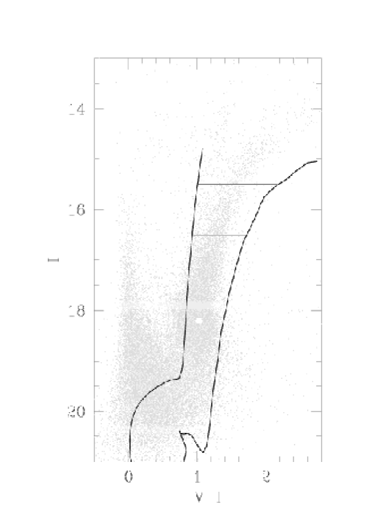
Figure 3: Color-magnitude diagram of the bar field (Smecker-Hane et al., 2004), showing the RGB region between 15.5 $\leq$ I $\leq$ 16.5 from which our targets were selected. Padua isochrones for an age of 2.5 Gyr bound the target region in color; the bluer track has Z = 0.0001, and the redder has Z = 0.019. The white dot marks the centroid of the red clump, which will be used in the metallicity calculation.

We picked our targets to be far enough down the giant branch that we could avoid M stars while still fully sampling the color range of the red giant branch (RGB). Our color-magnitude diagram of the region, obtained at CTIO (Smecker-Hane et al., 2004) is shown in Figure 3, with our targets highlighted by heavy points. We picked our stars to have 15.5 $\leq$ I $\leq$ 16.5, and to have V$-$I colors bracketed by two isochrones with log(t) = 9.40 (age = 2.5 Gyr) from Girardi et al. (2000). The selection region is bounded on the blue side by the Z = 0.0001 ([Fe/H] = $-$2.3) isochrone and on the red by the Z = 0.019 ([Fe/H] = 0.0) isochrone. The selected targets effectively span the observed width of the RGB and so the the exact color limits are not critical to the results. Some stars brighter than the I = 15.5 cutoff were observed when a slit would otherwise have gone unassigned.

Astrometry and photometry for the stars in the central block of four FORS2 fields (see Figure 2) were taken from CTIO data published in Smecker-Hane et al. (2004). These core fields were the originally-intended spatial extent of our spectroscopic survey. However, the southeast quadrant of the core, around NGC 1950, was unexpectedly crowded with very bright stars and appeared to have a large young population (possibly in an unbound corona of cluster stars). Thus we added three additional flanking fields around the region with CTIO photometry. For these flanking fields, we selected targets based on data from the OGLE-II survey (Udalski et al., 2000). Comparison of stars with measurements from both sources found

$$I_{CTIO}=I_{OGLE}-0.007,\;\;\sigma=0.044\;\mathrm{mag},$$

$$(V-I)_{CTIO}=(V-I)_{OGLE}+0.005,\;\;\sigma=0.050\;\mathrm{mag}.$$

For analysis using optical photometry, we use the CTIO photometry, or the transformed OGLE-II photometry.

The position of each target was confirmed using FORS2 preimages obtained in service mode several weeks prior to the observing run, and the slits were assigned using the FORS Instrument Mask Simulator (FIMS) software distributed by ESO.

2.2 Data Acquisition & Reduction

The spectroscopic observations were made in Visitor Mode at the Yepun (VLT-UT4) 8.2-m telescope at ESO’s Paranal Observatory, on the nights of 24–26 December 2002. We used the FORS2 spectrograph in multi-object (MOS) mode, with the 1028z$+$29 grism and OG590$+$32 order blocking filter. In this configuration, the FORS2 field is covered by a mechanical assembly of 19 slit jaws, each 20–22 arcseconds long, that can be arbitrarily positioned along the horizontal (East-West) axis of the field. We chose to use a constant slit-width of 1 arcsecond for ease of calibration. The spectral images were recorded on two 2k$\times$2k MIT/LL CCDs, which have a read noise of 2.7 electrons and an inverse gain of 0.8 $e^{-}$ ADU^-1. The physical pixels were binned 2$\times$2, yielding a plate scale of 0.25 arcsec pixel^-1. The resulting spectra cover 1700 Å, with a central wavelength near 8500 Å and dispersion 0.85 Å pixel^-1 (resolution 2–3 Å). The FORS2 field is 6.8 arcmin across, but is limited to 4.8 arcmin usable width in the dispersion direction in order to keep important spectral features from falling off the ends of the CCD.

The log of observations is given in Table 1, which gives the field names and centers, time of observation, the seeing measured by the differential image motion monitor (DIMM), and the number of RGB targets recovered from each setup. The table includes the same information for the 12 Galactic star clusters that were used as metallicity calibrators (q.v.). Each LMC setup is identified by a number corresponding to its position, and a unique suffix of one or more letters that refers to the slit configuration files produced by FIMS. Each configuration was observed twice, with offsets of 3 arcsec between exposures, to ameliorate the effects of cosmic rays, bad pixels, and sky fringing. The total exposure time in each setup was 2$\times$600 sec, yielding typical signal-to-noise values of S/N $>$30 per pixel. The seeing varied between 0$\farcs$5 $\leq$ FWHM $\leq$ 1$\farcs$4 during the run, with a median value around 0.8 arcsec.

Calibration exposures were taken in daytime, under the FORS2 Instrument Team’s standard calibration plan. These comprised lamp flat-fields with two different illumination configurations and He-Ne-Ar lamp exposures for each slit configuration. Two lamp settings are required for the flat-fields because of parasitic light in the internal FORS2 calibration assembly (T. Szeifert 2003, private communication). Owing to the large number of setups in our program, twilight flats were impractical. All basic data reduction steps were performed under IRAF. We fitted and subtracted the scaled overscan region, trimmed the image, and divided by the appropriately combined lamp flats within the ccdred package.

Spectroscopic extractions were performed with hydra, an IRAF package for handling multislit spectra. Our targets were bright enough that the object trace could be extracted directly from the science exposures. Across the $y$-axis of the CCD, the curvature of the trace along the $x$-direction varied significantly, but could in all cases be fit with a low-order polynomial. Because of the high spectral density and signal-to-noise of night-sky emission lines— primarily OH (Osterbrock & Martel, 1992) and O₂ (Osterbrock et al., 1996)— we used these lines to dispersion correct each spectrum directly instead of using the arc lamps. Typically, the 30 or so strongest emission lines were used in the wavelength solutions, giving a typical root-mean-square (rms) scatter of 0.04–0.08 Å. Because of the scatter in target positions across the dispersion direction of the field, individual spectra can reach wavelengths as blue as 7200 Å, or as red as 10,100 Å; most were centered close to 8500 Å, covering the approximate range 7600 $\leq$ $\lambda$ $\leq$ 9400 Å.

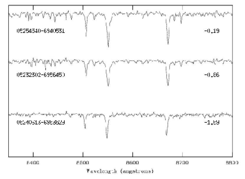
Figure 4: Sample spectra of LMC red giants showing the typical data quality for stars in the fainter half of our sample. All three stars have V $\approx$ 17.5; they are labelled by their 2MASS identifications and metallicities, showing the change in CaT line strength with [Fe/H].

Extraction to one-dimensional spectra was performed within the apall tasks. Sky subtraction was achieved using one-dimensional fits to the background perpendicular to the dispersion direction. Because the targets are bright compared to the sky, and the slits are long compared to the seeing disk, this presented few difficulties. An exception was when the stars fell near the ends of the slitlets; in these cases the sky region was chosen interactively and adjusted to produce the cleanest extracted object spectrum in the region around the CaT. Some stars very close to the top or bottom of the CCD frames showed high sky residuals and were excluded from subsequent analysis. The dispersion-corrected spectra were combined using scombine to minimize the effects of bad pixels and cosmic rays. Each spectrum was continuum normalized by fitting a polynomial to the spectrum, excluding the CaT and regions of strong water vapor absorption. Sample spectra are shown in Figure 4.

Each extracted RGB star and its FORS2 field identifier are listed in Table 2, with the VI magnitudes from the sources listed above. The stars are identified by their number in the 2MASS point source catalogue (Cutri et al., 2003), except where an unambiguous identification was not possible; in these cases the number from the OGLE-II catalogue (Udalski et al., 2000) is used. If a target lies in or around a feature of interest in Figure 2 or has unusual spectral characteristics, this is noted as well. The full table is available in the electronic version of the Journal.

2.3 Radial Velocities

We are interested in stellar radial velocities in order to reject possible foreground Milky Way stars, and to search for correlations between the moments of the velocity distribution and metallicity that could help distinguish between different stellar populations. We performed Fourier cross-correlation (Tonry & Davis, 1979) between our target spectra and the spectra of template stars of known radial velocity. 24 red giants in Galactic star clusters were used as templates; these were a subset of the stars used in our metallicity calibration (Paper III), ensuring a good spectral match between templates and program stars. We used the IRAF fxcor task to perform the cross-correlation, and the radial velocities were found from the average of velocity offsets from each template, weighted by the random error and the height of the correlation peaks. The observed velocities were then corrected to the heliocentric reference frame for subsequent analysis.

Because the stellar image was smaller than the slit width in most cases, there were in many cases slight misalignments between the slit centers and the stellar centroids. This effect propagates into a potentially large systematic error in the observed radial velocity (e.g. Irwin & Tolstoy, 2002). We can correct for this velocity offset if we know the magnitude of the offset in pixels between the centroid of the stellar image and the centerline of the slit on the CCD. Images taken through the slit mask, without the grism, prior to each exposure were used to determine this offset. Each through-slit exposure images a patch of sky $\approx$21 arcsec long by 1 arcsec wide onto the CCD for each target. The stellar centroid is determined by a simple profile fit to the through-slit image, while the position of the slit itself is measured from 1-dimensional fits to the profile of the sky, excluding the stellar flux. The typical offset was less than 0.3 pixels, compared to the slit width of 4 pixels. When a nonzero offset in the dispersion direction was found, we applied corrections to the measured radial velocities based on the dispersion solution measured from the night-sky emission lines. With our spectral resolution of $\approx$29.5 km s^-1 pixel^-1, the resulting velocity corrections ranged from $|\Delta v|$ = 0 to 32 km s^-1, with a mean correction of $-$0.05 km s^-1, and a mean absolute correction of 8.5 km s^-1. We estimate that our centroiding accuracy is roughly a quarter of a pixel, or $\approx$7 km s^-1, and we therefore add this in quadrature to the error in the cross-correlation for our final error estimates. The heliocentric velocities and their associated errors are given in Table 2.

The mean radial velocity of our sample is V_☉ = 257 km s^-1, with a root-mean-square dispersion of 25 km s^-1 about the mean. We found no stars with velocities characteristic of the Milky Way disk (V_☉ $\lesssim$ 100 km s ^-1), and the observed velocity range of 174 km s^-1 $\leq$ V_☉ $\leq$ 336 km s^-1 is entirely consistent with the known range of LMC radial velocities (e.g. Zhao et al., 2003). Some Galactic halo giants have similar velocities, but since they are far fewer in number than disk stars, the contamination rate is negligible. The histogram of heliocentric radial velocities is shown in Figure 5. For comparison to the expected distribution, a thin disk model for the velocity is overplotted: the mean is derived from the equations in van der Marel et al. (2002) to be 260 km s^-1, and the dispersion of 24 km s^-1 is taken from Zhao et al. (2003).

2.4 Equivalent Widths and Abundances

We used the program ew, described in Paper III, to measure the equivalent widths of the CaT lines by fitting each of the three lines by the sum of a Gaussian plus a Lorentzian, constrained to have a common line center. This was deemed necessary to account for the very strong damping wings of the lines. The profile fits were integrated over the line bandpasses (Armandroff & Zinn, 1988) to yield the pseudo-equivalent widths. Error estimates were obtained by measuring the root-mean-square scatter of the data about the profile fits. The summed equivalent widths of the three lines ranged from 3.5 Å $\leq$ $\Sigma$W $\leq$ 10 Å, with typical errors of $\approx$2%. Table 2 gives these values for each target.

Because the relation between CaT equivalent width and metallicity is empirically defined, and because there have been hints that the calibration becomes nonlinear at the high-metallicity end (e.g. Carretta et al., 2001), we observed red giants in 12 Galactic star clusters to define the relation. The clusters span the metallicity range $-$2.0 $\leq$ [Fe/H] $\leq$ $-$0.1, and the age range 2.5 Gyr $\leq$ age $\leq$ $\sim$12 Gyr (see Paper III for details). While many of the bar red giants are probably younger than 2.5 Gyr (q.v.), extrapolation of the calibration to ages $\lesssim$1 Gyr does not seem unreasonable (Cenarro et al., 2002). The calibration relies on the empirical fact that red giants of a single metallicity follow a linear relation between $\Sigma$W and their V magnitude above the horizontal branch, (V$-$V_HB):

$$W^{\prime}([Fe/H])\equiv\Sigma W+0.73(V-V_{HB}),\\$$ (1)

which then leads to the following relation between the reduced equivalent width, W^′, and [Fe/H]:

$$[Fe/H]=(-2.966\pm 0.032)+(0.362\pm 0.014)W^{\prime},\\$$ (2)

with rms scatter $\sigma$ = 0.07 dex. The distribution of target stars in the (V$-$V_HB), $\Sigma$W plane is shown in Figure 6, with isometallicity lines shown for reference. When comparing to abundances of Galactic star clusters, it is important to remember that this calibration is derived with respect to the abundance scale derived by Carretta & Gratton (1997, CG97) for globular clusters, and the compilation of Friel et al. (2002) for open clusters. The globular cluster and open cluster abundance scales are thought to be consistent; work is in progress to obtain a homogeneous set of calcium abundances from high-dispersion spectroscopy for a large sample of clusters so that in the future measurements can be calibrated to a single system (Bosler, 2004).

To derive [Fe/H], we adopt the horizontal branch magnitude V_HB = 19.22, based on our WFPC2 and CTIO photometry (Paper II) Morphologically, this feature is really a red clump and not a horizontal branch in the strict sense (see Figure 3); as shown in Paper III, this does not affect our metallicity determinations. The red clump has a V magnitude dispersion of $\pm$0.12 mag, which we propagate through into our metallicity error estimates. The total random 1$\sigma$ error on each metallicity measurement is 0.1–0.2 dex, with an average value of $\pm$0.14. The derived metallicities and their estimated 1$\sigma$ errors are given in Table 3. The mean of the sample is [Fe/H] = $-$0.45, with a dispersion of $\pm$0.31 dex. However, because of the long tail of metal-poor stars, the median is a better statistical estimator of the of the typical metallicity, which is [Fe/H] = $-$0.40. The interquartile range is $-$0.51 to $-$0.28, and the 10th and 90th percentiles of the distribution are, respectively, $-$0.70 and $-$0.20. The distribution is plotted in Figure 7.

2.5 Derivation of Stellar Ages

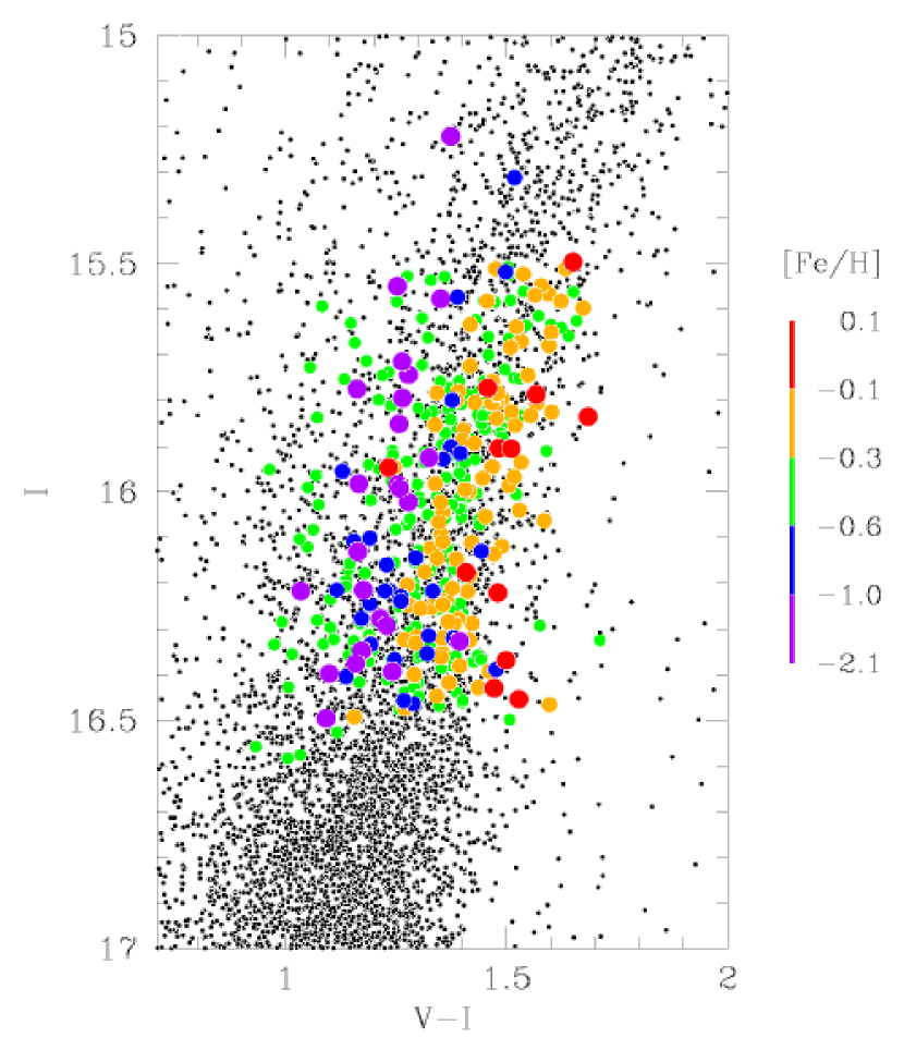
Figure 8: CMD of the bar field RGB; the stars with spectroscopic measurements are color-coded according to their metallicity. For the extreme metal-poor and metal-rich stars the RGB color correlates with metallicity, but stars near the peak of the MDF are scattered across the entire width of the RGB.

An expanded view of the RGB region of the CMD is shown in Figure 8. Spectroscopically observed stars are color-coded by metallicity, with the ranges chosen for clarity of display. It is easily seen that the most metal-poor and metal-rich stars roughly divide themselves in color but stars near the peak of the metallicity distribution, between $-$0.6 $\leq$ [Fe/H] $\leq$ $-$0.3, span the full color width of the RGB. There is even some overlap between stars with [Fe/H] $\approx$ $-$0.2 and $\approx$ $-$0.8. This is a vivid demonstration that where a large age range is present in a stellar population, the mean color of the RGB is an innacurate measure of the metallicity. Some of our faintest, reddest stars are far more metal-poor than would be expected, and could be differentially reddened.

There are two additional points to take from Figure 8: first, that although we searched well to the blue of the bulk of the RGB based on the expectation that metal-poor red giants should be bluer than their metal-rich counterparts, most of the bluest RGB stars are in fact relatively metal-rich; and second, the broad color range of stars at the peak of the MDF is indicative of an extremely large range of stellar ages accompanied by little chemical enrichment over time. This encourages us to quantify the age distribution and age-metallicity relation.

We adopt the procedure described in Paper II to derive isochrone ages for each of our target stars. We use a program developed by one of us (AAC) to place isochrones of arbitrary metallicity in the color-magnitude diagram, and linearly interpolate in the logarithm of the age to find the ([Fe/H], log(t)) pair that reproduces the stellar metallicity and location in the CMD. This is not a precise technique, because the effective temperature of a red giant is principally controlled by its convective envelope opacity, which is largely a function of the abundance of heavy elements in the star (e.g., Hoyle & Schwarzschild, 1955). However, the common perception that the temperature of a red giant is largely independent of its mass is inaccurate.

Hayashi, Hōshi & Sugimoto (Hayashi et al.1962) demonstrated that because red giants are almost entirely convective in their interior they share a common envelope structure. Using analytic homology relations, they showed that when radiation pressure is unimportant, red giants must evolve approximately along tracks described by a relation of the form

$$M^{\frac{1}{2}}\,R^{\frac{3}{2}}=\mathrm{constant}.\\$$ (3)

Using

$$R^{2}=(\frac{L}{4\pi\sigma T_{eff}^{4}})\\$$ (4)

we derive that, insofar as the conditions in the helium core have only a small effect on the outer envelope of the red giant,

$$M^{\frac{1}{2}}\,L^{\frac{3}{4}}\,T_{eff}^{-3}=\mathrm{constant}.\\$$ (5)

Thus from basic physical considerations, we expect that for constant luminosity T_eff $\propto$ M${}^{\frac{1}{6}}$; this is similar to the dependence discovered in numerical models by Sweigart & Gross (1978) and recovered in modern isochrone sets (e.g., Girardi et al., 2000). The magnitude of dT_eff/dM varies with the mass and luminosity of the giant, but is of order 300–500 K/M_☉. In the context of Figure 8, this means that two stars of the same abundance and magnitude will have the same color if they have the same mass (and hence, age). If one star is more massive (younger) than another, it will be bluer. This color difference is translated into an age difference using the published isochrones.

Given representative values of d(V$-$I)/dT_eff (e.g., Bessell, Castelli & Plez, Bessell et al.1998) and the (strongly decreasing) function dM/dt, we find that for perfectly known metallicity and distance, V$-$I photometry good to 2% could be sufficient to provide an age with $\sim$10% accuracy. In practice, random errors in the metallicity measurement dominate the uncertainty, and our typical age errors are of order 60–100% (0.2–0.3 in the log). It is important not to assign undue weight to the age estimate of an individual star, but to use large samples of stars to beat down the random error and thereby glean some information about the mean age-metallicity relation. We tested our technique on a small sample of star clusters in Paper II, and found reasonable agreement with main-sequence turnoff ages, albeit with large scatter. Studies of dwarf spheroidal galaxies (e.g. Tolstoy et al., 2001; Bosler et al., 2004) are generally supportive of the idea that some age information can be gleaned from a combination of accurate RGB metallicities and colors. In the most detailed published study of four dwarf spheroidals (Tolstoy et al., 2003), the derived age distributions showed broad agreement with the star-formation histories derived from main-sequence turnoff photometry. However, a significant decrease in sensitivity was noted for abundances much below [Fe/H] $\lesssim$ $-$1. An in-progress study of fifty-eight red giants in the Carina dwarf spheroidal by one of us (TSH) will make an extremely interesting test case; first indications are that the most metal-rich stars ([Fe/H] $>$ $-$1.5) are on average a factor of four younger than the stars with [Fe/H] $<$ $-$2. However, finite errors on the observed metallicities (see Smecker-Hane et al., 1999b) make it unlikely that RGB-derived ages will ever clearly resolve the discrete epochs of star-formation derived from main-sequence turnoff photometry as in Hurley-Keller, Mateo & Nemec (1998).

A potentially major contributor to the error budget is the uncertainty in relative abundances of the various elements heavier than helium. Because the LMC has experienced a different chemical evolution history than the Milky Way, the scaled-Solar abudance ratios cannot be assumed to apply. Evidence for changing values of [O/Fe] with [Fe/H] in LMC field red giants has been presented by Smith et al. (2002) and the amount of data is increasing rapidly (Hill et al., in preparation). Hill et al. (2000) and Johnson et al. (2004) have also measured the changing abundance of $\alpha$-process elements relative to iron in several massive LMC star clusters, finding important differences between the LMC globulars and the standard Milky Way Population II abundance mixture. Because the $\alpha$ elements are major electron donors in red giant envelopes, [$\alpha$/Fe] ratios play a major role in determining the stellar T_eff (e.g., Salaris, Chieffi & Straniero, Salaris et al.1993). Therefore it is vital in attempting to age date a red giant with isochrones that the correct relative abundance blend is used. For practical purposes, we represent all deviations from the scaled-Solar abundance mixture using the parameter [$\alpha$/Fe], and adopt the approximate relation between the overall abundance of electron donors, [M/H], and [$\alpha$/Fe] given by (Salaris et al.1993):

$$\mathrm{[M/H]}\approx\mathrm{[Fe/H]}+\log(0.638\;10^{[\alpha/Fe]}\;+0.362).\\$$

Because of the limited amount of data available, we make the simplifying assumption that [$\alpha$/Fe] = [O/Fe]. Combining the data from Smith et al. (2002) and the preliminary results from Hill et al. (in preparation), we approximate the trend of [O/Fe] with [Fe/H] by a bilinear relation:

$$[\alpha/\mathrm{Fe}]=\left\{\begin{array}[]{r@{\quad:\quad}l}0.05-0.10\,[\mathrm{Fe/H}]&[\mathrm{Fe/H}]\leq-1\\ -0.413-0.563\,[\mathrm{Fe/H}]&[\mathrm{Fe/H}]>-1\end{array}\right.$$

There seems to be scatter of 0.1–0.2 dex about the mean [O/Fe] at given [Fe/H], but this is not definitely larger than the measurement uncertainty. The values of [$\alpha$/Fe] adopted for purposes of the age calculation are included in Table 3.

We adopt the LMC “standard” distance of 50.1 kpc, based on the distance modulus adopted by the HST Key Project to determine H₀ (Freedman et al., 2001); adopting the LMC disk structure from van der Marel et al. (2001), the bar field is 0.1 kpc more distant than the LMC center of mass, giving a distance modulus (m$-$M)₀(bar) = 18.50. This value is slightly higher than (but in good agreement with) more recent distance determinations based on eclipsing variables (Fitzpatrick et al., 2003) and RR Lyrae stars (Alcock et al., 2004). Because of this good agreement, we adopt an errorbar of $\pm$0.06 mag in the distance modulus. We adopt a reddening value E(B$-$V) = 0.06 $\pm$0.03 based on the discussion in Staveley-Smith et al. (2003) (also see Cole, Smecker-Hane & Mandushev, Cole et al.2002; Skillman & Gallart, 2002).

The Padua isochrones include stars as old as log(Age/Gyr) = 10.25 (Age = 17.8 Gyr). These were calculated in order to match the horizontal branch morphology of the oldest globular clusters, given what was known about their distances and the parameterization for stellar mass loss that went into the models. There is now very strong evidence from the first year of data from the WMAP satellite that the Universe is 13.7 Gyr old (Spergel et al., 2003). In the meantime, both revisions in the cluster distance scale (e.g. Reid, 1999) and updated stellar interior calculations (e.g. VandenBerg et al., 2002) have produced a strong expectation that the oldest globular clusters are no more than $\approx$13.5 Gyr old. While these argue for an age bias in the Padua isochrones at the old end of the scale, there is much support for their accuracy at intermediate ages. Studies of clusters (Bonatto, Bica & Girardi, 2004; Salaris, Weiss & Percival, 2004) and the field (Binney, Dehnen & Bertelli, 2000) have derived ages for the oldest open clusters and the oldest stars in the Solar neighborhood in the range of 9–11 Gyr. These are in excellent agreement with independent measurements of the age of the Milky Way disk: $\approx$9 Gyr from thorium cosmochronometry (Morell, Källender, & Butcher, 1992) and from the faint end of the white dwarf luminosity function (Leggett, Ruiz & Bergeron, 1998; Hansen & Liebert, 2003). To bring the results for our oldest stars into agreement with the known age of the Universe, while at the same time preserving the success of isochrone measurements of the age of the Galactic disk, we adopt the expedient of simply rescaling any ages older than 10 Gyr. In the absence of detailed information, we use a linear function

$$\mathrm{Age}=10+0.41\;(\mathrm{Age_{raw}}\;-10)\quad\mathrm{(Gyr)}.\\$$

The average age shift for the ten stars affected is $-$1.3 Gyr, well within the uncertainty in absolute age-dating of any old stellar population, and negligible compared to the measurement error in our method. Because we adopt broad age bins in our analysis of the age-metallicity relation, the exact prescription for enforcing consistency between isochrone ages and the age of the Universe has very little effect on our results.

There is ambiguity in the derived ages, because the evolutionary status of a star of given L, T_eff, [Fe/H], and [$\alpha$/Fe] is not known a priori. We have assumed that all stars are first-ascent red giants, except where the isochrones invalidate the assumption; in these cases the age has been derived assuming the star in on the asymptotic giant branch. If an assumed RGB star is in fact on the AGB, our derived age will be roughly 30% too young. The derived age estimates and random errors, expressed in logarithmic scale, are given in Table 3. There is a concentration of stars at 13.7 Gyr caused by eleven stars that were too red for the oldest isochrone, the ages of which were set equal to the age of the Universe (log A = 10.13). For our choice of isochrone set, reddening, and [$\alpha$/Fe] ratios, the median age of RGB stars in the bar field is 2 Gyr. The interquartile age range is 1.4–3.4 Gyr, and 90% of the RGB stars in this field are younger than 6 Gyr.

3 Interpretation & Analysis

3.1 The Metallicity Distribution Function

The bar field MDF (Fig. 7) is a basic datum that should provide strong new constraints on the inferred history of the LMC bar based on color-magnitude diagram or spectral synthesis studies. The mean and dispersion of [Fe/H] = $-$0.45 (systematic error $\approx$ $\pm$0.1 dex), $\sigma$ = 0.31 are not very meaningful statistical descriptors of the data, owing to the strong asymmetry of the distribution. A maximum-likelihood analysis was used to fit two Gaussian distributions to the unbinned data; the resulting curve is plotted over the histogram in Figure 7. The curve is split into a narrow, metal-rich distribution containing 89% of the stars, with the remainder in a broad, metal-poor distribution. The major population is described by mean $\mu_{1}$ = $-$0.37 and $\sigma_{1}$ = 0.15, and the minor component by $\mu_{2}$ = $-$1.08 and $\sigma_{2}$ = 0.46. $\sigma_{1}$ is barely larger than our measurement error, suggesting either that we have been too conservative in our error estimates or that the intrinsic astrophysical spread in metallicity is less than $\pm$0.05 dex for this component.

The fraction of metal-poor stars is much smaller than in the abundance distribution of long-lived main-sequence stars in the Solar neighborhood (e.g., Kotoneva et al., 2002). However, there are strong systematic effects due to the RGB lifetime that make this comparison inappropriate. The bar field red giant MDF is better compared to the Solar neighborhood data for G and K type giants brighter than V $\approx$ 5.5 obtained by McWilliam (1990). The two distributions are shown in Figure 9. The Solar neighborhood MDF shows a similar narrow peak at high metallicity, but is even more deficient in stars with [Fe/H] $\leq$ $-$0.8. The peak of the McWilliam (metal-rich bar) sample is at [Fe/H] = $-$0.17 ($-$0.37) and the dispersion is $\sigma$ = 0.16 (0.15) dex.

We can make a direct comparison to the abundance distribution of the LMC cluster system taken from the OSSH paper. OSSH give abundance measurements for 70 clusters located across the body of the LMC, taken from similar spectra to those obtained here. Their equivalent widths are calibrated to globular and open clusters on a metallicity scale different from the one we use (Paper III). By making a least-squares fit to the calibrating cluster abundances, we adopt an estimated cluster abundance scale

$$\mathrm{[Fe/H]_{clus}}\approx-0.212+0.498\,\mathrm{[Fe/H]_{OSSH}}-0.128\,\mathrm{[Fe/H]^{2}_{OSSH}}.\\$$ (6)

This recalibration explicitly includes the open clusters M67 and Melotte 66, and so supersedes that presented in Paper II, which was taken from CG97, with ad hoc modifications above [Fe/H] = $-$0.5. Note that some recent measurements of a subset of LMC clusters at high resolution and signal-to-noise support a recalibration of the OSSH measurements, while others support the original OSSH results (e.g., Hill et al., 2000; Johnson et al., 2004). These recent studies primarily concern clusters with [Fe/H] $\lesssim$ $-$0.9.

The histogram of recalibrated cluster abundances is plotted with our bar field data in Figure 10. The cluster MDF is distinctly bimodal, which presents a visual contrast with the long metal-poor tail of the bar field MDF. The main peak of the cluster MDF, corresponding to the $\approx$1–3 Gyr old clusters, matches up well with the peak of the bar field MDF, but may be more asymmetric towards lower metallicities. Just such a relationship would be predicted by a model of star formation in which cluster formation events are shorter and more intense than field star formation episodes (e.g, Bekki et al., 2004). However, we caution against overinterpreting the comparison in Figure 10, because of the uncertainties introduced by the different metallicity scales.

Two additional factors are the accelerated pace of stellar evolution at low metallicity, and the decrease with increasing age of the mass range sampled by our RGB selection region. This effect (discussed in detail in Paper II) effectively biases us against detection of the older and more metal-poor stars in the field. This must be taken into consideration when comparing the cluster and field star MDFs. For example, 5% of the field RGB stars in the bar have metallicities in the range $-$1.5 $\leq$ [Fe/H] $\leq$ $-$0.9; the same fraction of clusters (4 out of 70, or 6 $\pm$3%) fall in this range. Because of the bias against metal-poor field giants, the true relative fraction of astrated mass in this metallicity range is likely to be some 2–3 times higher, erasing any suggestion that the bar field MDF has a bimodality similar to the cluster MDF. This effect should apply even more strongly to the most metal-poor (oldest) field stars, bringing the observed fraction of metal-poor stars with [Fe/H] $<$ $-$1.5 (4%) approximately into line with the observed cluster fraction below $-$1.5, that is, 8 out of 70 (11 $\pm$4%). Because of the strong role of stellar age in determining the number of RGB stars in our selection window per unit stellar mass created, a detailed comparison of the field star and cluster metallicity distributions must await a joint analysis of the color-magnitude diagram and metallicity distribution together.

Independently of metallicity scales and sample biases, the bar field MDF has a different shape (unimodal with tail) than does the cluster sample (bimodal with slight overlap). This confirms the trend found in the inner disk in Paper II, and extends it into the center of the LMC. We find that the bar field is closer in shape to the cluster MDF than the inner disk samples in Paper II. For example, the fraction of field stars falling into the cluster metallicity gap is smaller in the bar field (5%) than in Disk 1 (13%) or Disk 2 (11%), despite the bluer color extent of the sample selection region in the current study. This is probably indicative of the higher fraction of intermediate-age stars in the bar compared to the disk, expected on both observational (Smecker-Hane et al., 2002) and theoretical (Bekki et al., 2004) grounds.

The mean metallicity of our sample of bar field red giants is [Fe/H]_B = $-$0.45, essentially indistinguishable from that of the D2 field, [Fe/H]_D2 = $-$0.46. Both are more than 0.1 dex more metal-rich than the D1 field that has [Fe/H]_D1 = $-$0.59. The offset is many times the formal random error and is highly significant. All three fields have similar dispersions about the mean metallicity, $\sigma_{[Fe/H]}$ = 0.32 $\pm$0.01. The difference between D1 and the other fields may be related to the location of the D2 field at the end of the bar and the D1 field in a region of much lower surface brightness, far outside the bar-distorted isophotes. More data, in widely varying locations, is required before any firm conclusion about the possibility of spatial variation in mean metallicity can be reached. Because of the different selection effects, and the imminent addition of data from other locations in the LMC (the Transitional Disk and Eastern fields, see Figure 1), we defer a detailed comparison of the bar and disk fields to a future paper.

3.2 Stellar Kinematics at the LMC Center

The radial velocity of our sample is entirely consistent with the disk rotation curve derived by van der Marel et al. (2002) from carbon star velocities, mostly at projected angular radii greater than 2$\arcdeg$. Because our field is located almost directly at the rotation center of the disk, the rotation signature is expected to be small. Therefore we cannot rule out the presence of a non-rotating (halo or bulge) or slowly-rotating (thick disk) disk component with these data.

Stars on bar orbits are expected to show large streaming motions along the long axis of the bar (e.g. Sparke & Sellwood, 1987). These could amount to several tens of kilometers per second, which would produce a signature in the radial velocity data as long as the bar does not lie in or nearly in the plane of the sky. Detailed predictions for the kinematic signature of off-center bars in dwarf galaxies are unavailable, but it seems likely that stars on bar orbits could be contributing to the non-Gaussianity in the observed velocity field (Fig. 5). Such non-circular motions could also be contributing to the line of sight velocity dispersion, which is higher than that predicted by the thin disk model of van der Marel et al. (2002).

The velocity dispersion along the line of sight is $\sigma$ = 24.7 $\pm$0.4 km s^-1, in excellent agreement with the general sample of LMC stars measured by Zhao et al. (2003). The dispersion is slightly higher than the value of 20 km s^-1 reported for the global average of LMC carbon stars by van der Marel et al. (2002), and 60% higher than the 16 km s^-1 line of sight velocity dispersion of H I gas reported by Kim et al. (1998). While the measured dispersion suggests a moderately thick structure, it is not high enough to imply that the majority of stars occupy a dynamically hot population such as a bulge or halo. It was suggested by Zaritsky (2004) that such a structure could account for some observations of the morphology and structure of the inner LMC and give the appearance of a bar.

For many years, studies of the intermediate-age and old populations in the LMC have found increased velocity dispersions with age, up to a limit of roughly 30–35 km s^-1 (e.g. Hughes et al., 1991; Schommer et al., 1992). Even the oldest star clusters appeared to form a thick disk rather than a spheroid (Freeman et al., 1983; Schommer et al., 1992). By contrast, Minniti et al. (2003) have found a velocity dispersion of 53 km s^-1 for the RR Lyrae type variables in the area of the bar. These values roughly bracket what might be generally expected for a kinematically hot halo in the potential of the LMC (M $\approx$ 10¹⁰ M_☉).

We can test our sample for similar effects by dividing into several subsamples. Following the procedure in Paper II, we show the line of sight velocity dispersion of samples in various metallicity ranges in Table 4. The plot of radial velocity vs. metallicity is given in Figure 11, showing that while the metal-rich and metal-poor stars share a total velocity range of over 100 km s^-1, the bulk of the stars are far more concentrated towards the mean than the stars more metal-poor than [Fe/H] $\approx$ $-$1. The mean radial velocity barely changes with metallicity. The dispersion starts at 16.7 $\pm$1.6 km s^-1 for the most metal-rich (and presumably youngest) stars, increases dramatically by the next metallicity bin, and then gradually grows with decreasing metallicity until the last bin, when another large jump brings the line of sight dispersion of the stars below [Fe/H] = $-$1.15 to 40.8 $\pm$1.7 km s^-1. Note that this is completely in line with the expected line of sight velocity dispersion for a halo population, but our sample has neither the size nor the spatial extent to measure any deviations from a rotating disk among this minority population.

Zaritsky (2004) proposed that the optically-identifed LMC bar is actually a triaxial bulge. If we take its luminosity to be of order $\sim$10⁸ L_B,☉, then the Faber-Jackson relation would predict a velocity dispersion in the neighborhood of $\approx$70 km s^-1 for a classical bulge. Such structures are not associated with late-type galaxies like the LMC; on the other hand, barred galaxies are strongly connected with the presence of box- or peanut-shaped pseudobulges (e.g., the very thorough review by Kormendy & Kennicutt, 2004). The creation of pseudobulges, which are dynamically colder than classical bulges, is linked to secular dynamical evolution of the disk and bar. A pseudobulge in the LMC would likely have a velocity dispersion of $\approx$30–40 km s^-1, in agreement with what we observe for our most metal-poor subsample of stars. However, pseudobulges are created from the general disk and bar stellar populations, and so there is no expectation that they should be preferentially more metal-poor than their surroundings. Indeed, Peletier & Balcells (1996) have found that the stellar populations of pseudobulges are indistinguishable from those of the disks in which they are embedded. This strongly suggests that the small fraction of stars we observe at high velocity dispersion and low metallicity does not owe its existence to the secular heating of the disk by the bar. Irrespective of nomenclature (“halo”, “bulge”, or “pseudobulge”) the dynamically hot population population in the central LMC is a very minor contributor to the total stellar surface density.

The velocity dispersion we measure is comparable to our D1 and D2 results from Paper II. We do not attempt to break our bar sample into thin and thick disk components, because of the unknown influence of the bar on disk structure and because the distribution in Figure 5 is not particularly well-fit by two Gaussians. The probability is that the stellar populations are characterized by a continuum of velocity dispersions, rising with age due to gravitational scattering. It is interesting to note that the most metal-rich stars are not significantly hotter than the neutral ISM, suggesting either that the stellar disk was not strongly heated by the most recent encounter with the SMC, $\approx$200 Myr ago, or that the continuing gravitational interactions with the Milky Way and SMC have kept the H I from cooling below this level.

3.3 The Age-Metallicity Relation

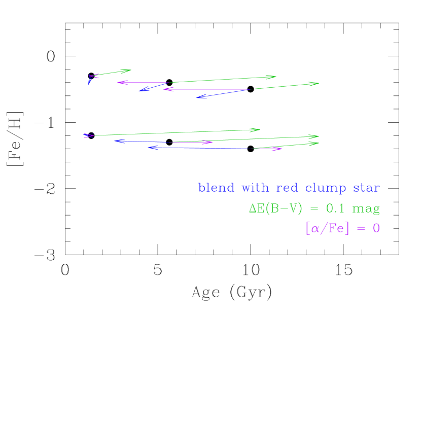
Figure 13: Illustration of the systematic effects of stellar crowding, differential reddening, and variable abundance ratios on the age estimates presented here. Black circles mark the “true” locations of test RGB stars in the age-metallicity plane, and the arrows show how the measured values would appear to change as a result of the listed effects.

The derived age-metallicity plot is shown in Figure 12. Typical errorbars are shown at the bottom of the plot for clarity. At a given age, there is a large scatter in metallicity. Part of this is certainly a real scatter, and part of it stems from systematic effects such as differential reddening or incorrect assumptions about the [$\alpha$/Fe] ratio. These effects are illustrated in Figure 13. In this diagram the locations of six “test” RGB stars with I = 16 have been plotted in the age-metallicity plane. Arrows show how the derived ages would change if the stellar spectra were contaminated with that of a red clump star of [Fe/H] = $-$0.4 (blue arrows), if the star was reddened by an additional 0.1 mag in E(B$-$V) (green arrows), or if the [$\alpha$/Fe] ratio had been assumed to be Solar instead of following the LMC trend (e.g., Smith et al., 2002). Note that the metallicity measurements are robust against these effects, which primarily affect the age estimates.

We find 14 stars with [Fe/H] $<-$1 and age $<$ 10 Gyr. Similar populations are much less common in the data for the D1 and D2 fields (Paper II). This is not an artifact of the different selection criteria adopted: only one of these stars lies blueward of the adopted edge of the selection region in the earlier paper. As we might expect, most of the stars that the D1 and D2 selection regions would have missed are quite young, with an average age below 0.5 Gyr. The presence of these stars at the blue side of the RGB indicates that young stars are much more prevalent in the bar than in the disk at a radius of one scale length. The results of Figure 13 suggest that some fraction of the apparent intermediate-age, metal-poor stars may be unresolved blends of genuinely ancient, metal-poor stars with intermediate-age red clump stars near the peak of the MDF. A higher percentage of blended stars in the bar than in the disk would naturally be expected because of the much higher stellar surface density in the bar field. Some evidence in favor of this interpretation can be taken from the radial velocities and age estimates of the two stars that have [Fe/H] $<-$1 that were flagged during data reduction as having faint companions (Table 2). 2MASS point sources 05225632-6942269 and 05253235-6943137 have ages, respectively, of 1.9 $\pm$0.8 Gyr and 7.6 $\pm$5 Gyr, much younger than average for their metallicities of $-$1.19 and $-$1.61. Depending on the properties of the faint companion objects, their true ages could be much older.

Because of the large random errors (up to a factor of two) and the possibility that systematic effects may ruin some individual estimates, the age information is most usefully interpreted when binned up to increase signal-to-noise and suppress the effects of outliers. We sort the stars into five equal-age bins 2.7 Gyr wide, and show the mean metallicity in each bin in Figure 14. The five faintest, reddest stars, measured perpendicular to the RGB ridgeline (see Fig. 8), have been excluded from the averaging because differential reddening is suspected. The vertical errorbars on each point show the rms scatter about the mean in each bin, and the horizontal bars denote the extent of the bin. The area of each point is proportional to the number of stars in the bin, ranging from 10 in the oldest bin to 255 in the youngest.

Figure 14 shows that the metallicity steadily increases with time: quickly at ancient times, and then by $\lesssim$0.5 dex over the past 10 Gyr. The metallicity scatter appears to decrease with time, from $\pm$0.5 dex in the oldest bin to $\pm$0.2 dex in the youngest. For the oldest bin, the likely culprit is the requisite rapidity of chemical evolution from [Fe/H] $\approx$ $-$3 at the end of the Population III phase to $\approx$ $-$1 within the first 4 Gyr. The fact that the errors in our age estimate are large for the oldest stars probably introduces additional scatter by creating mixing between age bins.

The age-metallicity relation we derive is compared to the results from studies that have focused on specific sub-populations of stars in Table 5. The first two lines recapitulate the two Gaussian fits to the MDF derived in section 3.1. Based on the derived ages, the two metallicity components are split into young and old populations, although there is obviously considerable overlap between them. The remainder of the table shows the mean metallicities and dispersions of various stellar populations, arranged by increasing age. Where we have been able to trace the published abundances back to a scale similar to that used by OSSH, we have applied Equation 6 to bring the values into line with our data. The picture is one of rapid evolution at early times, followed by a very slight increase over the past 10 Gyr.

B dwarfs and Cepheids are taken to be representative of the very young stellar populations; their mean abundance is only very slightly higher than the peak of the metal-rich component of the field giant MDF in the bar. Evidently the chemical evolution of the LMC has been quite modest over the past $\sim$10⁹ years. Very few tracers of chemical evolution at intermediate age have been available to date; the sample of planetary nebulae measured by Dopita et al. (1997) contains very few objects older than the oldest intermediate-age star clusters. The only star cluster with an age of 4–10 Gyr is ESO121-3, with [Fe/H] = $-$0.93 (OSSH; Hill et al., 2000). Although the AMR appears shallow, we find the mean metallicity of stars aged 3–6 Gyr to be [Fe/H] = $-$0.46 $\pm$0.02, compared to $-$0.72 $\pm$0.03 for the stars aged 6–8 Gyr, nearly a factor of two difference.

The low-metallicity component of our MDF is more metal-rich than the average of old star clusters or field RR Lyrae variables, with a higher dispersion. This indicates the continuous nature of field star formation, in that we have probed a much wider range of the LMC’s history than just the oldest populations traced by the globular clusters and RR Lyraes. If we just consider the 14 stars estimated to be older than 10 Gyr and not suspected of differential reddening, the mean [Fe/H] = $-$1.31, with a dispersion of $\pm$0.51. This is consistent with the field RR Lyrae stars of the bar, although the dispersion is larger than the value of $\pm$0.29 dex in the RR Lyrae sample of Gratton et al. (2004).

3.3.1 Comparison to Models

Models for the chemical evolution of the LMC (Pagel & Tautvaišienė, 1998, (PT98)), based on two different assumed star formation histories and with the yields adjusted to fit the ancient globular clusters and the numerous clusters aged 1–3 Gyr, are overplotted on our binned age-metallicity relation. The dashed line shows the chemical evolution derived from assuming that the star-formation rate had a broad peak $\approx$10 Gyr ago and has been very slowly declining since then. The solid line marks instead the chemical history of a model LMC with roughly constant low level of star formation for most of its history, that then experienced a factor of six jump in star formation rate 3 Gyr ago, with a subsequent rapid decline. Both smooth and bursting classes of SFH can reproduce the star cluster age-metallicity relation, owing to the lack of clusters between 3–10 Gyr old.

As found in D1 and D2, the field stars fill in the cluster age gap with a continuous distribution of ages and metallicities. This raises the possibility that we can statistically distinguish between the two cases. It can be seen from Figure 14 that stars aged from $\approx$2–10 Gyr will have the strongest lever on the models, with little to differentiate between them at the oldest and youngest times. For each observed star, we start from the age derived in Table 3 and calculate the probability that it was drawn from the age-metallicity relation appropriate to the bursting or the smooth model, taking the observational error on [Fe/H] into account. The relative likelihoods of the models are then computed by finding the joint probability of observing the entire ensemble of stars under each model. The amount of cosmic scatter assumed in the model AMR will influence the results, so we adopt $\sigma_{\mathrm{AMR}}$ = 0.15 as a realistic estimate.

We find that the observed AMR is better matched by the smooth model from PT98 than their 3-Gyr burst model at the 2$\sigma$ level (95.8% confidence). While the latter is a better match to the stars aged 5–10 Gyr, these stars are greatly outnumbered by younger stars, which have higher abundances than predicted by the burst model. However, many lines of evidence point to a bursting history of star fomation in the LMC. Smecker-Hane et al. (2002) have shown that the epoch of increased star formation rate in our bar field is likely to have occurred earlier than 3 Gyr ago. Figure 14 makes plain that an earlier burst can be tuned to match the stars both older and younger than 5 Gyr, and so can be made to be fit the data better than the smooth model. Based on the shape of the AMR predicted by PT98’s bursting model, a burst would be expected to have occurred prior to $\approx$5 Gyr ago, but not much before $\approx$7 Gyr.

Because of the low precision of our age estimates and the uncertainties in computing chemical evolution models, a maximum likelihood calculation of the time and amplitude of a starburst from these data is unlikely to produce meaningful astrophysical results. We defer such an exercise to a future paper, in which we will simultaneously model the full WFPC2 CMDs down to below the oldest main-sequence turnoff and the red giant MDF derived here.

3.4 Spatial Patterns & Clustering

We attempted to avoid star clusters and associations as much as possible, but three stars projected directly on two clusters (HS 256 and HS 285) crept into the measured sample. An additional thirteen stars (identified in Table 2) in the close vicinity of five star clusters were also measured. Considering the field density and the apparent blue colors of the clusters on our preimages, it is unlikely that the stars in the neighborhoods of the small clusters are bona fide members.

Neither HS 256 nor HS 285 has a published age in the literature. HS 256 partially overlaps with one of our WFPC2 fields, so it may be possible to examine its color-magnitude diagram separately from the field in a future paper. Two stars of our sample, 2MASS 05223416-6944433 and 05223895-6945007, are seen in projection against HS 256. Their radial velocities are both very low compared to the sample mean, 222 and 227 km sec^-1 respectively, which may indicate their joint membership in a population with low velocity dispersion moving towards us at 30 km sec^-1 relative to the mean bar field. However, the two stars have very different metallicities: [Fe/H] = $-$1.05 $\pm$0.12 and $-$0.42 $\pm$0.14. There is no reason to suspect the quality of the abundance measurement in either star, but the widely discrepant values militate against common cluster membership. The single star seen in projection against HS 285 is indistinguishable from the general field in both its radial velocity (261 km sec^-1) and metallicity ($-$0.37).

We examined maps of the area, searching for spatial patterns in the radial velocity, metallicity, and age of the stars. No strong evidence for structure in the populations was observed. However, there did appear to be a slight concentration of the reddest stars into the southwest corner of the field, near the largest of the dark clouds identified by Hodge, and some small, chainlike H II regions (see Figure 1). When comparing the 2MASS J$-$K colors of the stars, we found the reddest stars to be far more evenly dispersed throughout the bar field. Because the J$-$K color is less affected by reddening than is V$-$I, this is consistent with our interpretation that the concentration of stars with high V$-$I is not the effect of high metallicity or old age.

4 Summary & Discussion

The high surface brightness and extreme crowding of the central regions of the Large Magellanic Cloud have challenged observers for decades. In this paper, we present the first spectroscopic study of the abundances, kinematics, and age-metallicity relation for field red giants in the LMC bar. Taking advantage of the superb image quality and efficiency of the FORS2 spectrograph at VLT-UT4 (Yepun), we obtained spectra of 373 red giants in a 200 square arcminute region of the central bar that includes several fields singled out for detailed photometric study with WFPC2 (Holtzman et al., 1999; Smecker-Hane et al., 2002).

We have derived abundances on a metallicity scale consistent with those of CG97 (globular clusters) and Friel et al. (2002, open clusters) (Paper III), with internal accuracy of $\pm$0.14 dex per star. Radial velocities accurate to $\pm$7.5 km s^-1 were measured by Fourier cross-correlation of our spectra with template stars of similar spectral type. We used isochrones from Girardi et al. (2000) and assumed non-Solar elemental abundance ratios based on Smith et al. (2002) and Hill et al. (in preparation) to make age estimates with random errors of roughly 60%.

Our main results are:

1. The mean metallicity of red giants in the central LMC is [Fe/H] = $-$0.45, with a diserpsion about the mean of $\pm$0.31. The distribution can be described by the sum of two normally distributed populations in the ratio of 8:1, with the majority (minority) population having mean [Fe/H] = $-$0.37 ($-$1.08) and dispersion $\sigma$ = 0.15 (0.46). Half the stars have metallicities in the range $-$0.51 $\leq$ [Fe/H] $\leq$ $-$0.28; Only 10% are more metal-poor than [Fe/H] = $-$0.7.

2. The mean heliocentric radial velocity of our sample is 257 km s^-1 The observed velocity dispersion of 24.7 $\pm$0.4 km s^-1 is typical of intermediate-age LMC stars. The velocity dispersion increases with decreasing metallicity, from 16.7 $\pm$1.6 km s^-1 for the most metal-rich 5% of stars, to 40.8 $\pm$1.7 km s^-1 for the 5% of most metal-deficient stars ([Fe/H] $<-$1.15). Over most of the intervening range, the velocity dispersion is roughly constant around 22–27 km s^-1.

3. The median age of the stars is roughly 2 Gyr, with an interquartile range of 1.4–3.4 Gyr. 90% of the RGB stars appear to be younger than 6 Gyr. This distribution does not linearly translate to the variation in star-formation rate over time because of strong RGB lifetime effects that bias the observed age distribution towards young stars.

4. The age-metallicity relation is in excellent agreement with measurements of the old and young star clusters and other tracer populations. For the first time, we observe the evolution of metallicity over time through the cluster age gap from 3–10 Gyr ago. The AMR combined with chemical evolution models appears to favor an increase in star-formation rate sometime prior to $\approx$5 Gyr ago.

4.1 Discussion

The metal-rich component of the bar field MDF is similar in width to the MDF of solar neighborhood red giants as measured by McWilliam (1990), although the mean is shifted to lower metallicity by 0.2 dex. The low-metallicity tail of the MDF appears not to be present in the solar neighborhood; this is probably because our “bird’s-eye view” from above the LMC penetrates the disk at a steep angle, including populations regardless of the details of their vertical distribution.

The behavior of the velocity dispersion with metallicity is also reminiscent of the Milky Way disk, in which stars are born with low velocity dispersion that increases quickly with time for $\approx$2 Gyr, and then remains roughly constant with age until 10 Gyr (Freeman & Bland-Hawthorn, 2002). In the Milky Way, this is taken to be the signature of the thick disk at old times. In the LMC, the situation is less clear, and the possibility cannot be eliminated that the most metal-poor, oldest stars are distributed in a spheroidal or halo distribution (Minniti et al., 2003). The suggestion of Zaritsky (2004) that the apparent bar may in reality a partially obscured, triaxial bulge seems disfavored by the observed velocity dispersion, which is much smaller than would be expected for a classical bulge. The vast majority of red giants appear to be consistent with a thick disk type distribution. A box- or peanut-shaped pseudobulge, with much lower velocity dispersion than an r${}^{\frac{1}{4}}$ bulge, some rotational support, and stellar populations similar to the surrounding disk is allowed (although by no means required) by the observations. Because of the very close association between bars and pseudobulges (e.g., Kormendy & Kennicutt, 2004), it doesn’t seem tenable to invoke such a feature as an alternative to a bar; rather if a boxy structure is present, it would almost certainly be additional to a bar.

The family resemblance to the Milky Way is less obvious when it comes to the age-metallicity relation. There is no obvious AMR in the Milky Way thin disk (Friel et al., 2002; Freeman & Bland-Hawthorn, 2002), although one does appear to exist in the thick disk (Bensby, Feltzing & Lundström, 2004). Our LMC bar sample shows a clear increase in mean metallicity over time, with most of the increase occurring since $\approx$6 Gyr ago. However, there are a few metal-rich stars among the apparently old stars of the sample, as in the Milky Way disk. As in the Milky Way, our data imply a cosmic abundance scatter of $\pm$ $\approx$0.15 dex at given age; the appearance of higher scatter at old ages is attributed to the rapid pace of enrichment in the youth of the galaxy. A further point of comparison, the possible existence of a radial metallicity gradient in the LMC disk, will be addressed in a future paper. Until radial velocity and detailed abundance analyses of sufficient sample size and precision are available, it will remain uncertain how far parallels between the Milky Way and LMC disks can be taken.

Attempts to understand the LMC’s morphology and star formation history in terms of its status as a satellite of the Milky Way have a long history (e.g., Murai & Fujimoto, 1980). It has long been appreciated that tidal interactions probably have a leading part in determining the star formation history of both galaxies (Scalo, 1987), as well as the internal structure of the LMC (Weinberg, 2000). It is instructive to compare our results to the predictions of recent gasdynamical N-bdoy simulations of the interaction between the Milky Way/LMC/SMC triplet (Bekki et al., 2004).

These models predict that the first era of strong interaction between the two Clouds occurred $\approx$6–7 Gyr ago; this resulted in the tidal capture of the SMC by the LMC, produced the high surface brightness bar of the LMC, and initiated an epoch of enhanced star-formation. This epoch of intense activity culminated in a violent collision between the Clouds $\approx$3.6 Gyr ago, creating the generation of 1–3 Gyr old star clusters and raising the mean metallicity of the LMC by a factor of $\sim$3 during this time. The Bekki et al. (2004) simulations therefore predict that the field stars have a broader age distribution than the clusters, that the intermediate-age populations are centrally concentrated to the LMC bar, and that the metallicity began to increase rapidly between 3–6 Gyr ago. These predictions are borne out by the picture of the LMC’s history that has been built up in (Cole et al.2002); Smecker-Hane et al. (2002) and this paper.

In this picture of a tidal origin for the LMC bar and intermediate-age clusters, a radial abundance gradient should exist, because the younger, more metal-rich populations are centrally concentrated. Bekki et al. (2004) also predict that a small but non-negligible fraction of stars older than the first epoch of strong SMC-LMC interaction will be scattered into a halo-like distribution with velocity dispersion $\sigma\approx$40 km s^-1, and with higher metallicity and lower age than the Milky Way halo. We will explore these issues, through direct comparison of the kinematics, MDF and AMR in the bar to the inner disk (Paper II) and other outer disk fields (Cole et al., in preparation), in a future paper. The next step towards a complete view of the history of the Large Magellanic Cloud is to combine the abundance information gathered here with the deep CMD data we have already obtained with HST to self-consistently model the star formation history and chemical evolution of this galaxy.

Table 1: Observing Log

Field/Setup	$\alpha$	$\delta$	Time observed	Image FWHM	Targets	Comments
	(J2000.0)	(J2000.0)	(UT)	(arcsec)
NGC 1904	05h24$\fm$2	$-$24∘31$\arcmin$	2002-12-25/01:13	0.7	17	Calibrator: [Fe/H] = $-$1.37
NGC 104	00h26$\fm$5	$-$71∘51$\arcmin$	2002-12-25/01:25	0.7	8	Calibrator: [Fe/H] = $-$0.70
LMC Bar 1/A	05h23$\fm$0	$-$69∘53$\arcmin$	2002-12-25/01:37	0.6	19
LMC Bar 1/B			2002-12-25/02:12	0.6	19
LMC Bar 1/M			2002-12-25/02:42	0.8	16
LMC Bar 3/E	05h24$\fm$2	$-$69∘45$\arcmin$	2002-12-25/03:16	0.9	19
LMC Bar 3/F			2002-12-25/03:46	1.0	19
LMC Bar 3/N			2002-12-25/04:17	0.8	19
Melotte 66	07h26$\fm$5	$-$47∘41$\arcmin$	2002-12-25/04:48	0.7	14	Calibrator: [Fe/H] = $-$0.47
Berkeley 39	07h46$\fm$7	$-$04∘41$\arcmin$	2002-12-25/05:02	0.7	10	Calibrator: [Fe/H] = $-$0.26
Berkeley 20	05h32$\fm$6	$+$00∘10$\arcmin$	2002-12-25/05:16	0.8	4	Calibrator: [Fe/H] = $-$0.61
LMC Bar 6/J	05h25$\fm$9	$-$69∘40$\arcmin$	2002-12-25/05:40	0.8	18
LMC Bar 6/K			2002-12-25/06:06	0.9	18
LMC Bar 6/L			2002-12-25/06:31	0.7	18
NGC 1851	05h14$\fm$2	$-$40∘04$\arcmin$	2002-12-26/00:49	0.8	15	Calibrator: [Fe/H] = $-$0.98
LMC Bar 2/C	05h23$\fm$0	$-$69∘45$\arcmin$	2002-12-26/01:04	0.8	17
LMC Bar 2/D			2002-12-26/01:28	0.8	19
LMC Bar 2/AA			2002-12-26/01:54	0.7	18
LMC Bar 2/EE			2002-12-26/02:18	0.7	16
NGC 2141	06h03$\fm$0	$+$10∘30$\arcmin$	2002-12-26/04:15	1.2	15	Calibrator: [Fe/H] = $-$0.33
NGC 2682	08h51$\fm$4	$+$11∘48$\arcmin$	2002-12-26/06:36	0.7	7	Calibrator: [Fe/H] = $-$0.15
LMC Bar 5/H	05h22$\fm$7	$-$69∘38$\arcmin$	2002-12-26/06:51	0.9	18
LMC Bar 5/I			2002-12-26/07:15	1.0	18
LMC Bar 5/BB			2002-12-26/07:39	0.6	18
NGC 4590	12h39$\fm$5	$-$26∘45$\arcmin$	2002-12-26/08:20	0.6	9	Calibrator: [Fe/H] = $-$1.99
LMC Bar 7/O	05h25$\fm$3	$-$70∘00$\arcmin$	2002-12-27/01:46	1.0	16
LMC Bar 7/P			2002-12-27/02:10	0.9	17
LMC Bar 7/CC			2002-12-27/02:34	1.0	18
LMC Bar 7/DD			2002-12-27/02:58	1.1	16
LMC Bar 4/G	05h24$\fm$6	$-$69∘53$\arcmin$	2002-12-27/03:27	1.1	17
NGC 2298	06h49$\fm$0	$-$36∘00$\arcmin$	2002-12-27/05:15	0.9	7	Calibrator: [Fe/H] = $-$1.74

Table 2: Data for Red Giants in the Bar Field

2MASS ID	Field	V	$\sigma_{V}$	I	$\sigma_{I}$	V☉	$\sigma_{V\sun}$	$\Sigma$W	$\sigma_{\Sigma W}$	Note
		(mag)		(mag)		(km s-1)		(Å)
05230778-6950057	1/A	17.648	0.003	16.063	0.007	264.8	7.6	8.55	0.12
05231484-6950196	1/A	17.486	0.004	16.120	0.004	257.0	7.4	8.60	0.26
05225670-6950472	1/A	17.350	0.009	15.860	0.005	282.7	7.5	8.60	0.13	on N131 HII region
05230606-6951113	1/A	17.491	0.009	15.986	0.005	273.9	7.6	9.01	0.12
05225436-6951262	1/A	17.349	0.008	15.954	0.008	286.7	7.5	8.01	0.09	on N131 HII region

Note. — Table 2 is presented in its entirety in the electronic edition of the Astronomical Journal. A portion is shown here for guidance regarding its form and content.

Table 3: Derived Quantities for Red Giants in the Bar Field

2MASS ID	[Fe/H]	$\sigma_{FeH}$	[$\alpha$/Fe]	log(Age/yr)	$\sigma_{logA}$
05230778-6950057	-0.29	0.14	-0.25	10.00	0.17
05231484-6950196	-0.31	0.16	-0.24	9.24	0.21
05225670-6950472	-0.35	0.14	-0.22	9.58	0.27
05230606-6951113	-0.16	0.14	-0.32	9.43	0.25

Note. — Table 3 is presented in its entirety in the electronic edition of the Astronomical Journal. A portion is shown here for guidance regarding its form and content.

Table 4: Velocity Dispersion vs. Metallicity

Bin		N⋆	$\bar{V}_{\sun}$	$\sigma_{V_{\sun}}$
[Fe/H]min	[Fe/H]max		(km s-1)	(km s-1)
$-$0.14	$+$0.14	19	255.0	16.7 $\pm$1.6
$-$0.26	$-$0.14	56	256.9	21.5 $\pm$1.0
$-$0.44	$-$0.26	147	257.7	23.7 $\pm$0.6
$-$0.55	$-$0.44	77	252.4	23.9 $\pm$0.9
$-$0.70	$-$0.55	37	257.5	28.0 $\pm$1.3
$-$1.15	$-$0.70	19	256.2	26.6 $\pm$1.7
$-$2.13	$-$1.15	18	262.5	40.8 $\pm$1.7

Table 5: Metallicities of Stellar Populations in the LMC

Population	Age Estimate	[Fe/H]		Reference
	(Myr)	mean	dispersion
RGB, bar, metal-rich	1000–5000	$-$0.37	0.15	this paper
RGB, bar, metal-poor	$\gtrsim$5000	$-$1.08	0.47	this paper
B dwarfs	$<$20	$-$0.31	0.04	Rolleston et al. (2002)
Cepheid variables	10–60	$-$0.34	0.15	Luck et al. (1998)
Young red giants	200–1000	$-$0.45	0.10	Smith et al. (2002)
Int. age clusters	1000–3000	$-$0.40	0.22	OSSH, Geisler et al. (1997)
Planetary nebulae	1000–104	$-$0.5	0.2	Dopita et al. (1997)
RR Lyr variables, bar	$\geq$104	$-$1.23	0.29	Gratton et al. (2004)
Old clusters	$\geq$104	$-$1.74	0.36	OSSH, Johnson et al. (2004)

Figure 1: Schematic map of the LMC, showing near-infrared isopleths based on van der Marel et al. (2001), at semimajor axis values $a$ = 1, 1.5, 2, 3, 4, 6, 8 degrees (solid lines). Major large-scale H I features are also sketched in, following the maps in Staveley-Smith et al. (2003, dashed lines). The rotation centers of intermediate-age stars (van der Marel et al., 2002, $\blacksquare$) and H I (Kim et al., 1998, $\blacktriangle$) are plotted; the LMC’s two biggest H II regions are shown for reference ($\bigstar$, 30 Doradus; $\star$, N11). The alphanumeric tags mark areas singled out by our group for study of the field red giant metallicity distribution; see text for details.

Figure 5: Radial velocity histogram of LMC bar red giants. The typical 1$\sigma$ velocity errorbar of $\pm$7.5 km s^-1 is shown at upper left. The smooth curve is a Gaussian model with mean taken from van der Marel et al. (2002) and standard deviation from Zhao et al. (2003); it is normalized but is not otherwise fit to the data.

Figure 6: Sum of equivalent widths of the CaT lines vs. V-V_HB for 373 LMC bar red giants. The typical 1$\sigma$ random error bar is shown at upper left. The metallicity according to Paper III is indicated on the scale at right.

Figure 7: Metallicity histogram of the bar field red giants. The smooth curve is the sum of two Gaussians that best match the data. The inset shows an expanded view of the region [Fe/H] $<$ $-$0.9.

Figure 9: MDF of the bar field red giants, compared to Solar neighborhood data from McWilliam (1990), normalized to the same number of stars. The Solar neighborhood giants are on average 0.2 dex more metal-rich than the main population in the LMC bar.

Figure 10: MDF of the bar field red giants (open histogram), compared to 70 LMC star clusters with abundances from OSSH (shaded histogram). The OSSH data have been adjusted to a metallicity scale consistent with our calibration (see text). The inset shows an expanded view of the region [Fe/H] $>$ $-$0.9.

Figure 11: Radial velocities of bar field red giants, plotted against their metallicities. Small symbols are used for clarity where the density of points is high. When binned in metallicity, the velocity dispersion more than doubles between the most metal-rich and metal-poor stars.

Figure 12: Age-metallicity relation for RGB stars in the bar field. The ages were derived as described in the text, with an upper limit of 13.7 Gyr imposed. The average 1$\sigma$ error on the age is roughly a factor of two, as shown by the representative error bars at the bottom of the plot.

Figure 14: Age-metallicity relation for the bar field, binned into 2.7 Gyr intervals from 0.2–13.7 Gyr. The symbol size is proportional to the number of stars in each age bin. Error bars show the bin width and the rms dispersion of abundances in each bin. Five stars suspected of being differentially reddened have been excluded (see text for details). Chemical evolution models from Pagel & Tautvaišienė (1998) have been overplotted, for both bursting (solid line) and continuous (dashed line) star-formation histories.

References

- Alcock et al. (2004) Alcock, C., et al. 2004, AJ, 127, 334
- Armandroff & Da Costa (1991) Armandroff, T.E., & Da Costa, G.S. 1991, AJ, 101, 1329
- Armandroff & Zinn (1988) Armandroff, T.E., & Zinn, R. 1988, AJ, 96, 92
- Bekki et al. (2004) Bekki, K., Couch, W.J., Beasley, M.A., Forbes, D.A., Chiba, M., & Da Costa, G.S. 2004, ApJ, 610, L93
- Bensby, Feltzing & Lundström (2004) Bensby, T., Feltzing, S., & Lundström, I. 2004, A&A, 421, 969
- (6) Bessell, M.S., Castelli, F., & Plez, B. 1998, A&A, 333, 231
- Bica et al. (1992) Bica, E., Claría, J.J., & Dottori, H. 1992, AJ, 103, 1859
- Binney et al. (2000) Binney, J.J., Dehnen, W., & Bertelli, G. 2000, MNRAS, 318, 658
- Blair et al. (2000) Blair, W.P., et al. 2000, ApJ, 537, 667
- Bonatto et al. (2004) Bonatto, C., Bica, E., & Girardi, L. 2004, A&A, 415, 571
- Bosler (2004) Bosler, T.L. 2004, Ph.D. thesis, Univ. California, Irvine
- Bosler et al. (2004) Bosler, T.L., Smecker-Hane, T.A., Cole, A.A., & Stetson, P.B. 2004, in Origin and Evolution of the Elements, Carnegie Obs. Astrophys. Ser., eds. A. McWilliam & M. Rauch, (Pasadena: Carnegie Obs.), 5
- Butcher (1977) Butcher, H. 1977, ApJ, 216, 372
- Carretta & Gratton (1997) Carretta, E., & Gratton, R.G. 1997, A&AS, 121, 95 (CG97)
- Carretta et al. (2001) Carretta, E., Cohen, J.G., Gratton, R.G., & Behr, B.B. 2001, AJ, 122, 1469
- Cenarro et al. (2002) Cenarro, A.J., Gorgas, J., Cardiel, N., Vazdekis, A., & Peletier, R.F. 2002, MNRAS, 329, 863
- Cohen et al. (1988) Cohen, R.S., Dame, T.M., Garay, G., Montani, J., Rubio, M., & Thaddeus, P. 1988, ApJ, 331, 95
- (18) Cole, A.A., Smecker-Hane, T.A., & Gallagher, J.S. 2000, AJ, 120, 1808 (Paper I)
- (19) Cole, A.A., Smecker-Hane, T.A., & Mandushev, G. 2002, in “Observed HR Diagrams and Stellar Evolution”, ASP Conf. Ser. 274, eds. T. Lejeune & J. Fernandes, (ASP: San Francisco), p. 497
- Cole et al. (2004) Cole, A.A., Smecker-Hane, T.A., Tolstoy, E., Bosler, T.L., & Gallagher, J.S. 2004, MNRAS, 347, 367 (Paper III)
- Cutri et al. (2003) Cutri, R.M. 2003, “Explanatory Supplement to the 2MASS All Sky Data Release”, http://www.ipac.caltech.edu/2mass/releases/allsky/doc/explsup.html
- Da Costa (1991) Da Costa, G.S. 1991, in IAU Symp. 148, The Magellanic Clouds, ed. R. Haynes & D. Milne (Dordrecht: Kluwer), p. 183
- de Vaucouleurs & Freeman (1972) de Vaucouleurs, G., & Freeman, K.C. 1972, Vistas Astron., 14, 163
- Dopita et al. (1997) Dopita, M.A., et al. 1997, ApJ, 474, 188
- Dottori et al. (1996) Dottori, H., Bica, E., Claría, J.J., & Puerari, I. 1996, ApJ, 461, 742
- Fitzpatrick et al. (2003) Fitzpatrick, E.L., Ribas, I., Guinan, E.F., Maloney, F.P., & A. Claret 2003, ApJ, 587, 685
- Freedman et al. (2001) Freedman, W.L., et al. 2001, ApJ, 553, 47
- Freeman & Bland-Hawthorn (2002) Freeman, K., & Bland-Hawthorn, J. 2002, ARA&A, 40, 487
- Freeman et al. (1983) Freeman, K.C., Illingworth, G., & Oemler, A. Jr. 1983, ApJ, 272, 488
- Friel et al. (2002) Friel, E.D., Janes, K.A., Tavarez, M., Scott, J., Katsanis, R., Lotz, J., Hong, L., & Miller, N. 2002, AJ, 124, 2693
- Gallagher et al. (1996) Gallagher, J.S. III, Mould, J.R., de Feijter, E., Holtzman, J., Stappers, B., Watson, A., Trauger, J., & The WFPC2 IDT 1996, ApJ, 466, 732
- Gardiner (1999) Gardiner, L.T. 1999, in IAU Symp. 190, New Views of the Magellanic Clouds, eds. Y.-H. Chu, N.B. Suntzeff, J.E. Hesser, & D.A. Bohlender (ASP: San Francisco), 480
- Gardiner, Sawa & Fujimoto (1994) Gardiner, L.T., Sawa, T., & Fujimoto, M. 1994, MNRAS, 266, 567
- Geha et al. (1998) Geha, M.C., et al. 1998, AJ, 115, 1045
- Geisler et al. (1997) Geisler, D., Bica, E., Dottori, H., Clariá, J.J., Piatti, A.E., & Santos Jr., J.F.C. 1997, AJ, 114, 1920
- Girardi et al. (2000) Girardi, L., Bressan, A., Bertelli, G., & Chiosi, C. 2000, A&AS, 141, 371
- Gratton et al. (2004) Gratton, R.G., Bragaglia, A., Clementini, G., Carretta, E., Di Fabrizio, L., Maio, M., & Taribello, E. 2004, A&A, 421, 937
- Hansen & Liebert (2003) Hansen, B.M.S., & Liebert, J. 2003, ARA&A, 41, 465
- (39) Hayashi, C., Hōshi, R., & Sugimoto, D. 1962, Prog. Theor. Phys., Supp., 22
- Hill et al. (2000) Hill, V., François, P., Spite, M., Primas, F., & Spite, F. 2000, A&A, 364, L19.
- Hodge (1972) Hodge, P.W. 1972, PASP, 84, 365
- Hodge & Wright (1967) Hodge, P.W., & Wright, F.W. 1967, “The Large Magellanic Cloud”, Smithsonian Pub. 4699, (Smithsonian Pr.: Washington, D.C.)
- Holtzman et al. (1999) Holtzman, J.A., Gallagher, J.S., Cole, A.A., Mould, J.R., Grillmair, C.J., & the WFPC2 IDT 1999, AJ, 118, 2262
- Hoyle & Schwarzschild (1955) Hoyle, F., & Schwarzschild, M. 1955, ApJS, 2, 1
- Hughes et al. (1991) Hughes, S.M.G., Wood, P.R., & Reid, N. 1991, AJ, 101, 1304
- Hurley-Keller et al. (1998) Hurley-Keller, D., Mateo, M., & Nemec, J. 1998, AJ, 115, 1840
- Irwin & Tolstoy (2002) Irwin, M., & Tolstoy, E. 2002, MNRAS, 336, 643
- Johnson et al. (2004) Johnson, J.A., Bolte, M., Hesser, J.E., Ivans, I.I., & Stetson, P.B. 2004, in “Origin and Evoltuion of the Elements”, Carnegie Observatories Astrophysics Series, eds. A. McWilliam & M. Rauch, (Pasadena: Carnegie Obs.), p. 29
- Jørgensen et al. (1992) Jørgensen, U.G., Carlsson, M., & Johnson, H.R. 1992, A&A, 254, 258
- Kauffmann et al. (2003) Kauffmann, G., et al. 2003, MNRAS, 341, 54
- Kim et al. (1998) Kim, S., Staveley-Smith, L., Dopita, M.A., Freeman, K.C., Sault, R.J., Kesteven, M.J., & McConnell, D. 1998, ApJ, 503, 674
- Koorneef (1982) Koorneef, J. 1982, A&A, 107, 247
- Kormendy & Kennicutt (2004) Kormendy, J., & Kennicutt, R.C., Jr. 2004, ARA&A, 42, 603
- Kotoneva et al. (2002) Kotoneva, E., Flynn, C., Chiappini, C., & Matteuci, F. 2002, MNRAS, 336, 879
- Lasker (1978) Lasker, B.M. 1978, ApJ, 223, 109
- Leggett et al. (1998) Leggett, S.K., Ruiz, M.T., & Bergeron, P. 1998, ApJ, 497, 294
- Luck et al. (1998) Luck, R.E., Moffett, T.J., Barnes III, T.G., & Gieren, W.P. 1998, AJ, 115, 605
- Luks & Rohlfs (1992) Luks, T., & Rohlfs, K. 1992, A&A, 263, 41
- McWilliam (1990) McWilliam, A. 1990, ApJS, 74, 1075
- Minniti et al. (2003) Minniti, D., Borissova, J., Rejkuba, M., Alves, D.R., Cook, K.H., & Freeman, K.C. 2003, Science, 301, 1508
- Morell et al. (1992) Morell, O., Källender, D., & Butcher, H.R. 1992, A&A, 259, 543
- Murai & Fujimoto (1980) Murai, T., & Fujimoto, M. 1980, PASJ, 32, 581
- Nikolaev & Weinberg (2000) Nikolaev, S., & Weinberg, M.D. 2000, ApJ, 542, 804
- Olszewski (1993) Olszewski, E.W. 1993, in “The Globular Cluster-Galaxy Connection”, ASP Conf. Ser. 48, eds. G.H. Smith & J.P. Brodie, (ASP: San Francisco), p. 351
- Olszewski et al. (1991) Olszewski, E.W., Schommer, R.A., Suntzeff, N.B., & Harris, H.C. 1991, AJ, 101, 515 (OSSH)
- Osterbrock & Martel (1992) Osterbrock, D.E., & Martel, A. 1992, PASP, 104, 76
- Osterbrock et al. (1996) Osterbrock, D.E., Fulbright, J.P., Martel, A.R., Keane, M.J., Trager, S.C., & Basri, G. 1996, PASP, 108, 277
- Pagel & Tautvaišienė (1998) Pagel, B.E.J., & Tautvaišienė, G. 1998, MNRAS, 299, 535 (PT98)
- Peletier & Balcells (1996) Peletier, R.F., & Balcells, M. 1996, AJ, 111, 2238
- Reid (1999) Reid, I.N. 1999, ARA&A, 37, 191
- Rolleston et al. (2002) Rolleston, W.R.J., Trundle, C., & Dufton, P.L. 2002, A&A, 396, 53
- Rutledge et al. (1997a) Rutledge, G.A., Hesser, J.E., Stetson, P.B., Mateo, M., Simard, L., Bolte, M., Friel, E.D., & Copin, Y. 1997a, PASP, 109, 883
- (73) Rutledge, G.A., Hesser, J.E., & Stetson, P.B. 1997b, PASP, 109, 907
- (74) Salaris, M., Chieffi, A., & Straniero, O. 1993, ApJ, 414, 580
- Salaris et al. (2004) Salaris, M., Weiss, A., & Percival, S.M. 2004, A&A, 414, 163
- Sanduleak (1970) Sanduleak, N. 1970, Contrib. Cerro Tololo Obs., 89
- Scalo (1987) Scalo, J.M. 1987, in “Starbursts and Galaxy Evolution”, eds., T.X. Thuan, T. Montmerle, & J.T. Thanh Vân (Paris: Editions Frontières), 445
- Schommer et al. (1992) Schommer, R.A., Olszewski, E.W., Suntzeff, N.B., & Harris, H.C. 1992, AJ, 103, 447
- Searle et al. (1980) Searle, L., Wilkinson, A., & Bagnuolo, W. 1980, ApJ, 239, 803
- Shen & Sellwood (2004) Shen, J., & Sellwood, J.A. 2004, ApJ, 604, 614
- Skillman & Gallart (2002) Skillman, E.D., & Gallart, C. 2002, in “Observed HR Diagrams and Stellar Evolution”, ASP Conf. Ser. 274, eds. T. Lejeune & J. Fernandes, (ASP: San Francisco), p. 535
- Smecker-Hane et al. (1999a) Smecker-Hane, T.A., Gallagher, J.S. III, Cole, A.A., Tolstoy, E., & Stetson, P.B. 1999, in IAU Symp. 190, New Views of the Magellanic Clouds, eds. Y.-H. Chu, N.B. Suntzeff, J.E. Hesser, & D.A. Bohlender (San Francisco: ASP), 343
- Smecker-Hane et al. (1999b) Smecker-Hane, T.A., Mandushev, G.I., Hesser, J.E., Stetson, P.B., Da Costa, G.S., & Hatzidimitriou, D. 1999, in Spectrophotometric Dating of Stars and Galaxies, ASP Conf. Ser. 192, eds. I. Hubeny, S.R. Heap, & R.H. Cornett, (San Francisco: ASP), 159
- Smecker-Hane et al. (2002) Smecker-Hane, T.A., Cole, A.A., Gallagher, J.S. III, & Stetson, P.B. 2002, ApJ, 566, 239
- Smecker-Hane et al. (2004) Smecker-Hane, T.A., Cole, A.A., Mandushev, G.I., Bosler, T., & Gallagher, J.S. III 2004, ApJ, submitted (Paper II)
- Smith et al. (2002) Smith, V.V., et al. 2002, AJ, 124, 3241
- Sparke & Sellwood (1987) Sparke, L.S., & Sellwood, J.A. 1987, MNRAS, 225, 653
- Spergel et al. (2003) Spergel, D.N., et al. 2003, ApJS, 148, 175
- Staveley-Smith et al. (2003) Staveley-Smith, L., Kim, S., Calabretta, M.R., Haynes, R.F., & Kesteven, M.J. 2003, MNRAS, 339, 87
- Sweigart & Gross (1978) Sweigart, A.V., & Gross, P.G. 1978, ApJS, 36, 405
- Tolstoy et al. (2001) Tolstoy, E., Irwin, M.J., Cole, A.A., Pasquini, L., Gilmozzi, R., & Gallagher, J.S. 2001, MNRAS, 327, 918
- Tolstoy et al. (2003) Tolstoy, E., Venn, K.A., Shetrone, M., Primas, F., Hill, V., Kaufer, A., & Szeifert, T. 2003, AJ, 125, 707
- Tonry & Davis (1979) Tonry, J., & Davis, M. 1979, AJ, 84, 1511
- Udalski et al. (2000) Udalski, A., Szymański, M., Kubiak, M., Pietrzyński, G., Soszyński, I., Woźniak, P., & Żebruń, K. 2000, Acta Astron., 50, 307
- VandenBerg et al. (2002) VandenBerg, D.A., Richard, O., Michaud, G., & Richer, J. 2002, ApJ, 571, 487
- van der Marel et al. (2001) van der Marel, R.P. 2001, AJ, 122, 1827
- van der Marel et al. (2002) van der Marel, R.P., Alves, D.R., Hardy, E., & Suntzeff, N.B. 2002, AJ, 124, 2639
- Weinberg (2000) Weinberg, M.D. 2000, ApJ, 532, 922
- Weisstein (1999) Weisstein, E.W. 1999, “Albers Equal-Area Conic Projection”, from MathWorld– A Wolfram Web Resource, http://mathworld.wolfram.com/AlbersEqual-AreaConicProjection.html
- Westerlund (1997) Westerlund, B.E. 1997, “The Magellanic Clouds”, (Cambridge Univ. Pr.: Cambridge)
- Worthey (1999) Worthey, G. 1999, in Spectrophotometric Dating of Stars and Galaxies, ASP Conf. Ser. 192, eds. I. Hubeny, S. Heap, & R. Cornett (San Francisco: ASP), 283
- Zaritsky (2004) Zaritsky, D. 2004, ApJ, 614, L37
- Zhao et al. (2003) Zhao, H.S., Ibata, R.A., Lewis, G.F., & Irwin, M,J. 2003, MNRAS, 339, 701