X-ray spectra of XMM-Newton serendipitous medium flux sources

We report on the results of a detailed analysis of the X-ray spectral properties of a large sample of sources detected serendipitously with the XMM-Newton observatory in 25 selected fields, for which optical identification is in progress. The survey covers a total solid angle of $\sim$ 3.5 $\mathrm{deg}^{2}$ and contains 1137 sources with $\sim 10^{-15}<{\it S}_{0.5-10}<10^{-12}\,{\rm erg\,cm}^{-2}\,{\rm s}^{-1}$ with good enough spectral quality as to perform a detailed X-ray spectral analysis of each individual object. We find evidence for hardening of the average X-ray spectra of the sources towards fainter fluxes, and we interpret this as indicating a higher degree of photoelectric absorption amongst the fainter population. Absorption is detected at 95% confidence in 20% of the sources, but it could certainly be present in many other sources below our detection capabilities. For Broad Line AGNs (BLAGNs), we detect absorption in $\sim 10\%$ of the sources with column densities in the range $10^{21}-10^{22}\,{\rm cm}^{-2}$. The fraction of absorbed Narrow Emission Line galaxies (NELGs, most with intrinsic X-ray luminosities $>10^{43}\,{\rm erg\,s^{-1}}$, and therefore classified as type 2 AGNs) is significantly higher (40%), with a hint of moderately higher columns. After correcting for absorption, we do not find evidence for a redshift evolution of the underlying power law index of BLAGNs, which stays roughly constant at $\Gamma\sim 1.9$, with intrinsic dispersion of $0.4$. A small fraction ($\sim 7\%$) of BLAGNs and NELGs require the presence of a soft excess, that we model as a black body with temperature ranging from 0.1 to 0.3 keV. Comparing our results on absorption to popular X-ray background synthesis models, we find absorption in only $\sim 40\%$ of the sources expected. This is due to a deficiency of heavily absorbed sources (with ${\rm N_{H}}\sim 10^{22}-10^{24}\,{\rm cm}^{-2}$) in our sample in comparison with the models. We therefore conclude that the synthesis models require some revision in their specific parameters.

1 Introduction

Extensive studies with different satellites have been performed during the last decades to unveil the origin of the cosmic X-ray background radiation (XRB). In the 0.5-2 keV band, the ROSAT deep surveys in the Lockman Hole (Hasinger et al. Hasinger1998 (1998)) resolved $\sim 70-80\%$ of the XRB into discrete sources down to a flux limit of $\sim 10^{-15}\,{\rm erg\,cm}^{-2}\,{\rm s}^{-1}$. The deepest Chandra observations have now resolved $\sim 90\%$ of the soft XRB reaching a flux limit of $\sim 2\times 10^{-16}\,{\rm erg\,cm}^{-2}\,{\rm s}^{-1}$ (Moretti et al. Moretti2003 (2003)).

In the hard X-ray sky, important contributions to the population studies were performed by the $ASCA$ (Georgantopoulos et al. Georgantopoulos1997 (1997), Cagnoni, Della Ceca & Maccacaro Cagnoni1998 (1998), Boyle et al. Boyle1998 (1998), Ueda et al. Ueda1998 (1998),Ueda1999 (1999), Della Ceca et al. DellaCeca1999 (1999)) and $BeppoSAX$ (Giommi, Perri & Fiore Giommi2000 (2001)) satellites. They resolved $\sim 30\%$ of the 2-10 keV hard XRB (Ueda et al Ueda1998 (1998), Fiore et al. Fiore2001 (2001)) down to fluxes of $5\times 10^{-14}\,\mathrm{erg\,cm}^{-2}\,\mathrm{s}^{-1}$. $Chandra$ and XMM-Newton have reached fluxes 100 times fainter, resolving $\sim 50-70\%$ of the hard XRB (Mushotzky et al Mushotzky2000 (2000), Barger et al. Barger2001 (2001), Fiore et al Fiore2001 (2001), Giacconi et al. Giacconi2001 (2001), Hasinger et al. Hasinger2001 (2001), Tozzi et al Tozzi2001 (2001), Baldi et al. Baldi2002 (2002), Worsley et al. Worsley2004 (2004)). The fraction of resolved X-ray background has recently been increased to $\sim 90\%$ in the 2-10 keV and $\sim 94\%$ in the 0.5-2 keV bands by Cowie et al. Cowie2002 (2002) and Moretti et al. Moretti2003 (2003), respectively.

Optical follow-up of the faint X-ray sources has revealed that the bulk of the XRB is made up of type 1 and type 2 AGNs. The results of optical identification programmes suggest that the fractional contribution of type 2 AGNs is becoming increasingly important towards fainter fluxes (e.g. Fiore et al. Fiore2003 (2003)).

Now that the discrete origin of the XRB has been confirmed all over the X-ray energy band (0.1-10 keV), efforts are being concentrated on the study of the source populations that make up the XRB. The nature and cosmic evolution of these sources is still controversial (Barger et al. Barger2002 (2002), Mainieri et al. Mainieri2002 (2002), Fiore et al. Fiore2003 (2003), Ueda et al. Ueda2003 (2003)).

At the faintest X-ray fluxes an important contribution to the XRB emission is expected to come from type 2 AGN (Setti& Woltjer Setti1989 (1989), Gilli et al. Gilli2001 (2001), Comastri et al. Comastri1995 (1995)). This has been confirmed observationally (Mainieri et al. Mainieri2002 (2002)). The distribution of intrinsic absorption among the sources has only been measured observationally for the brightest sources at low redshifts, but is still unknown at high redshifts. Recent Chandra and XMM-Newton studies have revealed that the widely accepted correlation between the optical obscuration and X-ray absorption (type 1 AGN being unabsorbed and type 2 AGN being absorbed) is not always true. Several cases of type 1 AGN suffering from significant X-ray absorption have been found (Mittaz et al. Mittaz1999 (1999), Fiore et al. Fiore2001 (2001), Page et al. Page2001 (2001), Schartel et al. schartel (2001), Tozzi et al. Tozzi2001 (2001), Mainieri et al. Mainieri2002 (2002), Brusa et al. Brusa2003 (2003), Page et al. Page2003 (2003), Carrera et al. Carrera2004 (2004), Perola et al. Perola2004 (2004)), as well as Seyfert 2 galaxies unabsorbed in X-rays (Pappa et al. Pappa2001 (2001), Panessa et al. Panessa2002 (2002), Barcons et al. Barcons2003 (2003)).

The motivation for this work is to exploit the large collecting area and wide field of view (FOV) of XMM-Newton to perform a detailed spectral analysis of X-ray selected sources down to medium-faint fluxes. This study will allow us to put strong observational constraints on the average X-ray spectral properties of the source population that dominates the X-ray emission at the flux level of our survey, typically $\sim 10^{-14}\,\mathrm{erg\,cm}^{-2}\,\mathrm{s^{-1}}$ in the 0.5-10 keV energy band. Therefore we have conducted a large (total solid angle of $\sim 3.5\,\mathrm{deg}^{2}$) and medium to deep (0.5-10 keV flux in the range $\sim 10^{-15}-10^{-12}\,\mathrm{erg\,cm}^{-2}\,\mathrm{s^{-1}}$) survey of sources detected with the XMM-Newton observatory in the 0.2-12 keV energy band. We take advantage of an ongoing identification effort of sources in the fields under study, which enable us to obtain spectral properties of representative samples of identified sources. This work complements an earlier study of the X-ray spectral properties of a large sample of sources at similar fluxes, but where the count rates detected in the XMM-Newton standard energy bands (0.2-0.5, 0.5-2, 2-4.5, 4.5-7.5, 7.5-12 keV) were used to analyse the broad band X-ray spectral shape of the sources (Mateos et al Mateos2003 (2003)).

The paper is organised as follows: Sect. 2 describes the X-ray data and the current status of the identifications; Sect. 3 describes the extraction of the X-ray spectral products; Sect. 4 describes the results of the spectral fitting; Sect. 5 discusses the average spectral properties of our sources; the X-ray spectral properties of sources identified as ALGs are described in Sect. 6; Sect. 7 compares our observational results with specific XRB synthesis models; the results of our analysis are summarised in Sect. 8. Throughout this paper we have adopted the currently favoured concordance cosmology parameters ${\rm H_{0}=70\,km\,s}^{-1}\,{\rm Mpc}^{-1}$, $\Omega_{m}=0.3$ and $\Omega_{\Lambda}=0.7$. The luminosity values that we use in the paper are the intrinsic luminosities of the objects corrected for absorption. All one-parameter uncertainties are computed with a delta chi-squared of 2.706, equivalent to 90% confidence region for a single parameter.

2 Observations

Table 1: Observational details of the XMM-Newton fields

$$\begin{array}[]{l c c c c c c c c c c c}\hline\cr\vskip 3.0pt plus 1.0pt minus 1.0pt\cr{\rm Field}&{\rm R.A.}&{\rm Dec}&{\rm b\,^{\mathrm{a}}}&{\rm N_{H}^{Gal}}&{\rm Rev./Obs.\,\,id}&&{\rm Filter\,^{\mathrm{b}}}&&&{\rm GTI\,^{\mathrm{c}}(ksec)}\\ &(J2000)&(J2000)&{\rm(deg)}&{\rm(10^{20}\,cm^{-2})}&&{\rm M1}&{\rm M2}&{\rm pn}&{\rm M1}&{\rm M2}&{\rm pn}\\ \vskip 3.0pt plus 1.0pt minus 1.0pt\cr\hline\cr\hline\cr\vskip 3.0pt plus 1.0pt minus 1.0pt\cr{\rm A2690}&00:00:30.3&-25:07:30.0&-78.90&1.84&0088/0125310101&{\rm M}&{\rm M}&{\rm M}&19&19&21\\ {\rm CL0016+16}&00:18:33.0&+16:26:18.0&-45.54&4.07&0194/0111000101&{\rm M}&{\rm M}&{\rm M}&31&31&29\\ &&&&&0194/0111000201&{\rm M}&{\rm M}&{\rm M}&5&5&3\\ {\rm G133-69\,\,pos\,\,2}&01:04:00.0&-06:42:00.0&-69.35&5.19&0104/0112650501&{\rm Th}&{\rm M}&{\rm Th}&23&23&18\\ {\rm G133-69\,\,pos\,\,1}&01:04:24.0&-06:24:00.0&-68.68&5.20&0188/0112650401&{\rm Th}&{\rm M}&{\rm Th}&23&23&20\\ {\rm SDS-1b}&02:18:00.0&-05:00:00.0&-59.75&2.47&0118/0112370101&{\rm Th}&{\rm Th}&{\rm Th}&47&48&40\\ &&&&&0119/0112371001&{\rm Th}&{\rm Th}&{\rm Th}&51&51&43\\ {\rm SDS-3}&02:18:48.0&-04:39:13.0&-59.35&2.54&0121/0112370401&{\rm Th}&{\rm Th}&{\rm Th}&21&21&15\\ &&&&&0121/0112371501&{\rm Th}&{\rm Th}&{\rm Th}&7&7&4\\ {\rm SDS-2}&02:19:36.0&-05:00:00.0&-58.91&2.54&0120/0112370301&{\rm Th}&{\rm Th}&{\rm Th}&50&50&40\\ {\rm Mkn3}&06:15:36.3&+71:02:15.0&22.72&8.82&0158/0111220201&{\rm M}&{\rm M}&{\rm M}&54&54&44\\ {\rm MS0737}&07:44:04.5&+74:33:49.5&29.57&3.51&0063/0123100101&{\rm Th}&{\rm Th}&{\rm Th}&39&39&20\\ &&&&&0063/0123100201&{\rm Th}&{\rm Th}&{\rm Th}&19&19&20\\ {\rm CL0939+472}&09:43:00.0&+46:59:30.0&48.88&1.24&0167/0106460101&{\rm Th}&{\rm Th}&{\rm Th}&49&49&43\\ {\rm S5\,\,0836+716}&08:41:24.0&+70:53:41.0&34.43&2.98&0246/0112620101&{\rm M}&{\rm M}&{\rm M}&4&4&25\\ {\rm B2\,\,1028+31}&10:30:59.1&+31:02:56.0&59.79&1.94&0182/0102040301&{\rm Th}&{\rm Tck}&{\rm Th}&26&26&23\\ {\rm B2\,\,1128+31}&11:31:09.4&+31:14:07.0&72.03&2.00&0175/0102040201&{\rm Th}&{\rm Tck}&{\rm Th}&19&23&13\\ {\rm Mkn205}&12:21:44.0&+75:18:37.0&41.67&3.02&0075/0124110101&{\rm M}&{\rm M}&{\rm M}&50&50&37\\ {\rm MS1229.2+6430}&12:31:32.0&+64:14:21.0&53.05&1.98&0082/0124900101&{\rm Th}&{\rm Th}&{\rm Th}&34&34&29\\ {\rm HD\,\,117555}&13:30:47.0&+24:13:59.0&80.67&1.16&0199/0100240101&{\rm M}&{\rm M}&{\rm M}&29&29&25\\ &&&&&0205/0100240201&{\rm M}&{\rm M}&{\rm M}&36&36&33\\ {\rm UZ\,\,Lib}&15:32:23.0&-08:32:05.0&36.57&8.97&0210/0100240801&{\rm M}&{\rm M}&{\rm M}&23&23&23\\ {\rm PKS\,\,2126-158}&21:29:12.2&-15:38:41.0&-42.39&5.00&0255/0103060101&{\rm M}&{\rm M}&{\rm M}&22&22&16\\ {\rm PKS\,\,2135-147}&21:37:45.2&-14:32:55.4&-43.85&4.70&0254/0092850201&{\rm M}&{\rm M}&{\rm M}&15&16&28\\ {\rm MS2137-23}&21:40:15.2&-23:39:41.0&-47.50&3.50&0254/0008830101&{\rm Th}&{\rm Th}&{\rm Th}&13&14&10\\ {\rm PB5062}&22:05:09.8&-01:55:18.0&-43.28&6.17&0267/0012440301&{\rm Th}&{\rm Th}&{\rm Th}&31&31&28\\ {\rm LBQS\,\,2212-1759}&22:15:31.6&-17:44:05.7&-52.92&2.39&0355/0106660401&{\rm Th}&{\rm Th}&-&33&33&-\\ &&&&&0355/0106660501&{\rm Th}&{\rm Th}&{\rm Th}&8&5&8\\ &&&&&0356/0106660601&{\rm Th}&{\rm Th}&{\rm Th}&103&103&91\\ {\rm PHL\,\,5200}&22:28:30.4&-05:18:55.0&-49.97&5.26&0269/0100440101&{\rm Tck}&{\rm Tck}&{\rm Tck}&45&45&43\\ {\rm IRAS22491-18}&22:51:49.4&-17:52:23.2&-61.42&2.71&0267/0081340901&{\rm M}&{\rm M}&{\rm M}&22&22&20\\ {\rm EQ\,\,Peg}&23:31:50.0&+19:56:17.0&-39.14&4.25&0107/0112880301&{\rm Tck}&{\rm Tck}&{\rm Tck}&14&14&12\\ \vskip 3.0pt plus 1.0pt minus 1.0pt\cr\hline\cr\end{array}$$

• Galactic latitude

• Blocking filters: Th: Thin at 40nm A1; M: Medium at 80nm A1; Tck: Thick at 200nm A1

• Good time intervals after removal of flares

In this study we use 25 observations selected from the public XMM-Newton data archive. They cover a total solid angle of $\sim$3.5 deg². To obtain a clean extragalactic sample of objects and to maximise the survey efficiency, the X-ray observations were selected according to the following criteria: sky positions at high galactic latitudes ($|b|>20\degr$); observations for which we had data from the European Photon Imaging Camera (EPIC)-pn detector in FULL-FRAME MODE (i.e. the EPIC-pn full FOV covered). We avoided fields containing bright point or extended targets where the wings of the target can reduce substantially the area of the survey covered. The current analysis has been performed within the framework of the tasks of the XMM-Newton Survey Science Centre.

The X-ray fields are listed in Table 1 together with their observational details.

2.1 X-ray Data reduction

All the observations were processed through the XMM-Newton pipeline processing system that uses a suite of tasks created specifically for the analysis of XMM-Newton data, namely the Science Analysis System (Gabriel et al. Gabriel2004 (2004)). The current version at the time of the analysis being v5.3.3. The pipeline process provides calibrated event files, images and exposure maps in five standard X-ray energy bands (0.2-0.5, 0.5-2, 2-4.5, 4.5-7.5 and 7.5-12 keV) covering the energy range where the data is best calibrated. The X-ray images are created with a pixel size of 4″x 4″and cover a FOV of $\sim$ 30$\arcmin$ diameter. The exposure maps give information on the spatial efficiency of each camera including the energy dependent mirror vignetting. The pipeline products also provide source lists for each observation and for each EPIC camera (pn, MOS1 and MOS2).

The source detection is run independently for each of the EPIC detectors, simultaneously on the five energy bands defined above. The area of the images where the sources are searched for is defined by the SAS task emask, that creates a map where CCD gaps and bad pixels/columns are excluded. The source detection process starts with the task eboxdetect (local mode) that performs a sliding box cell detection of sources with a minimum likelihood of detection of 8. This provides an input list of source positions masked out by the SAS task esplinemap to build background maps for each detector and energy band. Eboxdetect (map mode) is run again, but this time the background is taken from the maps created by esplinemap. This improves significantly the detection sensitivity. Finally the task emldetect performs maximum likelihood Point Spread Function (PSF) fits to the distribution of counts of the sources detected by eboxdetect, obtaining for each object the total (0.2-12 keV) count rate and the likelihood of detections (total and on each energy band). For a description of the application of Maximum Likelihood analysis to detection of sources see Cruddace et al. Cruddace1987 (1987). The sources with a total detection likelihood higher than 10 are included in the final list.

2.2 X-ray source list

The geometrical shadowing of half of the sky X-ray emission received by the MOS1 and MOS2 detectors (deviated to RGS gratings) makes the EPIC-pn camera a factor of two more sensitive than the MOS cameras overall. Therefore, to optimise the sensitivity of the survey, we used the pipeline EPIC-pn source lists. In the cases where we had more than one observation for a field we used the source list of the deepest exposure.

We defined circular regions (with radius between 16 to 160 arcsec), to exclude from the images the areas contaminated by the emission of the targets. For the objects detected near CCD gaps the uncertainties in their coordinates and flux may be larger than the statistical uncertainties as given by the pipeline products. In order to get rid of these sources with somewhat uncertain source parameters, we have excluded zones near CCD gaps, widening them in size up to the radius that contains $80\%$ of the PSF on each detector point. We then used these masks to remove from the source list all the objects detected close to CCD gaps. For each field and observation we have examined the images searching for spurious sources, like detections in hot pixels or bright segments not removed by the pipeline process. We have checked carefully detections close to the tails of bright and/or extended objects, that in most cases turned out to be spurious. The visual screening process removed $\sim 10\%$ of the objects from the original list. The total number of sources detected within these specifications was 2145.

2.3 Source detection sensitivity

The variety of data that we have used in our study, make it difficult to calculate the source detection sensitivity as a function of the X-ray flux, because in principle it depends on the exposure times of the fields and their Galactic absorbing columns, $\rm{N_{H}}$ (Zamorani et al. Zamorani1988 (1988)).

The XMM-Newton EPIC-pn detector is sensitive to X-ray photons at energies ranging from $\sim$ 0.2 to $\sim$ 12 keV. The sensitivity is maximum between 0.5 and 4.5 keV, where it is almost independent of energy, i.e., objects with different spectral shapes are detected with similar efficiency. Outside this energy interval, the sensitivity is a strong function of energy.

Because the band of detection of photons is wide, we do not expect the use of fields with different $\rm{N_{H}^{Gal}}$ (ranging from 1 to $9\times 10^{20}\,{\rm cm^{-2}}$) to introduce any significant bias (eg. detections in the fields with the higher values of Galaxy absorption biased towards hard spectrum sources) in the broad band spectral properties of our objects at the flux limits of our survey.

However, we can see in Table 1, that the exposure times vary significantly from field to field. At 0.5-10 keV fluxes below $\sim{\rm 10^{-14}\,erg\,cm^{-1}\,s^{-1}}$ , where only a few fields contribute to the source list, we expect our survey to be biased against objects with spectra peaking outside the 0.5-4.5 keV energy range, for example highly obscured AGNs.

To build our source lists, the XMM-Newton source detection algorithm was run simultaneously in the five standard XMM-Newton energy bands. Therefore we have analysed sources detected in at least one of these energy bands. This might be important, because the sensitivity varies significantly from band to band, and hence, different source populations may contribute at different flux levels.

In order to calculate the source detection efficiency function, we have carried out simulations. A detailed description of how we obtained this selection function is given in appendix A. There is indeed a mild dependence of the selection function on the spectral slope $\Gamma$ at any given flux, and we will correct for this effect.

Fig. 1 shows the distribution of our sources in bins of 0.5-10 keV flux. The fluxes were obtained from the best fit model of each object (see Sect. 5.4). The selection of fields with a range of exposure times results in a gradual reduction of the sky coverage as we go to fainter fluxes, and is responsible for broadening the flux distribution below $\sim 10^{-14}$ erg cm^-2 s^-1. Our sample is likely to be representative of the dominant X-ray source population down to a flux of $\sim 10^{-14}\,{\rm erg\,cm}^{-2}\,{\rm s}^{-1}$. For comparison we have also plotted in Fig. 1 the distribution of flux for the sources with optical spectroscopic identifications.

The goal of the present paper is not to produce complete source lists to build up source counts or luminosity functions (which will be the subject of a forthcoming paper), but rather to study the X-ray spectral properties of representative samples within the medium flux range, where it is known that $\sim 50\%$ of the 0.5-2 keV (and $\sim 40\%$ of the 2-8 keV, see Bauer et al. Bauer2004 (2004)) accretion power in the Universe is produced. For this purpose, none of the above possible biases in the source list has any significant impact on our results, after appropriate corrections are applied.

2.4 Optical spectroscopic identifications

The selected fields are being followed-up in the optical band as part of the XMM-Newton Survey Science Centre XID identification programme (Watson et al. Watson2001 (2001)). The observing time was awarded by a project named AXIS (”An XMM-Newton International Survey”, Barcons et al Barcons2002 (2002)). The optical observations consist of high quality multicolour imaging and optical spectra of the brightest sources (the optical observations and spectroscopic identifications will be described in detail in a forthcoming paper). This is an ongoing process, whose first results were presented in Watson et al. Watson2001 (2001) and Barcons et al. Barcons2002 (2002). The full list of identified sources will be made available via the XMM-Newton Science Archive when completed down to a 0.5-4.5 keV flux of $2\times 10^{-14}\,{\rm erg}\,{\rm cm}^{-2}\,{\rm s}^{-1}$. Two identifications in the A2690 field were from Piconcelli et al. Piconcelli2002 (2002). For the time being, $\sim$ 11% (232) of the sources in our sample have been identified via optical spectroscopy. We have optical identifications within all fields except one (MS1229), the fraction of identified sources per field ranging from $\sim 1.4\%$ to $\sim 39\%$.

Table 2: Breakdown of the sources with optical spectroscopic identifications. (BLAGN: broad line AGNs; NELG: narrow emitting line galaxies; ALG: absorption line galaxies)

Object  class	Na	N goodb
BLAGN	149	141
NELG	32	29
ALG	10	7
Stars	40	32
BL Lac	1	1
Total	232	210

• Number of sources identified

• Number of sources identified that fulfil the quality thresholds applied to the spectra (see Sect. 3)

The objects were classified according to their optical emission line properties. Sources with spectra showing strong broad emission lines (${\rm FWHM>1000\,km\,\,s^{-1}}$) were classified as Broad Line AGNs (BLAGNs). If only narrow emission lines were seen (${\rm FWHM<1000\,km\,\,s^{-1}}$), the sources were classified (purely in optical spectroscopic terms) as Narrow Emission Line Galaxies (NELGs). Objects with galaxy-like optical spectra and no apparent emission lines were classified as absorption line galaxies (ALGs), some of which are associated to clusters. Table 2 lists the number of identified sources, along with those which have good quality X-ray spectra (see below).

Of all the identified sources, we have only analysed the spectra of BLAGNs, NELGs and ALGs.

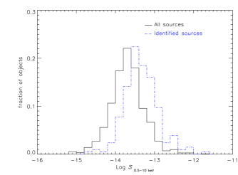
Figure 1: $S_{0.5-10\,{\rm keV}}$ distribution for the whole sample (solid line) and the sub-sample of identified sources (dashed-dot line).

Fig. 2 shows the redshift distributions of these sources. BLAGNs are detected up to redshifts of $\sim 3$, while at the flux limit of our optical identifications we do not detect NELGs and ALGs at redshifts above $\sim 0.5$. Similar distributions, at similar fluxes, have been found previously (e.g. Green et al. Green2004 (2004) for the ChaMP survey). In spite of the incomplete identifications, we do expect the identified sources to constitute a ”representative” sample of the underlying population of sources at X-ray fluxes above $\sim 2\times 10^{-14}{\rm erg\,cm^{-2}\,s^{-1}}$, where the identified fraction of objects is much higher ( 50%).

Figure 2: BLAGNs (solid line), NELGs (dashed line) and ALGs (dashed-dot line) redshift distributions.

3 Extraction of X-ray spectral products

We have cleaned the calibrated event files with the same filtering expressions that were used by the pipeline to create the EPIC X-ray images. This filtering removes time intervals contaminated by soft proton flares, cosmic ray tracks and spurious noise events not created by X-rays. For each object in the catalogue the SAS task region was used to define the source and background extraction regions.

The source region shape was defined as a circle centred on the source coordinates and with a typical radius of $\sim 14-30\arcsec$, depending on the source position within the detector. The background region was defined as an annulus centred at the source position, with inner radius equal to the source extraction radius and outer radius three times the inner radius. If there was overlap with nearby sources, the sizes of source and/or background regions were reduced to eliminate the overlap. If nearby sources were inside the background region their extraction regions were excluded from the background region.

Source and background spectra were then extracted with the SAS task evselect. Single and double events were included for the pn detector and single-quadruple events for the MOS detectors in the energy band 0.2-12 keV. Further, only events with the highest spectral quality (FLAG=0) were included for the EPIC-pn data.

In order to perform a proper spectral analysis, we created for each source the redistribution matrix file (RMF) and the ancillary response file (ARF), using the SAS tasks rmfgen and arfgen respectively. To maximise the signal to noise ratio, we have combined MOS1 and MOS2 source and background spectra and the corresponding response matrices. Merged source and background spectra were obtained by adding the individual spectra. Backscale values (size of the regions used to extract the spectra) and calibration matrices for the combined spectra were obtained weighting the input data with the exposure times.

For the fields with more than one observation, we added all the MOS and pn data for each epoch but MOS and pn data were not merged because of their different responses .

In order to permit the $\chi^{2}$ minimisation technique in the fitting process, the raw spectra were binned such that each bin contained $\geq 10$ counts (source plus background). We then imposed two quality thresholds on the grouped spectra selected for analysis: number of bins (MOS+pn) $\geq 5$, and number of background subtracted counts (MOS+pn) $\geq 50$.

This filtering process resulted in a final sample of 1137 sources having X-ray spectra of sufficient quality to analyse them individually (see Table 2 for the distribution of identified sources).

Figure 3: Distributions of background subtracted counts (MOS+pn) for the objects in our sample (solid histogram) and for the objects classified as BLAGNs or NELGs (shaded dot-dashed histogram). The vertical line indicates one of the quality thresholds applied to the spectra. For clarity, the last bin in the plots includes the spectra with more than 500 counts.

Figure 4: From top to bottom unfolded spectra of a) XMMU J221454.9-173949, absorbed BLAGN; b) XMMU J084132.3+704757, unabsorbed NELG ($\rm{L_{2-10\,keV}\sim 6\,10^{42}\,erg\,s^{-1}}$); c) XMMU J33106.2+241325, BLAGN with soft excess component (see Sect. 5.3 for details); d) XMMU J021908.3-044731, flat spectrum ($\Gamma=0.94_{-0.25}^{+0.23}$) object, still not identified.

Fig. 3 shows the quality of the selected spectra as a function of the 0.2-12 keV number of counts for the whole sample of sources (solid-line histogram) and for the objects identified as BLAGNs and NELGs (shaded histogram). The vertical line indicates the quality filter that we applied to select the spectra appropriate for the analysis. In Fig. 4 we present, as an example, the X-ray spectra of some of the objects that we have analysed.

4 Spectral Analysis

The data were fitted with the XSPEC (version 11.2) software package. The spectral analysis has been carried out fitting simultaneously MOS and pn spectra, forcing the models to have the same parameters in both instruments, including the normalisation (we do not expect significant calibration mismatches between instruments in the energy interval considered and for the quality level of our data).

We quantified the results of the spectral fits in terms of the null hypothesis probability ${\rm P(\chi^{2})}$ , i.e., the probability that the observed spectrum is derived from the parent model under scrutiny. We consider a model not good enough if ${\rm P(\chi^{2})}$ is less than 5%.

To test the significance of additional input parameters the F-test has been applied with an adopted significance threshold of 95%. As is shown in Protassov et al. Protassov2002 (2002), if the conditions to use the F-test statistic are not satisfied, the false positive rate might differ from the value expected for the selected confidence level. One of the conditions that must be satisfied, is that the null values of the additional parameters, should not be in the boundary of the set of possible values of the parameter. We are using the F-test to calculate the significance of detection of absorption, and one of the possible values of the absorbing column is zero. Hence, because one of the conditions for using the F-test is not satisfied, we do not know whether the fraction of spurious detections in our data differs from the 5% expected. To calculate this number, we carried out simulations of unabsorbed spectra, and then we calculated the number of cases where we detected absorption with a confidence level above 95%. We have detected absorption in $\sim$ 2% of the simulated spectra. As this fraction is not significantly different from the expected value, we decided to be conservative, and hence, we have continued with 5% as the number of spurious detections, or false positive rates.

4.1 Single power law (model A)

We have started the analysis fitting a single power law to the background-subtracted spectra, hereafter model A. This model has two free parameters, the normalisation and the continuum slope $\Gamma$. To account for the effect of the galactic neutral hydrogen absorption along the line of sight, a fixed photoelectric absorption component was included. The Galaxy H column density values for each field, ${\rm N_{H}^{Gal}}$, were extracted from the HI map of Dickey & Lockman (Lockman1990 (1990)). For the selected acceptance level, 139 (12%) objects had statistically unacceptable fits with this model, the expected number for the selected confidence level being 57. Within the sub-samples of identified sources, model A could not be accepted for 10 (7%) BLAGNs and 9 (31%) NELGs.

4.2 Single power law with excess absorption (model B)

Synthesis models of the XRB, based on AGN unification schemes (Setti & Woltjer Setti1989 (1989), Madau, Ghisellini & Fabian Madau1994 (1994), Comastri et al. Comastri1995 (1995), Pompilio, La Franca & Matt Pompilio2000 (2000), Gilli, Risaliti & Salvati Gilli2001 (2001)) predict a large population of highly absorbed AGNs. Hence we expect a significant fraction of our objects to exhibit absorption in excess of the Galactic value. An indication of absorption is to measure a flat spectral slope with model A. To study excess absorption, we fitted a model with two local absorbers, one with the column density fixed at the Galactic value and the other one as a free parameter ${\rm N_{H}^{obs}}$ (model B). Note that this last term is essentially indistinguishable from an absorber with column density $\sim{\rm N_{H}^{obs}\,(1+z)^{2.7}}$ (Barger et al Barger2002 (2002); Longair Longair1992 (1992)) at the redshift of the source, $z$, since absorption edges would not be detected in our highly grouped, moderate signal-to-noise spectra. This model has three free parameters, the normalisation, the continuum spectral slope $\Gamma$, and the equivalent absorbing column at $z=0$, ${\rm N_{H}^{obs}}$. The top panel in Fig. 5 compares the ${\rm P(\chi^{2})}$ distributions obtained with model A with the results from model B for the whole sample of sources. We see that the number of unacceptable fits has been reduced by a factor of $\sim 1.5$, implying the presence of intrinsically absorbed objects.

4.3 Single power law with intrinsic absorption (model C)

As an alternative, more physical parameterisation of the absorbing column of the BLAGN, NELG and ALG, we instead fitted photoelectric absorption at the redshift of the source (model C). The model has three free parameters, the normalisation, the continuum spectral slope, $\Gamma$, and the rest frame absorption, ${\rm N_{H}^{intr}}$. Fig. 5 compares the results of the fits obtained with model A and model C, for BLAGNs and NELGs. For a detailed description of the spectral properties of the 7 ALGs analysed, see Sec. 6. In the case of the BLAGNs, we did not find a substantial improvement in the overall quality of the fits, suggesting that the majority of the BLAGNs do not require intrinsic absorption in excess of the Galactic value. Therefore, for the statistically unacceptable fits, more complicated models might be needed to reproduce the spectra of these sources. On the contrary, the observed significant improvement in the quality of the NELG spectral fits obtained with model C, suggests that a large fraction of NELGs are intrinsically absorbed.

Figure 5: Comparison of the null hypothesis probability distributions, $P(\chi^{2})$, obtained from model A (simple power law, solid lines) and models B and C (observer frame absorbed power law and rest frame absorbed power law models, dashed lines). From top to bottom: whole sample of sources, BLAGNs and NELGs.

4.4 Absorbed power law and soft excess (model D)

The soft excess has been shown to be a common feature of the X-ray spectra of Seyfert 1 galaxies (Turner & Pounds Turner1989 (1989)). The physical origin of this emission is still unclear, since its determination depends on a knowledge of the shape of the power law and the quantity of absorption. It has been interpreted as primary emission from the accretion disc, gravitational energy released by viscosity in the disc, or as secondary radiation from the reprocessing of hard X-rays in the surface layers of the disc.

We have searched for soft excess among the BLAGNs and NELGs. We first have fitted their spectra with a power law and a low energy black body component at the redshift of the source, absorbed by the Galaxy. The soft excess emission, parameterised as a black body, adds to the model two parameters, the black body temperature and normalisation.

We have compared the $\chi^{2}$ of the fit with the values obtained with model A to search for the cases where the significance of a $\chi^{2}$ improvement was above 95%. From the 170 sources analysed (141 BLAGNs and 29 NELGs) we found evidence of soft excess emission in 12 sources ($\sim$7%), 10 BLAGNs and 2 NELGs.

As explained before, if soft excess is present in the spectra of the objects, it must be modelled properly to prevent the continuum spectral slope $\Gamma$ and/or the intrinsic absorption ${\rm N_{H}^{intr}}$ being incorrectly determined. Therefore we have analysed the X-ray spectra of these 12 sources in more detail. All the spectra have a large enough number of bins, 35$<$bins$<$317, to use a model with five free parameters: a power law and a low energy black body component, both absorbed by the Galaxy (${\rm N_{H}^{Gal}}$; fixed) and by absorption (${\rm N_{H}^{intr}}$; free) at the redshift of the sources (hereafter, model D). Results from this specific exercise are presented in Sect. 5.3.

5 Results of spectral fitting

5.1 The continuum shape

Although we know that a large fraction of sources in our list are absorbed, we have started the study with the results that we obtained with model A to allow comparison with spectral analyses of data with low signal to noise. This model, as was explained before, does not take into account the effects of absorption or soft excesses.

To calculate the objects average photon index, $\langle\Gamma\rangle$, we have used the standard formula for the weighted mean,

$$\langle\Gamma\rangle=\sum\,P_{i}\times\,\Gamma_{i}$$

where the weight, $P_{i}$, of each individual best fit value, $\Gamma_{i}$, is a function of the error obtained from the fit, $\sigma_{i}$,

$$P_{i}={1\,/\sigma_{i}^{2}\over\sum\,(1\,/\sigma_{i}^{2}\,)}$$

To calculate the uncertainty in $\langle\Gamma\rangle$ we have used the standard deviation (Bevington Bevington1992 (1992))

$$\sigma^{2}={1\over(\rm{N}-1)}\,\sum\,P_{i}\times(\Gamma_{i}-\langle\Gamma\rangle)^{2}$$

that includes the measurement errors, $\sigma_{i}$, and the dispersion of each $\Gamma_{i}$ from the estimated value $\langle\Gamma\rangle$.

Following these definitions, we find our sources to have a continuum emission, from 0.2 to 12 keV, with an average slope of $\langle\Gamma\rangle=1.86\pm 0.02$ (the arithmetic mean being $1.70\pm 0.02$). To study the dependence of the objects average spectrum on the X-ray flux, we have calculated the values of $\langle\Gamma\rangle$ in bins of 0.5-2 and 2-10 keV flux (each bin containing the same number of objects). Fig. 6 shows the results that we have obtained. We see that the average spectrum of the sources becomes harder with decreasing 0.5-2 keV flux, with $\langle\Gamma\rangle$ going from $2.01\pm 0.03$ at $\sim 4.4\times 10^{-14}\,\mathrm{erg\,cm}^{-2}\mathrm{s}^{-1}$ to $0.95\pm 0.12$ at $\sim 10^{-15}\,\mathrm{erg\,cm}^{-2}\,\mathrm{s}^{-1}$. This trend (harder sources at fainter 0.5-2 keV fluxes) has been found in previous X-ray spectral analyses (e.g., Vikhlinin et al. Vikhlinin1995 (1999), Mittaz et al. Mittaz1999 (1999), Tozzi et al. Tozzi2001 (2001), Mainieri et al. Mainieri2002 (2002)). Its origin is still not clear, although it could be explained as a rapid increase in the intrinsic absorption of the objects with decreasing flux, as it is predicted by some AGN synthesis models (see Gilli et al. Gilli2001 (2001))
It is not possible to see the same effect using the 2-10 keV fluxes, where $\Gamma$ seems to become softer at fainter fluxes (see Fig. 6). It is important to note that this softening of $\Gamma$ is not a real property of our objects. It comes from using different energy bands simultaneously in the source detection. As we go to fainter 2-10 keV fluxes, it is more difficult to detect sources with flat spectral slopes (hard objects) because their spectra peak at energies above $\sim$ 2 keV where we know the sensitivity of the X-ray detectors decreases rapidly. Hence, the number of objects only detected in the soft band becomes more important at fainter 2-10 keV fluxes, specially below $\sim 2\times 10^{-14}\,{\rm erg\,cm^{-2}\,s^{-1}}$. Note that the last bin at the faintest fluxes (see Fig. 6) is located at a value of $\langle\Gamma\rangle$ of more than 2.5. The objects that contribute to this bin have spectra with very few counts and therefore the values of $\Gamma$ are poorly constrained.

Figure 6: Weighted photon index versus $S_{0.5-2\,{\rm keV}}$ and $S_{2-10\,{\rm keV}}$ from model A (simple power law). The results obtained for the objects with X-ray spectra with more than 150 counts (background subtracted) are included for comparison. Error bars correspond to 90% confidence

We have studied in more detail whether the observed hardening of $\Gamma$ with decreasing soft flux could be affected by any bias introduced during our analysis. We first have checked that the same result is obtained when only sources with more than 150 counts (circles in Fig. 6) are used. Therefore, the sources with poor spectral quality are not introducing any bias in our result.

We expect the majority of the observations that we have used, not to be deep enough as to detect sources with a 0.5-2 keV flux of ${\rm\sim 10^{-15}\,erg\,cm^{-2}\,s^{-1}}$ in the soft band. Hence, it could be possible that our $\langle\Gamma\rangle$ becomes harder with decreasing flux partly due to the contribution to each bin from bright hard sources not detected in the soft band. This can be checked by repeating the plot of Fig. 6 with those sources selected in the soft or hard bands (detection likelihoods above 10 on each band). The results, plotted in Fig. 7, show a very similar dependence of $\Gamma$ with flux. Only the $\langle\Gamma\rangle$ of the bin at the faintest soft fluxes in Fig. 6, could be affected or even dominated by the contribution of bright hard sources not detected in the soft band. It is interesting to note that the hardening of $\Gamma$ is more important for objects detected in the 2-10 keV band (see Fig. 7). If absorption is producing the hardening of $\Gamma$, this result suggests that we are seeing the same population of objects in the soft and hard bands, the only difference being that the objects detected in the 2-10 keV band are more absorbed on average.

Figure 7: Weighted photon index versus $S_{0.5-2\,{\rm keV}}$ from model A (simple power law) for sources with detection likelihood $\geq$10 in the 0.5-2 keV band (squares) and for sources with detection likelihood $\geq$10 in the 2-10 keV band (circles). Error bars correspond to 90% confidence

Finally we have used the source detection efficiency function, W($\Gamma,{\it S}$) (see Appendix  A), to correct our results for all the biases of our study. The de-biased average values of $\Gamma$ at each bin of flux were obtained weighting each individual value, $\Gamma_{i}$ with the function:

$$P_{i}={1\,/(\sigma_{i}^{2}\times W(\Gamma_{i},{\it S_{i}}))\over\sum\,1\,/(\sigma_{i}^{2}\times W(\Gamma_{i},{\it S_{i}}))}$$

where the sum is calculated with all the sources falling in the specified bin in the $\Gamma$, S plane (for a detailed explanation see Appendix  A).

The results are shown in Fig. 8, the left plot for the whole sample of sources, and the right plot for the sources detected in the soft band. For comparison we have calculated the $\langle\Gamma\rangle$ values weighted with the fitting errors in the same flux bins (stars in the plots). We still see the hardening of $\langle\Gamma\rangle$ with the 0.5-2 keV flux, so this dependence is indeed a real property of the population of the sources analysed.

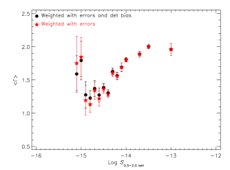
Figure 8: Comparison of the weighted photon index versus $S_{0.5-2\,{\rm keV}}$ from model A (simple power law) with the values obtained after correcting for the source list biases. Left for the whole sample of objects and right for the sub-sample of sources with detection likelihood $\geq$10 in the 0.5-2 keV band. Error bars correspond to 90% confidence

5.2 Excess Absorption

The fit to the X-ray spectra with a single power law (model A) yields a large number of sources with statistically unacceptable fits. Models B and C reduce significantly the number of unacceptable fits as it is shown in Fig. 5, suggesting that a substantial fraction of our sources could be X-ray absorbed, in agreement with the predictions of the standard synthesis models of the XRB (Comastri et al. Comastri1995 (1995), Gilli et al Gilli2001 (2001)).

To search for absorbed objects we used the F-test, measuring the improvement in the $\chi^{2}$ of the fits after adding absorption to the model. A 95% confidence cutoff is adopted for absorption to be detected. In Table 3, we show the total number of objects of different types, the number of absorbed objects of that type, and the fraction of absorbed objects of each type with its uncertainty and significance.

For a sample of $N$ objects, of which $n$ are absorbed, the Bayesian posterior probability of the fraction of absorbed objects is $P(f)\propto(f+f_{spu})^{n}(1-f-f_{spu})^{N-n}$ (from the binomial distribution), where $f_{spu}$ is the fraction of spurious detections (for our sources 5%). We used the mode of P(f) to estimate the fraction (corrected from spurious detections) of absorbed objects within each class of sources. The errors in the fractions were calculated integrating P(f) from the mode value in the two directions until we obtained 45% of the probability (90% errors). For every “class” of sources, we measured the confidence of detection of absorption integrating the P(f) distributions from f=1 down to the value where the integral is equal to 0.9973 (or 3$\sigma$). These values, listed in the last column of Table 3, indicate the fraction of absorbed objects that we have detected within each class of sources with a significance of more than 3$\sigma$. For example, we know with a confidence of more than 3$\sigma$ that at least $\sim$ 1% of BLAGNs and $\sim$ 17% of NELGs are absorbed.

It appears that the fraction of absorbed objects varies substantially among different classes of object, with the NELGs having the highest fraction. We have used the method described in Stevens et al. Stevens2005 (2005) to study whether our samples of BLAGNs and NELGs have different fractions of absorbed objects. Assuming that BLAGNs and NELGs come from the same parent population, the fraction of absorbed objects is

$$P(f)\propto(f+f_{spu})^{(n+m)}(1-f-f_{spu})^{(N+M-n-m)}$$

where M and N are the number of sources in the two samples and m and n the number of detections on each sample.

The probability of detection of i objects in the first sample and j in the second one is given by

$$P(i,j;N,M)={M\choose j}{N\choose i}\,\int_{0}^{1}\,df\,P(f)\,(f+f_{spu})^{(i+j)}$$

$$\,\,\,\,\,\,\,\,\,\,\,\,\,\,\,\,\,\,\,\,\,\,\,\,\,\,\,\,\,\,\,\,\,\,\,\,\times\,\,\,(1-f-f_{spu})^{(N+M-i-j)}$$

The fractions of absorbed objects in BLAGNs and NELGs will be different if the probability of detecting $\leq m$ in the first sample and $\geq n$ in the second one is low, i.e. if $P(\geq n,\leq m;N,M)=\sum_{j=0}^{M}\sum_{i=n}^{N}P(i,j;N,M)$ is low. We find that $P(m\leq 16,n\geq 13;141,29)=0.000013$. Therefore we see that the fraction of absorbed objects in BLAGNs and NELGs is different with a significance of more than 3$\sigma$. We cannot distinguish the fraction of absorbed objects among NELGs and ALGs (the probability of them being different is not significant).

Figure 9: Distributions of intrinsic absorption for BLAGNs (solid histogram) and NELGs (dashed histogram).

Fig. 9 shows the intrinsic ${\rm N_{H}^{intr}}$ distributions measured for the absorbed BLAGNs and NELGs. BLAGNs show column densities $4.5\times 10^{20}<{\rm N_{H}^{intr}}<2.3\times 10^{22}\,{\rm cm}^{-2}$ while NELGs seem to cover a much wider range of absorption, with $1.1\times 10^{21}<{\rm N_{H}^{intr}}<1.7\times 10^{23}\,\mathrm{cm}^{-2}$. However, the small number of objects does not allow us to find a significantly different (in terms of the Kolmogorov-Smirnov test) distribution of absorbing columns between BLAGNs and NELGs.

Figure 10: Photon index versus intrinsic absorption for absorbed (F-test significance $\geq 95\%$) BLAGNs (triangles) and NELGs (diamonds).

To be confident that the detected intrinsic absorptions among identified sources were not affected by the quality of their spectra, we have plotted $\Gamma$ versus ${\rm N_{H}^{intr}}$ to search for any correlation between the two spectral parameters. Such a correlation would be expected if the detections of absorption were spurious and linked to very large values of $\Gamma$. The results are shown in Fig. 10. The plot shows no apparent correlation between $\Gamma$ and ${\rm N_{H}^{intr}}$.

A Kolmogorov-Smirnov comparison between the redshift distributions of unabsorbed and absorbed BLAGNs does not indicate a significant difference between the two. The same result is obtained when comparing the 2-10 keV luminosity distributions of absorbed and unabsorbed BLAGNs and NELGs (we use the 2-10 keV energy band because it is less affected by absorption). We conclude that X-ray absorption does not occur preferentially at any particular redshift (in BLAGNs) or X-ray luminosity.

Finally, we have tested whether the lack of optical broad emission lines in unabsorbed NELGs can be explained in terms of AGN/host galaxy contrast (Lumsden et al. Lumsden2001 (2001), Moran et al. Moran2002 (2002), Page et al. Page2003 (2003), Severgnini et al. Severgnini2003 (2003)) . To this end, we have compared the 2-10 keV luminosity distributions of two sub-samples of unabsorbed BLAGNs and NELGs detected with redshifts ranging from 0.17 to 0.7, where the redshift distributions of BLAGNs and NELGs overlap (see Fig. 2). The Kolmogorov-Smirnov significance of the two distributions being different is $\sim$ 99%. Furthermore, the average luminosities of the selected BLAGNs and NELGs were found to be 43.7$\pm$0.16 and 43.2$\pm$0.11 (in log units). Therefore, we have seen that our unabsorbed NELGs are on average significantly less luminous than unabsorbed BLAGNs at similar redshifts, and hence, our data are consistent with the explanation of non detection of broad optical lines in unabsorbed NELGs as an AGN/ host-galaxy contrast effect.

Table 3: Fractions of F-test absorbed objects and significances.

Type	${\rm N_{tot}}$	${\rm N_{abs}}$	${\it f_{-}^{+}}^{\mathrm{a}}$	${\rm F^{\mathrm{b}}}$
All	1137	245	$0.17\,_{-0.02}^{+0.02}$	0.1335
BLAGNs	141	16	$0.06\,_{-0.04}^{+0.05}$	0.0089
NELGs	29	13	$0.40\,_{-0.14}^{+0.15}$	0.1740
ALG	7	3	$0.40\,_{-0.20}^{+0.20}$	0.0400

• The f values are the mode of the function P(f) (see Sec. 5.2 for details). The errors are 90$\%$

• F is where P(f $\geq$ F)=0.9973 (3$\sigma$)

5.3 Soft excess

We have previously shown that $\sim$7% of the sources identified as BLAGNs or NELGs exhibit significant soft excess emission. To measure the broad band spectral parameters of these sources, and in particular the underlying power law index $\Gamma$ we have used model D, as described in detail in Sec. 4.

Table 4: Spectral parameters of sources with a soft excess component detected

$$\begin{array}[]{c c c c c c c c c c c c}\hline\cr\vskip 3.0pt plus 1.0pt minus 1.0pt\cr\mathrm{Name\,^{{\rm a}}}&\mathrm{Class}&\mathrm{redshift}&\Gamma_{-}^{+}&\mathrm{N_{H}^{intr}}\,^{\mathrm{b}}&\mathrm{kT_{-}^{+}}&\mathrm{{\it S}_{0.5-2}}&\mathrm{L_{0.5-2}}&\mathrm{model\,C}\,^{\mathrm{c}}&\mathrm{model\,D}\,^{\mathrm{d}}\\ &&&&(10^{20}\,\mathrm{cm}^{-2})&\mathrm{(keV)}&(\%)&(\%)&\\ \vskip 3.0pt plus 1.0pt minus 1.0pt\cr\hline\cr\hline\cr\vskip 3.0pt plus 1.0pt minus 1.0pt\cr\mathrm{XMMU\,J001831.7+162924}&\mathrm{BLAGN}&0.551&2.35_{-0.18}^{+0.17}&4.15_{-2.37}^{+11.25}&0.186_{-0.126}^{+0.259}&15.95&23.39&\mathrm{Not\,\,\,abs.}&\mathrm{abs.}\\ \mathrm{XMMU\,J021808.2-045844}&\mathrm{BLAGN}&0.712&2.08_{-0.05}^{+0.04}&<10^{20}&0.142_{-0.111}^{+0.164}&6.55&19.49&\mathrm{Not\,\,\,abs.}&\mathrm{Not\,\,\,abs.}\\ \mathrm{XMMU\,J021830.5-045622}&\mathrm{BLAGN}&1.430&2.28_{-0.18}^{+0.10}&<10^{20}&0.129_{-0.082}^{+0.223}&1.89&30.08&\mathrm{Not\,\,\,abs.}&\mathrm{Not\,\,\,abs.}\\ \mathrm{XMMU\,J061728.6+710600}&\mathrm{BLAGN}&0.219&1.68_{-0.37}^{+0.56}&<10^{20}&0.214_{-0.111}^{+0.253}&39.54&44.57&\mathrm{Not\,\,\,abs.}&\mathrm{Not\,\,\,abs.}\\ \mathrm{XMMU\,J061730.9+705955}&\mathrm{NELG}&0.200&2.02_{-1.00}^{+1.13}&<10^{20}&0.207_{-0.142}^{+0.272}&44.14&49.31&\mathrm{abs.}&\mathrm{Not\,\,\,abs.}\\ \mathrm{XMMU\,J074311.9+742935}&\mathrm{BLAGN}&0.332&2.05_{-0.05}^{+0.03}&<10^{20}&0.119_{-0.106}^{+0.130}&12.22&22.12&\mathrm{Not\,\,\,abs.}&\mathrm{Not\,\,\,abs.}\\ \mathrm{XMMU\,J12226.1+752616}&\mathrm{NELG}&0.238&1.82_{-0.10}^{+0.14}&11.17_{-2.30}^{+2.43}&0.146_{-0.112}^{+0.208}&12.30&22.72&\mathrm{abs.}&\mathrm{abs.}\\ \mathrm{XMMU\,J13316.2+241326}&\mathrm{BLAGN}&0.174&1.83_{-0.26}^{+0.45}&<10^{20}&0.085_{-0.064}^{+0.116}&14.71&25.20&\mathrm{Not\,\,\,abs.}&\mathrm{Not\,\,\,abs.}\\ \mathrm{XMMU\,J212904.5-154448}&\mathrm{BLAGN}&0.431&1.29_{-0.36}^{+0.27}&14.21_{-5.81}^{+32.59}&0.205_{-0.142}^{+0.251}&54.55&72.74&\mathrm{Not\,\,\,abs.}&\mathrm{abs.}\\ \mathrm{XMMU\,J221515.1-173224}&\mathrm{BLAGN}&1.165&2.06_{-0.35}^{+0.37}&<10^{20}&0.212_{-0.192}^{+0.233}&24.75&49.69&\mathrm{Not\,\,\,abs.}&\mathrm{Not\,\,\,abs.}\\ \mathrm{XMMU\,J221523.6-174321}&\mathrm{BLAGN}&0.956&2.15_{-0.23}^{+0.17}&<10^{20}&0.112_{-0.021}^{+0.234}&1.86&19.16&\mathrm{Not\,\,\,abs.}&\mathrm{Not\,\,\,abs.}\\ \mathrm{XMMU\,J222823.6-051306}&\mathrm{BLAGN}&0.758&1.52_{-0.15}^{+0.14}&15.61_{-7.20}^{+12.39}&0.262_{-0.171}^{+0.379}&35.78&54.55&\mathrm{Not\,\,\,abs.}&\mathrm{abs.}\\ \vskip 3.0pt plus 1.0pt minus 1.0pt\cr\hline\cr\end{array}$$

• XMM-Newton source name

• Intrinsic absorption measured with model D

• Detection of intrinsic absorption with model C (F-test comparison of the $\chi^{2}$ from model A and model C)

• Detection of intrinsic absorption with model D (F-test comparison of the $\chi^{2}$ from model A and model D)

The results of the fits are listed in Table 4, where for each source we have included its IAU-style XMM-Newton source name, the optical classification, redshift, and the spectral parameters measured with model D. We have also included the soft excess contributions to the flux and luminosity in the soft band and the F-test results obtained from the comparison of $\chi^{2}$ from model A to $\chi^{2}$ from model C and model D. We now discuss some particular sources in detail:

XMMU J001831.7+162924, XMMU J222823.6-051306, XMMU J212904.5-154448: we obtained an improvement in the spectral fits with model C, but the F-test significance was in all cases below 95%, therefore the sources were classified as unabsorbed. A proper modelling of the soft excess emission with model D allowed us to find significant absorption above the Galactic value in all the sources.

XMMU J221515.1-173224: we obtained an unusually steep spectral slope with model A, $\Gamma=2.67_{-0.06}^{+0.05}$. The quality of the fit did not improve significantly with model C. With model D we obtained a significant improvement in the fit ($>99.99\%$). This model did not require absorption in excess of the Galactic value . The measured temperature of the soft excess emission was kT=$0.05_{-0.01}^{+0.03}$, below the typical values found for the rest of the sources. The fitted continuum was still significantly steep, with $\Gamma=2.60_{-0.11}^{+0.04}$.We tried to find a more typical value of $\Gamma$ fitting the continuum slope at high energies ($>2$ keV) with model A. We obtained a value of $\Gamma$ significantly lower, $2.06_{-0.35}^{+0.37}$ and in agreement with the average spectral slopes observed in unabsorbed AGN. With $\Gamma$ fixed to the above value the fit did not improve with model C, but with model D we still obtained an F-test significance of $>99.99\%$. The model did not require absorption in excess of the Galactic value, therefore we believe the improvement is due entirely to the soft excess component. We adopted this model as the best fit model for the source although the $\chi^{2}$ of the fit was slightly worse that the value obtained with $\Gamma$ fully variable.

XMMU J061730.9+705955: we found a significant column density with model C, hence the source was classified as absorbed. However we obtained a very steep spectral slope, $\Gamma=2.87_{-0.31}^{+0.35}$. With model D we obtained a better fit of the data and more typical values for the spectral parameters, although model D did not require intrinsic absorption. We have chosen model D in preference to model C for this source.

It is interesting to note that for some of the sources that we have analysed, we found very flat spectral slopes with model A, but they all required significant quantities of soft excess emission. This is the case for XMMU J12226.1+752616 and XMMU J222823.6-051306, with measured model A spectral slopes of $\Gamma=1.52_{-0.04}^{+0.04}$ and $\Gamma=1.78_{-0.11}^{+0.11}$ respectively.

5.4 Results from best fit model

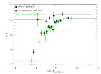
Figure 11: $\langle\Gamma\rangle$ versus $S_{0.5-2\,{\rm keV}}$ obtained from the best fit model of each object. Squares denote the whole sample; stars absorbed sources (F-test$\geq 95.0\%$) and triangles unabsorbed sources (F-test$<95.0\%$).

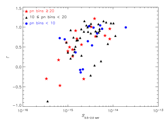
Figure 12: $\Gamma$ versus $S_{0.5-2\,{\rm keV}}$ for objects with flat spectrum ($\Gamma$ positive error bar $<$1.5). We have grouped the objects in terms of the number of bins in their pn spectrum.

To test whether the spectral hardening observed using model A is due to an increase in intrinsic absorption at the faintest fluxes, we compared $\Gamma$ (from the best fit model in terms of the F-test results) to the soft X-ray flux for each source. The best fit model can be model A or model B for the unidentified sources, and model A or model C for the identified sources (or model D for BLAGNs and NELGs when soft excess emission was detected). Using the best fit model for each object we obtained a value of $\langle\Gamma\rangle=1.96\pm 0.01$ (the unweighted value was $2.08\pm 0.04$). The dependence of $\langle\Gamma\rangle$ with the soft flux is plotted in Fig. 11, where we see that:

1. The average continuum of absorbed sources is significantly softer than the continuum of unabsorbed sources, especially at the faintest fluxes, with $\langle\Gamma\rangle=2.15\pm 0.04$ (the unweighted value being $3.12\pm 0.12$) for the absorbed sources and $\langle\Gamma\rangle=1.94\pm 0.01$ (the unweighted value being $1.79\pm 0.02$) for the unabsorbed sources.

2. There is no hardening of the average spectral slope for the absorbed sources. The hardening of $\Gamma$ seen in these objects when fitted with the SPL model is likely to be an effect of absorption only.

3. For the sources where absorption was not detected in terms of the F-test, we still observe a significant hardening of the average spectral slope with the X-ray flux.

Since the sources where absorption is detected do not exhibit any significant variation of the underlying spectral index with flux, does this hold true for the remaining sources? We first wanted to check whether any effect could lead to an apparent flattening of the spectral shape towards fainter fluxes when absorption is included in the fitting model. To this goal, we have generated a number of fake spectra with an underlying power law $\Gamma=2$ at various fluxes spanning those of our sample, and different amounts of absorption at $z=0$.

We have then first fitted these spectra with models A and B, and then we have compared the $\chi^{2}$ of the fits with the F-test. We found a range of low values of ${\rm N_{H}^{obs}}$ where absorption was not significantly detected when model A was replaced by model B (F-test $<$ 95%). In these cases, the best fit value of $\Gamma$ ( i.e., the value obtained with model A) was indeed lower than the input one, and it can reach values in the range $\Gamma\sim$1-2.

A second result of this exercise is, if we hold the absorption in the simulated spectra but vary the flux, at fainter fluxes the typical values of $\Gamma$ fitted are marginally harder than at higher fluxes (and then fitted values of ${\rm N_{H}}$ tend to be lower than the input ones). We believe this effect to be due to a degradation of the spectral resolution of the X-ray spectrum, produced by the necessary grouping in very wide bands to achieve the desired statistics (10 counts/bin). This leads, in particular, to a smoothing of the model count rate function (which is the effective area times the input spectrum, convolved with the redistribution matrix) in the whole spectral range, but in particular in the vicinity of its peak at soft energies where most of the counts are detected. This produces an undesired slight hardening of the spectrum.

However, this effect is unlikely to produce the hardening of the unabsorbed sources that we see. The reason is that in this case we should see the lowest quality spectra (i.e., those with the smaller number of bins) being more prone to this effect, but this is not the case. Fig. 12 shows the sources that we detect in the real sample with flat spectra (best fit $\Gamma$ error bar upper limit below 1.5), grouped in terms of the number of bins in their EPIC-pn spectra. We clearly see that the hardening is not correlated with the quality of the spectra, and therefore the above effect does not dominate.

We conclude that the hardening towards fainter fluxes is real. This still leaves two options for its origin: intrinsic flattening of the power law or undetected low level absorption. Although the current data do not allow us to distinguish between them, there is nothing inconsistent with the simplest hypothesis which is that these sources are absorbed at a level which is undetectable in the current data.This is also supported by the results of Fig. 6 (right plot) where we do not see hardening of $\Gamma$ with the 2-10 keV flux down to $\sim 2\times 10^{-14}{\rm erg\,cm^{-2}\,s^{-1}}$. If absorption is producing the hardening effect that we see in our objects, then we do not expect to see the same effect using 2-10 keV fluxes, because they are less affected by absorption. However, deeper observations are needed to assess this point for sources at fluxes similar to those of the sources in our sample. The results of a detailed X-ray spectral analysis of the sources that were detected with XMM-Newton in a deep observation in the Lockman Hole field will be published in Mateos et al. Mateos2005 (2005) (in preparation).

The average spectral indices for the best fit model in the sub-samples of BLAGNs and NELGs are $1.99\pm 0.02$ and $2.35\pm 0.09$, both in agreement with the canonical value measured for nearby unabsorbed BLAGNs (Nandra & Pounds Nandra1994 (1994)). Both sub-samples of sources exhibit the same dependence with the soft X-ray flux as shown in Fig. 13. We still detect a clear correlation between the spectral slope and the soft X-ray flux.

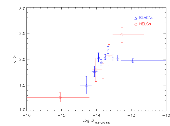
Figure 13: $\langle\Gamma\rangle$ from best fit model versus $S_{0.5-2\,{\rm keV}}$ for BLAGNs (triangles) and NELGs (circles). The hardening of the spectral slope is evident even among the sub-samples of AGNs. Error bars correspond to $90\%$ confidence level.

Table 5: Comparison of the weighted mean spectral photon index obtained for different types of sources with the values from the Maximum Likelihood analysis. The best fit spectral slopes for each object were used in the calculations.

$$\begin{array}[]{l c c c c c}\hline\cr\vskip 3.0pt plus 1.0pt minus 1.0pt\cr&\lx@intercol\hfil\rm{Maximum}\hfil\lx@intercol&{\rm{Weighted}}\\ &\lx@intercol\hfil\rm{Likelihood}\hfil\lx@intercol&{\rm{Mean}}\\ {\rm Sample}&\langle\Gamma\rangle&\sigma&\langle\Gamma\rangle\\ \vskip 3.0pt plus 1.0pt minus 1.0pt\cr\hline\cr\hline\cr\vskip 3.0pt plus 1.0pt minus 1.0pt\cr{\rm Whole\,\,sample}&1.86\,_{-0.03}^{+0.02}&0.36\,_{-0.04}^{+0.01}&1.96\pm 0.01\\ {\rm BLAGN}&1.98\,_{-0.04}^{+0.04}&0.21\,_{-0.04}^{+0.05}&1.99\pm 0.02\\ {\rm NELG}&1.85\,_{-0.17}^{+0.16}&0.36\,_{-0.10}^{+0.14}&2.35\pm 0.09\\ \vskip 3.0pt plus 1.0pt minus 1.0pt\cr\hline\cr\end{array}$$

5.5 Photon index intrinsic dispersion

Figure 14: Contour diagrams for the average spectral slope and intrinsic dispersion of our objects obtained from the Maximum Likelihood analysis (see Sec. 5.5). The spectral slopes obtained from the best fit model were used in the calculations. Solid line for BLAGNs and dashed line for NELGs. The contours are defined as $\Delta\chi^{2}$=2.3, 6.17 and 11.8 corresponding to standard 1,2 and 3$\sigma$ confidence regions for two parameters.

In all the above analysis we have observed a clear dispersion in the measured spectral slope of our objects, even within the sub-samples of BLAGNs and NELGs, with the largest scatter in $\Gamma$ being observed for the NELGs. To test whether the observed scattering is intrinsic to the sources we have followed the procedure described in Nandra & Pounds (Nandra1994 (1994)) and Maccacaro et al. (Maccacaro1988 (1988)), where the distribution of source spectral indices is assumed to be well reproduced by a Gaussian distribution of mean $\langle\Gamma\rangle$ and dispersion $\sigma_{\langle\Gamma\rangle}$. The best estimates of $\langle\Gamma\rangle$ and $\sigma_{\langle\Gamma\rangle}$ are obtained with the maximum likelihood (ML) technique. We have calculated the distribution of the spectral slopes that we obtained from the best fit model for the whole sample and the sub-samples of BLAGNs and NELGs. The results are shown in Table 5. In all the classes we measured a significant dispersion in spectral slopes. The large error in $\Gamma$ obtained for NELGs did not allow us to differentiate the average spectral index of NELGs from that of BLAGNs. We see that the mean values of $\Gamma$ computed with the ML and the weighted mean are very different, in particular for the NELGs. The reason is that with the ML method objects with untypical $\Gamma$ (i.e. outliers) and not very large errors will increase the dispersion of the fitted gaussian distribution rather than significantly affecting the mean.

Our results do not show any trend in the underlying power law of the NELGs to be harder than that of the BLAGNs even at the faintest fluxes. Previous results based on $ROSAT$ data (see Almaini et al Almaini1996 (1996), Romero-Colmenero et al. Romero1996 (1996)) do find a flatter average spectral slope for NELGs ($\sim 1.5$) than for BLAGN ($\sim 2$). Our data shows that the spectral differences between these two classes of sources are due mostly (if not totally) to differing amounts of absorption rather than to differences in the underlying power law spectra. Therefore many objects classified as NELGs may contain active nuclei.

Fig. 14 shows the $\langle\Gamma\rangle$ versus $\sigma_{\langle\Gamma\rangle}$ contour diagrams for the sub-samples of BLAGNs (solid lines) and NELGs (dashed lines), clearly showing the existence of an intrinsic dispersion in $\Gamma$ with a confidence of more than 3$\sigma$.

5.6 Spectral cosmic evolution

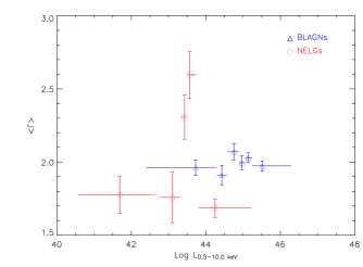
Figure 15: Weighted $\langle\Gamma\rangle$ versus ${\rm L}_{0.5-10\,{\rm keV}}$ for BLAGNs (triangles) and NELGs (circles). Error bars correspond to $90\%$ confidence level.

Figure 16: $\langle\Gamma\rangle$ versus redshift for BLAGNs. We have used the values of $\Gamma$ from the best fit model for each object (i.e. with absorption and soft excess if required). Error bars correspond to $90\%$ confidence level.

No correlation was found between $\Gamma$ and the rest-frame 0.5-10 keV luminosities, as shown in Fig. 15. For the sub-sample of BLAGNs we studied the measured $\Gamma$ that we obtained from each best fit model as a function of the redshift, but we did not find any clear tendency between the two parameters as can be seen in Fig. 16.

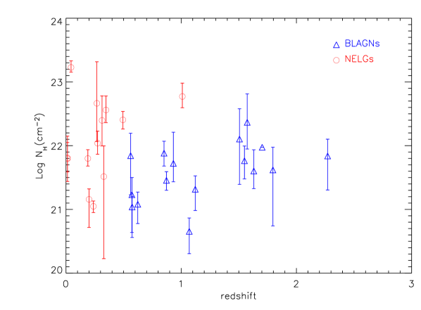
Figure 17: Intrinsic absorption as a function of redshift for absorbed (F-test significance $\geq$95%) BLAGNs (triangles) and NELGs (circles).

We have studied the redshift distribution of the measured rest frame absorbing column densities for the absorbed sub-samples of BLAGNs and NELGs. The results, shown in Fig. 17, show no evidence of evolution of ${\rm N_{H}^{intr}}$ with redshift. However, the ranges of the 2-D parameter space that we fully sample with our source list are unclear.

We expect the minimum detected absorption to increase with $z$. This can be easily explained in terms of absorption being redshifted towards lower energies and further decreased by a factor $(1+z)^{2.7}$ as we move upwards in $z$.

To study if there exists a maximum detected column (only the brightest sources being actually detectable when heavy absorption is present), and if this limit depends on redshift, we have carried out simulations as follows. A 3-D parameter space was defined with the axes being redshift, luminosity and intrinsic (rest-frame) absorption. For each parameter we have defined a grid of values covering the observational limits established by our sources. First, for each point in the ${\rm N_{H}^{intr}}$-$z$ plane we simulate a spectrum for each BLAGN or NELG source in our sample, using its spectral response matrices and exposure time and assuming $\Gamma=2$. As explained in Sec. 3 we have only analysed those spectra with more than 50 counts (background subtracted). We use this limit to calculate the required minimum luminosity for each source to fulfil this constraint. Luminosities lower than this one would produce a spectrum outside our quality bounds.

Second, for a number of luminosities above this limit (still, for each value of intrinsic absorbing column and $z$) we simulate a spectrum for every source. These spectra were analysed following the same procedure that we used for the real spectra giving a full coverage of the above 3-D parameter space.

We then examined the fitted values of ${\rm N_{H}^{intr}}$ as a function of redshift $z$ for a range of luminosities. The simulations confirm that the minimum detection of absorption depends strongly on $z$ for the reason explained above. We also found two limits to the maximum absorption detected as a function $z$. The first one is the source detection itself: heavy absorption reduces significantly the flux of the source and makes detection very difficult, especially at high redshifts. The second limit is the detection of absorption: even if the source is detected, if its luminosity is not high enough we will measure an absorption below the maximum value established by the detection limit.

This strong dependence on luminosity and redshift makes it very difficult to derive the real absorbing column distribution in terms of the fitted values. The best way we found to tackle this problem is to compare our results with the predictions of specific models for the distribution of absorbing columns, folding the input values through the same effects as the real data. This is discussed in Sect. 7 in the framework of unified AGN models for the XRB.

6 ALGs X-ray spectra

The objects with galaxy-like optical spectra not showing emission line signatures were classified as absorption line galaxies (ALG).

The inferred high X-ray luminosities obtained from the analysis of their X-ray spectra strongly suggests that an AGN is the source of the X-ray emission in at least 5 out of the 7 objects. The peculiar properties of these objects have been explained by a very high column density that would be obscuring the AGN broad and narrow line regions. This hypothesis has found observational support, because many of the ALGs studied have been found to be X-ray obscured (Mainieri et al. Mainieri2002 (2002), Comastri et al. Comastri2002 (2002)). However there are several examples of ALGs for which the obscuration model does not apply. In these cases other possible explanations have been suggested, e.g. that a BL Lac could be present in the core of some ALGs (Brusa et al. Brusa2003 (2003)). Alternatively some objects might host an AGN with a non-standard accretion disk (Yuan & Narayan Yuan2004 (2004)). A final possibility is that some ALGs may have normal (unabsorbed) AGNs that could be hidden if the host galaxy is bright enough (Severgnini et al. Severgnini2003 (2003), Page et al. Page2003 (2003)).

We now describe the X-ray spectral properties of the ALGs found in our list:

XMMU J122017.7+752216 is an optically normal galaxy that looks extended in the X-ray image. Its soft X-ray emission is best reproduced with a thermal model with temperature $k\rm{T=0.64_{-0.04}^{+0.04}}$ keV and metallicity $Z=Z\odot$. The fit does not improve leaving $Z$ as a free parameter. However, the high energy X-ray spectrum is best modelled with an unabsorbed power law of spectral slope $\Gamma=1.87_{-0.11}^{+0.12}$. We cannot confirm whether the source of the hard X-ray emission is an AGN due to the low value of the hard X-ray luminosity inferred from this model ($\rm{L_{2-10}=3.1\times 10^{39}erg\,s^{-1}}$).

The nature of XMMU J021822.1-050612 was studied in detail by Severgnini et al. (Severgnini2003 (2003)). They found the X-ray spectrum to be best modelled with an absorbed power law.

The X-ray spectra of XMMU J010320.2-064157 and XMMU J084211.6+710145 were best reproduced with an obscured (F-test values 99.7% and 95.0%) AGN with $\Gamma=2.39_{-0.96}^{+1.36}$, ${\rm N_{H}=4.9_{-2.53}^{+5.28}\times 10^{22}\,cm^{-2}}$ and ${\rm L_{2-10}=2\times 10^{44}\,erg\,s^{-1}}$ for the first object, and $\Gamma=1.82_{-0.15}^{+0.16}$, ${\rm N_{H}=9.3_{-6.8}^{+8.5}\times 10^{20}\,cm^{-2}}$ and ${\rm L_{2-10}=3.88\times 10^{43}\,erg\,s^{-1}}$ for the second object.

XMMU J214041.3-234719 has an unabsorbed X-ray spectrum with $\Gamma=2.08_{-0.08}^{+0.09}$ and ${\rm L_{2-10}=6.2\times 10^{40}\,erg\,s^{-1}}$. Hence, from its X-ray spectrum alone, we would expect this source to be a BLAGN optically, rather that an ALG, according to the simplest AGN unified model.

A simple power law model can reproduce the spectra of XMMU J233113.6+20056 (see Fig. 18) and XMMU J122312.6+75247, but the best fit spectral slopes were found to be well below the typical value found for unabsorbed AGNs ($\Gamma=0.94_{-0.27}^{+0.26}$ and $\Gamma=1.36_{-0.28}^{+0.30}$). In terms of the F-test none of the spectra required absorption in excess of the Galactic value, although with the absorbed model we obtained more typical spectral slopes. The low quality of the spectra has not allowed us to study in more detail whether the spectra of these sources is intrinsically flat or absorbed.

Figure 18: Top panel: MOS+pn spectrum of the absorption line galaxy XMMU J233113.6+20056 at z=0.378. The X-ray spectrum was best fitted with a flat ($\Gamma\sim 0.944$) unabsorbed power law. Bottom panel: optical spectrum of the source, where no obvious broad lines were detected

7 Testing population synthesis models

The standard population synthesis models of the XRB, based on unification schemes for AGN, can reproduce successfully the XRB with an appropriate mixture of unobscured and obscured AGN, as well as a number of observational constraints. The input parameters of these models are the type 1 and type 2 measured X-ray spectra and cosmological evolution, which is assumed to be identical. The X-ray luminosity function of absorbed objects is still unknown, but it is assumed to be the same as for unabsorbed objects. The ratio of absorbed to unabsorbed AGN comes out to be rather large in these models. A key descriptor of these models is the distribution of absorbing column densities among the sources. The ${\rm N_{H}^{intr}}$ distribution is now observationally known for the local Seyfert galaxies (e.g., Risaliti et al. Risaliti1999 (1999)), and in general these models assume it to be independent of redshift and luminosity.

The analysis that we have conducted has allowed us to measure the distribution of absorption in one of the largest samples of BLAGNs and NELGs studied up to now, and its cosmic evolution over a wide range of redshifts (see Fig. 9 and Fig. 17). In Sec. 15 we reported that the measured absorption is slightly lower than the real one, depending on the luminosity and redshift of the source. Hence, in order to compare the predictions of XRB models to our data, we assume an input distribution for ${\rm N_{H}^{intr}}$ (independent of luminosity and redshift), and then fold it through the same detection effects as in our data.

We have used the ${\rm N_{H}^{intr}}$ distributions adopted by Comastri et al. Comastri1995 (1995), Gilli et al. Gilli2001 (2001) and Pompilio, La Franca & Matt Pompilio2000 (2000), as input parameters to their analytical models of the XRB. We have simulated spectra for each one of the BLAGNs and NELGs included in our list, by fixing their redshifts, exposure times, position and luminosities. The slope of the continuum was assumed to be $\Gamma=2$ for all the sources. For each source we extracted ${\rm N_{H}^{intr}}$ values from the specific model distribution, until the simulated spectrum fulfilled the quality filters that we used for the real spectra (binned spectra with at least 5 bins and source net counts above 50). Indeed, heavily obscured sources do not pass, just as happens for real sources. We fitted the spectra with model A and model C and computed F-test significances for absorption, using the same calibration matrices.

Figure 19: Left: Histograms of column density distributions in absorbed objects obtained from a simulated input distribution of ${\rm N_{H}^{intr}}$ according to the model of Gilli et al. Gilli2001 (2001). The dashed histogram represents the observed distribution for our sources. Right: ${\rm N_{H}^{intr}}$ as a function of sources’ redshifts from simulations.

Fig 19 compares the values of ${\rm N_{H}^{intr}}$ measured in the real data and in the simulations for one of the XRB models (Gilli et al. Gilli2001 (2001)). Obviously, the adopted distribution is not able to reproduce the observational results. Very similar graphs are obtained for the models of Comastri et al Comastri1995 (1995) and Pompilio et al. Pompilio2000 (2000). For all three models there is a clear excess of sources with intrinsic absorptions ${\rm N_{H}^{intr}}\geq 10^{22}\,{\rm cm}^{-2}$, which are not present in the real data. For an F-test confidence level of $\geq 95\%$ we detect, in our real sample, absorption in 29 sources out of 179. The number of absorbed sources detected in the simulated data sets were 79, 67 and 71 for the Comastri et al. Comastri1995 (1995), Gilli et al. Gilli2001 (2001) and Pompilio et al. Pompilio2000 (2000) distributions, in all cases a factor of more than 2.5 over the observed value. This result is also evident from Fig 19 (right panel), where the predicted distribution of absorbing columns with the Gilli et al. Gilli2001 (2001) model is plotted against redshift. We find excess of absorbed objects all over the redshift interval up to redshifts of $\sim$2. Discrepancies between the predictions from synthesis models and what it is obtained from observations have been observed previously (i.e. Piconcelli et al. Piconcelli2002 (2002), Caccianiga et al. Caccianiga2004 (2004), Georgantopoulos et al. Georgantopoulos2004 (2004), Perola et al. Perola2004 (2004)).

In the recent “modified unified scheme” of Ueda et al. Ueda2003 (2003) the AGN absorbing column density distribution depends on luminosity (not redshift dependence). The fraction of absorbed AGNs (${\rm N_{H}>10^{22}\,cm^{-2}}$) decreases significantly with luminosity. This model will reduce the observed discrepancies fundamentally at high luminosities, and therefore at high redshifts. However, this model predicts a significant fraction of objects with ${\rm N_{H}>10^{22}\,cm^{-2}}$ at the typical luminosities of our sample that we do not detect. The Ueda et al. Ueda2003 (2003) model, although more in line with our results, still overpredicts the number of absorbed objects (${\rm N_{H}>10^{22}\,cm^{-2}}$) especially at low redshifts.

One possible caveat is that some of these absorbed sources that we do not detect in the real spectra might be hiding within the unidentified sources. Our simulations indicate that $\sim 40\%$ should have detectable absorption. However, even for the full sample of 1137 objects we only detect absorption in 10-20% of them. Assuming that the redshift distribution of the identified sources does not strongly deviate from the true one (and there is evidence that this is the case from other surveys), then 40% of absorbed sources predicted by the simulations should also be found in the whole sample, while only $\sim 20\%$ are seen. This confirms that XRB synthesis models predict twice as many absorbed sources at our flux levels than we actually observe.

8 Conclusions

We have conducted a detailed analysis of the broad band spectral properties of a large sample of sources detected serendipitously with the XMM-Newton observatory. Various spectral models have been tested to reproduce the 0.2-12 keV emission of our sources. We summarise our main conclusions as follows:

1. Fitting the spectra of all the sources with a single power law we obtain a weighted mean of $\langle\Gamma\rangle=1.86\pm 0.02$, in agreement with previous surveys. However, for a significant number of sources, the quality of their fits was very poor, with 7-12% of the sources having statistically unacceptable fits (null hypothesis probability $<5\%$).

2. We observed the continuum average spectral slope to become harder with decreasing 0.5-2 keV flux. This effect does not appear to be correlated with the quality of the spectral data. After correcting for all the biases that could be affecting our results, we still see the same dependence, therefore the hardening of $\Gamma$ with decreasing soft flux is real.

3. Many objects in our sample exhibit absorption in excess of the Galactic value. In terms of the F-test (95% confidence level), excess absorption is found in 17% of sources. Significant fractions of X-ray absorbed objects were found among NELGs ($\sim$ 40%), BLAGNs ($\sim$ 6%) and ALGs ($\sim$ 40%). This result clearly suggests that the relationship between optical identification and X-ray spectral signatures is still unclear and needs some revision.

4. The distributions of absorbing columns in BLAGNs and NELGs do not appear significantly different within the limitations of our sample, except for the overall factor that NELGs are 4 times more frequently absorbed than BLAGNs.

5. The typical absorption columns derived for BLAGNs (${\rm N_{H}<10^{22}\,{\rm cm}^{-2}}$) indicate that perhaps the host galaxy, or some sort of weak distant absorber might provide the absorbing gas, without blocking too much the line of sight to the Broad-Line region. This point deserves further exploration.

6. Using the best fit model for each object, i.e., including absorption and soft excess when required by the data, we still observe a substantial hardening of the average spectral index towards fainter soft fluxes. The same effect was also observed for the sub-samples of BLAGNs and NELGs. With the current data quality, we cannot reject that these sources have the same underlying power law ($\Gamma\sim 2$) with moderate absorption, nor can we reject that there is a population with genuinely flatter spectral index. However when hard fluxes are used to study this effect there is no evidence of a change of average spectral slope. This supports the hypothesis that absorption is producing the hardening of the average spectra of our sources, because hard band fluxes are less affected by absorption.

7. Using a maximum likelihood fit we have detected an intrinsic dispersion of the spectral slope, even within the sub-samples of BLAGNs and NELGs, with the largest scattering observed for the NELGs.

8. We did not find a tendency of absorbed BLAGNs to occur preferentially at any particular redshifts. The same result is obtained when comparing the 2-10 keV luminosity distributions of absorbed and unabsorbed BLAGNs and NELGs. Therefore, no evidence is found of unabsorbed BLAGNs and NELGs having different X-ray luminosities to the absorbed objects.

9. We have seen that our unabsorbed NELGs are on average less luminous than the unabsorbed BLAGNs and hence our data are consistent with the explanation of the lack of broad lines in the optical spectra of unabsorbed NELGs as an AGN/ host-galaxy contrast effect.

10. A soft excess component was detected with a high significance in $\sim 7\%$ of BLAGNs and NELGs.

11. For XRB synthesis models based on the AGN unified scheme, simulations were conducted to test the distribution of absorbing columns from these models on the population of BLAGNs and NELGs. In general, the number of sources where absorption was detected in the simulated spectra (in about $\sim 40\%$ of them) was a factor of $\sim 2.5$ above the measured values for all models. Regardless of the incompleteness of the identifications, the XRB synthesis model prediction of detectable absorption in 40% of the sources is at odds with the overall observed rate of absorbed sources in the real sample.

12. The distribution of absorbing column densities predicted by the synthesis models and measured through the simulations is significantly skewed towards high column densities ${\rm N_{H}^{intr}\sim 10^{22}-10^{24}\,cm^{-2}}$. These highly absorbed sources, predicted by the XRB models at our flux levels, are not detected in our sample of objects.

Appendix A Sources’ detection efficiency function

The use of different energy bands with different sensitivities to detect our sources, the selection of fields covering a wide range of exposure times (from $\sim$ 10 to $\sim$ 100 ksec), and the quality filters applied to the spectra (especially the selection of spectra with MOS+pn counts $\geq$ 50) makes the calculation of the efficiency of source detection as a function of flux difficult. We know it will be a function of the X-ray flux, but it is important to know whether it also depends on the spectral shape of the sources.

We have conducted simulations to calculate the efficiency of detection, W($\Gamma$, $\it S$): for a given number of sources with spectral parameters $\Gamma$ and $\it S$, W($\Gamma$, $\it S$) gives us the fraction of simulated objects that were detected, i.e., their spectra fulfilled the quality filters that we applied to our data, see Sec. 3). and with best fit spectral parameters being the same as the input (simulated) ones. This function can be used to correct observed source properties, for example the dependence of $\langle\Gamma\rangle$ with the X-ray flux, from all the effects listed above. We defined a grid of points in $\Gamma$-$\it S$ covering the range of values measured for our objects ($\Gamma$ from 0.5 to 3; S from ${\rm 10^{-16}}$ to ${\rm 10^{-12}\,erg\,cm^{-2}\,s^{-1}}$).

We have simulated the same number of spectra on each grid point. For these simulations we have used the list of detected sources before applying the quality filters, i.e., 2145 sources have been simulated for each point in the $\Gamma$-S grid. The input parameters of each simulated spectrum were the exposure time, response matrices and Galactic absorption of each real source, and the values of $\Gamma$ and S at each grid point. We used model A (see Sec. 4.1) to simulate all the spectra, therefore absorption is not included in the simulations. Once all the spectra were simulated, we applied the same quality filters that we used for our real data. Our source detection efficiency, at each grid point, was defined as

$$W(\Gamma,{\it S})={N_{det}(\Gamma,{\it S})+\,N_{det}(\Gamma^{\prime},{\it S}^{\prime})\over N_{sim}}$$

where $N_{sim}$ is the number of sources that were simulated at the grid point ($\Gamma$, S) (this number is the same for all the grid points). It is important to notice that, there are two possible contributions to the final number of sources that will appear at a given grid point ($\Gamma$, S):

1. The number of simulated sources at the grid point ($\Gamma$, S) that, after fitting, remain at the same grid point, $N_{det}(\Gamma,{\it S}$).

2. The number of sources simulated at different grid points ($\Gamma$’, S’) that were detected, and with best fit spectral parameters ($\Gamma$, S), $N_{det}(\Gamma^{\prime},{\it S}^{\prime})$.

Figure 20: Dependence of the detection efficiency of sources as a function of $\Gamma$ at different flux levels, obtained from simulations. Some values of the efficiency function can be above 100% because the fitted parameters may differ from the input ones (see text for details).

Figure 21: Representation of the average movements in the $\Gamma$-S plane obtained from simulations. The beginning point of each arrow indicates the input values of $\Gamma$ and S in the simulations; the end points are the observed (fitted) average values of $\Gamma$ and S for the detected sources.

The values of the detection efficiency as a function of $\Gamma$ are plotted in Fig. 20 for different fluxes. We observe that, at fluxes below $\rm{\sim 10^{-14}\,erg\,cm^{-2}\,s^{-1}}$, the efficiency of detection decreases significantly from $\Gamma$=0.5 to $\Gamma$=2, and then, starts to increase up to $\Gamma$=3. The rise of efficiency at high values of $\Gamma$ could be due to the sharp increase in the effective areas of the EPIC detectors at low energies combined with the increase in the relative contribution to the total counts at these energies for the steeper spectral slopes. It is interesting to notice that, although we have shown that the detection efficiency increases for $\Gamma$ values above 2.5, we have not detected these super-soft sources in our sample, hence, they must be rare. The reason why the efficiency function is higher for objects with hard ($\Gamma\sim$0.5) spectral slopes (notice that the effective area of the X-ray detectors drops rapidly at energies below $\sim$1 keV) is that a source with a flat spectral slope has to be much brighter than one with a soft ($\Gamma\sim$2) spectral slope in order to have the same 0.5-2 keV flux. Therefore we will receive more counts in the 0.2-12 keV band from flatter objects, which means that it will better detect them and more easily pass our spectral quality filters.

Our simulations showed that there are movements of objects in the $\Gamma$-S plane, i.e., the fitted parameters may differ from the input ones. It is necessary to study how important this effect is and whether there are systematic shifts (for example a tendency to detect the sources with lower values of gamma at faint fluxes). Hence, we have calculated for each grid point the average values of $\Gamma$ and $\it S$, in the same way as we did for the real sample, from all the sources simulated at that point that were detected (no matter at which grid point they were detected). The results, shown in Fig. 21, confirm the existence of shifts in the $\Gamma$-S plane at the faintest fluxes: on average, the measured $\Gamma$ values tend to be softer, and hence the observed 0.5-2 keV fluxes are lower. However, for fluxes $\rm{\geq 10^{-15}\,erg\,cm^{-2}\,s^{-1}}$ these movements are not significant and tend to soften than harden spectra.