Geometrical constraints upon the unipolar model of V407 Vul and RXJ0806.3+1527

Abstract

V407 Vul and RX J0806.3+1527 are X-ray emitting stars with X-ray light curves that are 100% modulated on periods of 569 and 321 seconds respectively. These periods and no others are also seen at optical and infra-red wavelengths. These properties have led to the suggestion that the periods are the orbital periods of ultra-compact pairs of white dwarfs. There are two main double white dwarf models: the unipolar inductor model analogous to the Jupiter–Io system and the direct impact model analogous to Algol. In this paper we consider geometrical constraints on the unipolar inductor model, in particular what parameter values (component masses, orbital inclination and magnetic co-latitude) can describe the X-ray and optical light curves. We find that for a dipole field on the primary star, the unipolar inductor model fails to match the data on V407 Vul for any combination of parameters, and can only match RX J0806.3+1527 if the sparser set of observations of this star have been unluckily timed.

1 Introduction

In recent years much attention has been paid to what are possibly the shortest period binary stars known, V407 Vul ($P=570$ sec, Cropper et al. 1998; Motch et al. 1996) and RX J0806.3+1527  ($P=321$ sec, Israel et al. 1999). Both of these stars show highly modulated X-ray light curves which are on for about 60% of the time and off for the remaining 40% (Cropper et al., 1998; Israel et al., 1999). Both stars also show only one period (and its harmonics) at all wavelengths observed (Ramsay et al., 2000; Ramsay et al., 2002; Israel et al., 2002). These and other properties have lead to the suggestion that the periods may be orbital, only possible for a pair of compact objects, most likely white dwarfs. This would make these systems strong emitters of gravitational waves and possible progenitors of the semi-detached AM CVn stars.

There are several rival models for these systems. V407 Vul was first suggested to be an intermediate polar (IP), in which case its $9.5$ minute period would be the spin period of an accreting magnetic white dwarf (Motch et al., 1996). However, the lack of any other period representative of a longer period binary orbit lead Cropper et al. (1998) to suggest instead that V407 Vul was a polar containing a white dwarf with a strong enough magnetic field to lock its spin to the orbit, making it the first known “double degenerate” polar. This model received a blow when no polarisation was detected (Ramsay et al., 2000), which lead Wu et al. (2002) to develop a unipolar inductor model. In the unipolar inductor model a slight asynchronism between the spin period of a magnetic white dwarf and the orbital period within a detached double white dwarf binary creates an electric current between the two components of the binary. The dissipation of this current powers the observed X-ray flux. Following Wu et al. (2002), an alternative double white dwarf model was developed by Marsh & Steeghs (2002). They proposed that accretion could be taking place without a disc (Nelemans et al., 2001; Ramsay et al., 2002), since for periods below $\sim 10$ min and for plausible system parameters it becomes possible for the mass transfer stream to crash directly onto the accreting white dwarf. RX J0806.3+1527, although of a shorter period, is so similar to V407 Vul that all the above models apply equally well to it as they do to V407 Vul. Finally, the IP model was resuscitated by Norton et al. (2004) with a model in which we see the systems almost face-on with the X-ray variations caused by the accretion stream flipping completely from one magnetic pole to the other each cycle.

There is as yet no clear winner out of the various models, all of which face difficulties. In the direct impact model, we expect the (orbital) period to be increasing, whereas measurements show it to be decreasing in both V407 Vul (Strohmayer, 2002, 2004) and RX J0806.3+1527 (Hakala et al., 2003; Strohmayer, 2003; Hakala et al., 2004). The weakness of optical emission lines in RX J0806.3+1527 and V407 Vul also seems hard to reconcile with an accreting binary, even though direct impact may produce weaker line emission than disc accretion (Marsh & Steeghs, 2002). The weakness of the optical emission lines is probably also the most difficult fact to accommodate within polar or IP models since all such systems discovered to date exhibit strong lines in their spectra. The IP model (Norton et al., 2004) is also unattractive for the fine-tuning it requires for two independent systems. The unipolar inductor model faces only a theoretical problem: it is short lived ($\sim 1000$ years) because it lives off the spin energy of one of its two white dwarfs. As yet, no way of creating/maintaining asynchronism in the face of strong dissipation has been proposed. It does however nicely match the decreasing period of both systems, and so can justly be claimed to be the leading model at present (Hakala et al., 2004).

Until a better alternative is found, we are faced with trying to select the “least worst” amongst the models, and every model must be tested as far as possible against the available observations. In this paper we examine whether the light curves are compatible with the unipolar inductor model, an area not considered in detail by Wu et al. (2002). In section 3 we define the geometry that we use to describe the Wu et al. (2002) model then we present our results in section 4. We begin however by reviewing the observational constraints deduced from the X-ray light curves.

2 Observational Constraints

Our aim is to see if the observed light curves have a natural explanation under the electric star model. In doing so, it is important to avoid fine detail as probably all models fail at this level. For instance, in its simplest form of a small spot at the equator, the direct impact model gives 50:50 on/off, not the observed 60:40 ratio. However, it is not impossible to imagine that vertical structure near the impact site along with heating spreading downstream from it could lead to an increase of the “on” phase. Thus we try to distill key features which should be explained on any model, without being over specific in our selection. We identify the following key constraints:

1. The bright phase during which X-rays are seen from the heated spots has to last for less than 0.6 of the cycle. While, as described above, it is possible to extend the visibility period of a given simple model, it is much harder to decrease it, so we believe that this is a fundamental restriction upon any model.

2. The bright phase has to be more than 0.4 of the cycle because the maximum size of a spot (see later) extends the visibility period by 0.2 of a cycle at most.

3. The phase of the X-ray maxima must deviate from a smooth long-term trend by at most $0.2$ of a cycle, in order to match the observations (Strohmayer, 2004, 2003).

4. The light curves show no hint of eclipses and so we take the orbital inclination angle $i$ to satisfy:

   $$\cos i\geq\frac{r_{1}+r_{2}}{a}$$ (1)

   where $r_{1}$ and $r_{2}$ are the radii of the two stars and $a$ is the binary separation.

3 The Geometric Model

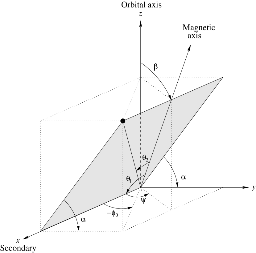
Figure 1: Orientation of the primary relative to the orbital axis and direction of the secondary centre. We also define the orientation of the magnetic field of the primary, tilted by $\beta$ from the $z$ axis and whose projection in $xy$ plane makes an angle $\psi$ with the $x$-axis. The dot represents where the field line that goes through the secondary crosses the surface of the primary, the position of the spot makes an angle $\theta_{1}-\theta_{2}$ with the $x$-axis.

Following the model presented by Wu et al. (2002) we consider a system in which one star (which we call the secondary star) orbits within the magnetic field of its companion, the primary star. An asynchronism between the spin of the primary star and the orbit induces an electric current to flow along the field lines connecting the two stars, with energy dissipated mainly where these field lines enter the surface of the primary star. In the Jupiter–Io system the observed emission lies within $6^{\circ}$ of the theoretically predicted foot point (Clarke et al., 1996). In our case we expect the emission to be even nearer to the foot point because of the smaller degree of asynchronism.

Our task is to identify the positions of these foot points, and then work out for how long they are visible for a given orbital inclination. We treat them as points in order to allow the model to match the 40% dark phase during which X-rays disappear (constraint I, section 2) as easily as possible. To allow the model flexibility in matching the bright phase, we allow for the maximum size of the spots, as described at the end of this section.

We will now describe the geometry of the model with reference to Fig. 1. We work with a right-handed Cartesian coordinate system $(x$,$y$,$z)$ centred upon the primary star, with the $x$-axis pointing towards the secondary star, the $y$-axis parallel to the direction of motion of the secondary star, and the $z$-axis along the orbital axis (Fig. 1). The axis of the magnetic dipole is tilted by an angle $\beta$ (often called the magnetic colatitude) with respect to the spin and orbital axes, which we take to be aligned. The azimuthal angle or magnetic longitude of the dipole $\psi$ is defined by the angle between its projection onto the orbital plane (the $x$-$y$-plane) and the $x$-axis. In Wu et al. (2002)’s model there is an asynchronism between the period of the binary and the spin period of the magnetic white dwarf. Therefore $\psi$ is the angle that completes a cycle every few days owing to the asynchronism between the orbital frequency $\omega_{o}$ and the spin frequency of the primary star $\omega_{s}$:

$$\psi=(\omega_{s}-\omega_{o})t+\psi_{0}.$$ (2)

Wu et al. (2002) estimate the asynchronism $(\omega_{s}-\omega_{o})/\omega_{o}$ to be 1 part in 1000. This means that all possible azimuths of the magnetic axis compared to the line of centres of the two stars are explored within $\sim 1000$ orbits, which is only a few days. If the magnetic axis is tilted with respect to the orbital axis, such azimuth variation causes the phase of the light curve maxima to vary back and forth relative to any long term trend. By applying the III condition upon the phase, we effectively assume that the X-ray observations have sampled all possible relative orientations of the magnetic axis (all values of $\psi$ have been explored) and therefore we insist that the constraints of the previous section are satisfied for all $\psi$. Ideally this would be the case, and indeed with sufficient observations one can get very close to it. We will consider how close we are to this in reality in section 4.1.

We define the positions of the foot points by where the magnetic field line which passes through the centre of the secondary star crosses the surface of the primary star. This field line lies in a plane defined by the $x$-axis and the magnetic dipole vector which makes an angle $\alpha$ with the orbital plane Fig. 1. We define the orientation of the foot points in this plane with two angles $\theta_{1}$ and $\theta_{2}$ which measure the angle between the dipole axis and $x$-axis and the angle between the dipole axis and the foot point respectively.

Using the equation for dipole field lines $r=\mathcal{C}\sin^{2}\theta$, we can deduce the following relation between $\theta_{1}$ and $\theta_{2}$

$$\sin\theta_{2}=\sqrt{\frac{r_{1}}{a}}\sin\theta_{1}.$$ (3)

while from simple geometry one can show that

$$\cos\theta_{1}=\cos\psi\sin\beta,$$ (4)

and that

$$\cos\alpha=\frac{\sin\psi\sin\beta}{\sqrt{(\sin\psi\sin\beta)^{2}+\cos^{2}\beta}}.$$ (5)

To be able to calculate the visibility of the spot from the Earth, we need the orbital phase $\phi$ and the orbital inclination angle $i$, which we define in the standard manner, i.e. $i=90^{\circ}$ for an edge-on eclipsing system, $\phi=0^{\circ}$ when the magnetic primary star is at its furthest from Earth. With all angles defined, a given spot is visible while

$$\cos(\phi-\phi_{0})>-\frac{h}{A}$$ (6)

where

$$A=\sin i\sqrt{\cos^{2}(\theta_{1}-\theta_{2})+\cos^{2}\alpha\,\sin^{2}(\theta_{1}-\theta_{2})},$$ (7)

$$h=\cos i\sin\alpha\sin(\theta_{1}-\theta_{2}),$$ (8)

and

$$\tan\phi_{0}=\frac{-\cos\alpha\,\sin(\theta_{1}-\theta_{2})}{\cos(\theta_{1}-\theta_{2})}.$$ (9)

For given values of $\beta$, $i$, $\psi$ and $r_{1}/a$, it is a straightforward matter to calculate the remaining variables, and in particular to calculate the fraction of the cycle over which the spot can be seen. Before describing these calculations, we pause to consider the issue of the size of the foot points, which is important for the second of our constraints which defines the minimum period over which the spots are visible.

The sizes of the foot points are related to the size of the secondary star. If the latter is tiny, then so too are the foot points. Wu et al. (2002) give an equation for the size of the foot points (A1 of their appendix A) from which we deduce that the maximum extent in longitude of the foot points, is of order $2r_{2}/a$ radians. This will lengthen the bright phase by a corresponding amount. The maximum extent is thus set by the maximum relative size of the secondary, which is itself set by Roche geometry. For equal mass ratios, we deduce a maximum longitude extent of about $40^{\circ}$, which could extend the bright phase by $\sim 10$% of the cycle. To be conservative, we assume a maximum lengthening of $0.2$ for all models, as outlined in constraint II of section 2.

In our model we assume that the X-rays are only emitted at one of the two foot points. Allowing both spots to contribute makes matters worse. Although the restriction that the bright phase last for more than 40% of the cycle becomes easier to satisfy, it is more difficult to fit the 40% dark interval. The phase restriction is also affected negatively: for most configurations only one spot would be visible at a given time, but when the two spots are visible there would be a change in $\psi$ leading to a phase shift.

3.1 Computations

We computed the fraction of the cycle that one of the foot points is visible as a function of magnetic colatitude $\beta$ (from 0 to $180^{\circ}$) and orbital inclination (0 to $90^{\circ}$). In order to implement our assumption that we have observed all possible values of $\psi$, we search for the maximum and minimum values of the spot visibility over a finely-spaced array of $\psi$ values from 0 to $180^{\circ}$ (symmetry allows us to avoid searching over $360^{\circ}$). In order to obey the constraints of section 2, we must have that

1. the maximum time that the spot is visible must be less than 0.6 of a cycle,

2. the minimum time that the spot is visible must be more than 0.4 of a cycle.

The masses of the white dwarfs have to be less than $1.4\,\mathrm{M}_{\odot}$ (Chandrasekhar’s limit) and larger than the Roche lobe filling mass: for RXJ0806.3+1527 $M_{1},M_{2}>0.12\,\mathrm{M}_{\odot}$ and for V407 Vul $M_{1},M_{2}>0.065\,\mathrm{M}_{\odot}$. We calculated the binary separation using Kepler’s third law and the radius of the white dwarf using Eggleton’s mass-radius relation quoted by Verbunt & Rappaport (1988).

4 Results

Figure 2: Geometrical constraints for the unipolar modal, for V407 Vul in the left hand panel and for RXJ0806.3+1527 in the right hand panel. The shaded areas represent the parameter space ruled out by the restrictions I, II, III respectively in the top, middle and bottom panels.

Figure 3: Track of the heated spot (dashed lines) viewed from above the primary star (outermost circle) for different choices of inclination of the magnetic field $\beta$. For $\beta$ smaller than the critical angle $\beta_{c}$ the track is always on the side facing the secondary (towards the right). In this case the X-ray pulse phase varies over a restricted range indicated here by the two tangential lines for $\beta=10^{\circ}$. For $\beta$ greater than $\beta_{c}$ the heated spot makes a complete circle around the polar axis of the primary star causing a complete phase shift of the X-ray pulses over one beat period.

Figure 4: The figure shows examples of X-ray phase light curves for V407 Vul. A, B and C represent different choice of parameters shown in Fig. 2 with three possible $\psi=$  $0^{\circ}$, $90^{\circ}$ and $180^{\circ}$ to illustrate the phase shift. For A, $\beta=5^{\circ}$ and $i=87^{\circ}$, for B, $\beta=5^{\circ}$ and $i=45^{\circ}$ and for C, $\beta=135^{\circ}$ and $i=87^{\circ}$. In all the figures the flux is normalised to unity.

We start by discussing how the constraints of section 2 restrict the possible values of the magnetic tilt $\beta$ and the inclination angle $i$ for typical white dwarf masses of $0.6\,\mathrm{M}_{\odot}$ (Fig. 2). The first constraint (top panels) rules out combinations of low inclination and small angle between the magnetic field and the spin axis. This is because we would be looking at the north pole and the spot would also be in the northern hemisphere, i.e. it would be visible for most of the time which would violate the maximum 60% bright phase. Note that there is a critical magnetic colatitude when $\beta_{c}=\theta_{2}$ given by

$$\tan\beta_{c}=\sqrt{r_{1}/a}$$ (10)

such that when the magnetic axis is tilted away from the secondary star ($\psi=180^{\circ}$), the foot point lands upon the spin pole of the primary star and will therefore always be visible, no matter the orbital inclination. For $M_{1}=M_{2}=0.6\,\mathrm{M}_{\odot}$, $\beta_{c}=15^{\circ}$ for V407 Vul and $19^{\circ}$ for RX J0806.3+1527. This critical value is clear in Fig. 2.

The second constraint is symmetric to the first, so that the foot point cannot lie too close to the south pole without leading to too short a visibility fraction (central panels of Fig. 2).

The third constraint, that of phase, is highly restrictive as it removes all colatitude values in the range $\beta_{c}<\beta<180-\beta_{c}$. In other words, the magnetic and orbital axes must be nearly aligned in order for the phases not to wander. The reason for this is that for $\beta$ in the excluded range, the phase switches by 180 degrees depending upon whether the magnetic dipole is oriented towards or away from the secondary star. This would show up as a large deviation in the X-ray pulses from a smooth trend. Note that our exact phase constraint ($<0.2$ of a cycle variation) is actually a little more restrictive still since significant phase wander occurs as $\beta$ nears $\beta_{c}$.

To better illustrate this, Fig. 3 shows the track of the heated spot on the primary star during one beat period as seen in the rotating frame of the binary. We can see that, for $\beta<\beta_{c}$ (or the symmetric case $\beta>180-\beta_{c}$), the phase offset is restricted to lie within the region defined by the two tangential lines to the small dashed circle but for $\beta>\beta_{c}$ the phase offset goes through a complete cycle. For the dipole field we assume, one can show that the tracks are perfect circles.

To visualise the three constraints Fig. 4 shows examples of the light curves using some combinations of parameters that illustrate the problems of this geometry. When $\beta=5^{\circ}$ and $i=87^{\circ}$ (marked ‘A’ on Fig. 2) the light curve obeys the first three constraints and it is similar to the observed data. In the second case considered $\beta=5^{\circ}$ and $i=45^{\circ}$ (‘B’ in Fig. 2) the spot is always visible and therefore fails to obey constraint I. In the third example $\beta=135^{\circ}$ and $i=87^{\circ}$ (‘C’) the phase constraint is not complied with and there is a large phase shift between $\psi=0^{\circ}$, and $\psi=180^{\circ}$.

The fourth and last constraint is the restriction that the system does not eclipse. This is independent of magnetic tilt and depends only upon the masses of the two stars for a given orbital period.

In figure 5 we show the possible values allowed by the combination of all the constraints mentioned above, for $M_{1}=M_{2}=0.6\,\mathrm{M}_{\odot}$, other white dwarf masses will be considered later. The figures also show the maximum inclination for which the system will not have eclipses (horizontal lines). Together, the constraints rule out all parameter combinations.

Figure 5: The lines going from top-left to bottom-right represent the parameter space ruled out by the combination of the constraints I, II and III. The only regions left out are two triangles in the top corners of the parameter space. However these are also ruled out when we include the absence of eclipses which rules out the regions shown by the oppositely sloped lines. Therefore we are left with no possible solution in the case of $M_{1}=0.6M_{\odot}$ and $M_{2}=0.6M_{\odot}$. Note that the vertical scale here has been adjusted to show only the top parts of Fig. 2

4.1 Detailed analysis of the phase constraint

We assumed for simplicity that we have seen all possible values of the angle $\psi$ which measures the azimuth of the magnetic dipole within the binary. However, in this section we investigate further if this is really the case or if the observations of the two systems carried out so far are not sufficient to eliminate the possibility that the systems were only observed over a small range of $\psi$, thereby increasing the available region of parameter space.

We only used the X-ray data because according to the unipolar inductor model, the optical flux is from the secondary star and is therefore locked to the orbit.

Wu et al. (2002) deduced that for V407 Vul an asynchronism of 1 part in 1000 would be enough to explain the luminosity observed.

The degree of asynchronism is a little arbitrary so we explored several values in the range 1 part in 100000 to 1 part in 700 for V407 Vul. We used the dates and durations of the X-ray observations of V407 Vul to compute the phase shifts that would have been seen for a set of degrees of asynchronism in this range. The largest asynchronism of 1 part in 700 is set by the length of the longest observation and is such that this observation covered an entire beat cycle. A degree of asynchronism larger than this returns us to our original assumption of complete coverage of $\psi$. The phase shifts were then fitted with a quadratic ephemeris and the scatter around the ephemeris was minimised by subtraction or addition of whole cycles where necessary. This process simulates the treatment of the observed pulse times by, for example, Strohmayer (2004), and acts to reduce the phase shifts somewhat. Finally the values were minimised over the (unknown) phase offset $\psi_{0}$ by repetition of the computation for 40 values equally spaced around a cycle and retention of the minimum shift calculated. This is in the spirit of trying to give the unipolar inductor model the benefit of the doubt where possible.

We applied the same method to RX J0806.3+1527. In this case the observations were much shorter and so our range of the degree of asynchronism is 1 part in 100000 to 1 part in 80 which corresponds to the period of the longest observation which was made with XMM-Newton. We reduced archival XMM-Newton data from November 2002 to complement the phase timing by Strohmayer (2003). Using the latest published value for the period $P$ and its derivative $\dot{P}$ (Hakala et al., 2004) and the phase 0 of the phase folded X-ray light curve of Israel et al. (2003) $\mathrm{MJD}=52225.36153\pm 0.00004$ for comparison, we obtained a phase shift for Nov 2002 close to zero, so we include the times for these observations in our study. However, given present uncertainties in both $P$ and $\dot{P}$, we cannot rule out a larger phase shift between any of the observations.

Our results are shown in Fig. 6 in which we plot the phase shift, minimised over $\psi_{0}$, as a function of the degree of asynchronism that would have been seen in the past observations of V407 Vul and RX J0806.3+1527, for different inclinations of the magnetic field $\beta$ if the Wu et al. (2002) model is correct. (Note that the phase shift is independent of the orbital inclination $i$.)

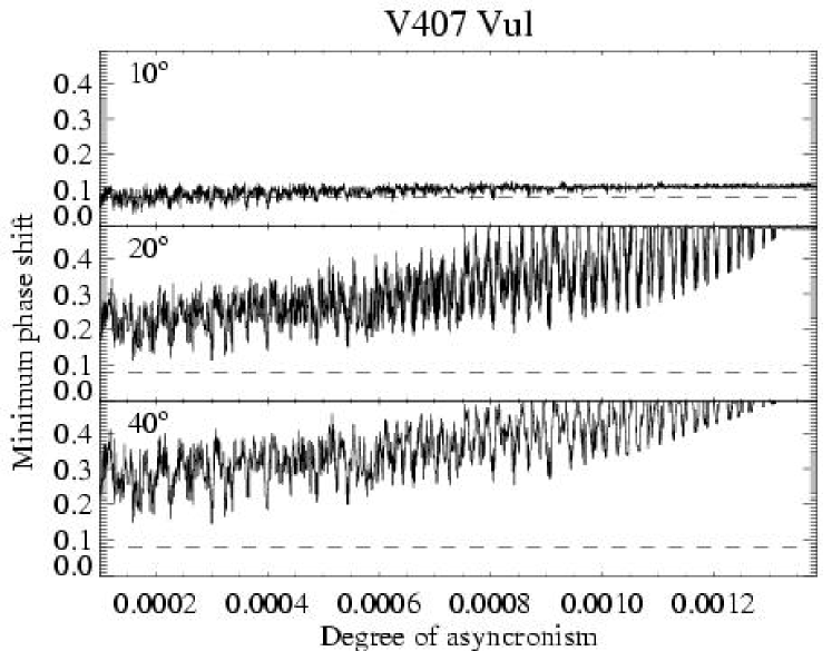
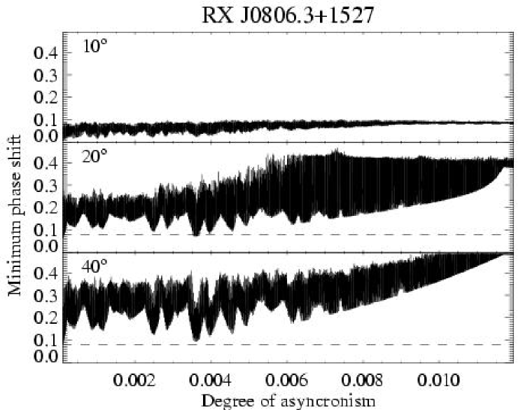
Figure 6: The minimum phase shift relative to a quadratic ephemeris as a function of the degree of spin/orbit asynchronism for $\beta=10^{\circ}$, $20^{\circ}$ and $40^{\circ}$. The dashed line represents the maximum phase shift measured in the observations of the two stars $=0.08$.

As expected from our simple phase constraint, small angles of $\beta$ such that $\beta<\beta_{c}$ do have low enough phase shifts to match the observations which show at most a deviation of $0.08$ cycles for both systems. For V407 Vul, when $\beta>\beta_{c}$, even the minimised values that we plot are consistently larger than is observed, although the phase shifts do not match the value of $0.5$ that we would predict for perfect observational coverage. In other words, the observations of V407 Vul are extensive enough that our conclusion that the region $\beta_{c}<\beta<180-\beta_{c}$ is ruled out by the absence of phase shifts remains unchanged.

The much sparser observations of RX J0806.3+1527 on the other hand, do not allow us to rule out large $\beta$ angles with confidence as some frequencies show relatively small phase shifts. Clearly more observations of RX J0806.3+1527 are required. Having said this, if the unipolar inductor model were to be let off the hook by this means, it would be at a significant price because then the X-ray phases measured so far would not necessarily be a true reflection of the orbital phase and the present indications of spin-up Hakala et al. (2004), which depend in large part upon ROSAT data, could well be spurious.

5 Discussion

In this section we will discuss the limitations of our analysis, the effect of varying the white dwarf masses and the effect of the spot size upon the allowed parameter space.

5.1 Effects of different masses

All of the constraints depend upon the masses of the white dwarfs, so in this section we explore whether changing the mass can allow some models to work. Increasing the size of the primary star helps by shifting the foot points toward its equator. Therefore, we expect an easing of the problem for small primary star masses, except that this will make the eclipse restriction harder to satisfy. Increasing the mass of the secondary star on the other hand is entirely beneficial since it increases the maximum inclination angle for which there is still no eclipse. However, it has to be said that there is some inconsistency here with respect to the foot point size which will be nowhere near our assumed maximum. If this could be taken into account reliably, it would count against large masses for the secondary star, but we do not attempt to allow for this subtlety here.

For V407 Vul we find that a very small area of the $\beta$–$i$ parameter space is allowed for $M_{1}=1.4\,\mathrm{M}_{\odot}$ and $M_{2}>1.3\,\mathrm{M}_{\odot}$, or for $M_{1}=M_{2}=1.3\,\mathrm{M}_{\odot}$. The parameter space allowed requires the magnetic and spin axes to be nearly aligned ($\beta<2^{\circ}$ or $\beta>178^{\circ}$), the system to have a very specific orbital inclination ($88.2<i<88.8^{\circ}$) and masses right at the top of the range for white dwarfs. Together the combination is very unlikely, and we will see below that it causes other problems. The case of RX J0806.3+1527 is still tougher, and there are only possible solutions for $M_{1}=1.4\,\mathrm{M}_{\odot}$ and $M_{2}=1.4\,\mathrm{M}_{\odot}$ which are even more restrictive for both $\beta$ and $i$ ($\beta<1.5^{\circ}$ or $\beta>178.5^{\circ}$ and $87.8<i<88.3^{\circ}$ )

There are no known white dwarfs with masses as high as required here. Moreover, even if the masses really were this high, they would be in severe conflict with one of the main pieces of evidence in favour of the unipolar model, which are the measurements of decreasing period, presumed to be caused by gravitational radiation. We computed the values of the spin up of the systems for the lowest masses that have any available parameter space assuming a detached binary driven only by gravitational radiation loss. For the case of V407 Vul with $M_{1}=M_{2}=1.3\,\mathrm{M}_{\odot}$ the spin up rate would be $\sim 3.6\times 10^{-16}\,\mathrm{Hz}\,\mathrm{sec}^{-1}$, some fifty times the measured value reported by Strohmayer (2004) of $7.0\pm 0.8\times 10^{-18}\,\mathrm{Hz}\,\mathrm{sec}^{-1}$, while in the case of RX J0806.3+1527 for $M_{1}=M_{2}=1.4\,\mathrm{M}_{\odot}$ the spin up rate would be $\sim 2.3\times 10^{-15}\,\mathrm{Hz}\,\mathrm{sec}^{-1}$, five times the measured value reported by Strohmayer (2003) and Hakala et al. (2004) of $6.00\pm 0.1\times 10^{-16}\,\mathrm{Hz}\,\mathrm{sec}^{-1}$. In consequence even the tiny region of parameter space that is opened up at high mass fails to match up against what we know of these systems.

5.2 Spot Size

We assumed a maximum spot size that would extend the visibility of a point spot for 0.2 of a cycle which corresponds to the secondary star filling its Roche lobe , i.e. a very low mass secondary. But as seen in our analysis the problems facing the unipolar modal are eased at high masses. As the spot size depends greatly on the secondary mass, the actual size of the footprints for the masses considered before would be only 0.02 of a cycle for $M_{1}=0.6\,\mathrm{M}_{\odot}$ and 0.003 for $M_{1}=1.4\,\mathrm{M}_{\odot}$ in the case of V407 Vul. With such a small spot size it would be impossible to accommodate the model because for example if we force the bright phase to be more than 0.5 of a cycle, we eliminate all the values that were allowed by constraint I i.e. the first two constraints alone would rule out the model.

There are some effects that might help make the spot larger, for example the X-rays could perhaps come from a vertical extended region (along the field lines), that would allow us to see them for a little bit longer, although this might be difficult to reconcile with the thermal nature of the X-ray spectrum. Perhaps the foot points can leave a trail along the azimuthal direction ($\phi_{0}$), that would enlarge the size of the emitting region. The theoretical estimates of the cooling time scale indicate that trailing is unlikely to be significant (Stockman et al., 1994), but we can in any case show that increasing the visibility duration has only a limited effect in helping the unipolar model. In Fig. 7 we show the effect of increasing the spot size upon the available parameter space. Only for very large spot sizes, covering $>0.3$ of a cycle in azimuth, is possible parameter space opened up. (Note that $0.6$ is the largest possible azimuth extent given the need for a $40\%$ off period.)

In summary, even a fairly radical alteration to allow much larger spots than are predicted by the unipolar model at best opens up a small region of parameter space with $\beta>173^{\circ}$, $74^{\circ}<i<81^{\circ}$. It is clearly unlikely that these applies to two independent systems.

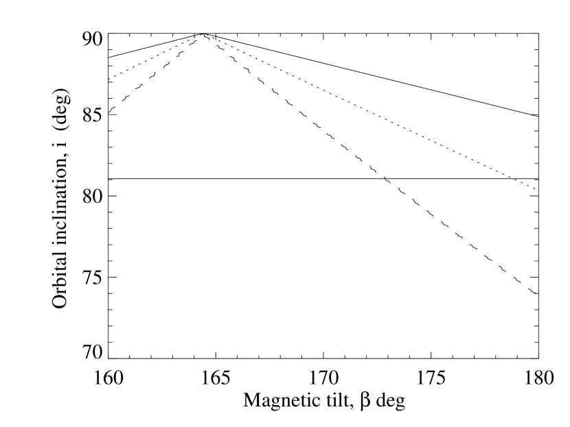
Figure 7: The top-left region of the parameter space where we show the constraint II for several maximum spot sizes 0.2 of a cycle (solid line), 0.3 of a cycle (dotted line) 0.6 of a cycle (dashed line) for white dwarf masses of $0.6\,\mathrm{M}_{\odot}$ for 407 Vul. The allowed region is always above the line. So for the maximum spot size larger then 0.3 of a cycle there is a small allowed region in parameter space (triangle covering $\beta>173^{\circ}$ $74^{\circ}<i<81^{\circ})$.

6 Conclusion

Assuming a dipolar field geometry and that the spin and orbital axis are aligned, we find that the unipolar inductor model presented by Wu et al. (2002) cannot match the X-ray light-curves of the two systems V407 Vul and RX J0806.3+1527. It fails because the foot points which produce the X-rays are situated quite close to the magnetic poles, while at the same time the magnetic axes are forced to lie almost parallel to the spin axes of the primary stars to avoid excessive phase shifts in the X-ray pulses. This then means that to obtain the near 50:50 on/off light curves observed, both systems have to be seen at such high orbital inclination ($>88^{\circ}$) that they would eclipse, and yet no eclipses are seen. High masses for the component stars permit tiny regions of viable orbital inclination/magnetic inclination parameter space, but lead to very large gravitational wave losses inconsistent with observed period changes. If for some reason the heated spots are much larger than the unipolar model predicts a small region of parameter space is allowed, but even this requires fine tuning for two systems. The only remaining chinks of light for the unipolar inductor model is that RX J0806.3+1527, owing to relatively sparse X-ray coverage, could have a relatively highly inclined dipole without our having spotted the large phase shifts so far, or possibly the field configurations are very different from a dipole in the two stars. Further observations are encouraged to close this loophole. We have been careful where possible to err in favour of the unipolar inductor model; we still have to conclude that it is not viable in its current form.

7 Acknowledgements

SCC Barros is supported by Fundação para a Ciência e Tecnologia e Fundo Social Europeu no âmbito do III Quadro Comunitário de Apoio. TRM acknowledges the support of a PPARC Senior Research Fellowship. GN is supported by NWO-VENI grant 639.041.405. DS acknowledges support of a Smithsonian Astrophysical Observatory Clay Fellowship.

References

- Clarke et al. (1996) Clarke J. T., Ballester G. E., Trauger J., Evans R., Connerney J. E. P., Stapelfeldt K., Crisp D., et al., 1996, Science, 274, 404
- Cropper et al. (1998) Cropper M., Harrop-Allin M. K., Mason K. O., Mittaz J. P. D., Potter S. B., Ramsay G., 1998, MNRAS, 293, L57
- Hakala et al. (2004) Hakala P., Ramsay G., Byckling K., 2004, MNRAS, 353, 453
- Hakala et al. (2003) Hakala P., Ramsay G., Wu K., Hjalmarsdotter L., Järvinen S., Järvinen A., Cropper M., 2003, MNRAS, 343, L10
- Israel et al. (2003) Israel G. L., Covino S., Stella L., Mauche C. W., Campana S., Marconi G., Hummel W., Mereghetti S., Munari U., Negueruela I., 2003, ApJ, 598, 492
- Israel et al. (2002) Israel G. L., Hummel W., Covino S., Campana S., Appenzeller I., Gässler W., Mantel K.-H., et al., 2002, A&A, 386, L13
- Israel et al. (1999) Israel G. L., Panzera M. R., Campana S., Lazzati D., Covino S., Tagliaferri G., Stella L., 1999, A&A, 349, L1
- Marsh & Steeghs (2002) Marsh T. R., Steeghs D., 2002, MNRAS, 331, L7
- Motch et al. (1996) Motch C., Haberl F., Guillout P., Pakull M., Reinsch K., Krautter J., 1996, A&A, 307, 459
- Nelemans et al. (2001) Nelemans G., Portegies Zwart S. F., Verbunt F., Yungelson L. R., 2001, A&A, 368, 939
- Norton et al. (2004) Norton A. J., Haswell C. A., Wynn G. A., 2004, A&A, 419, 1025
- Ramsay et al. (2000) Ramsay G., Cropper M., Wu K., Mason K. O., Hakala P., 2000, MNRAS, 311, 75
- Ramsay et al. (2002) Ramsay G., Hakala P., Cropper M., 2002, MNRAS, 332, L7
- Ramsay et al. (2002) Ramsay G., Wu K., Cropper M., Schmidt G., Sekiguchi K., Iwamuro F., Maihara T., 2002, MNRAS, 333, 575
- Stockman et al. (1994) Stockman H. S., Schmidt G. D., Liebert J., Holberg J. B., 1994, ApJ, 430, 323
- Strohmayer (2002) Strohmayer T. E., 2002, ApJ, 581, 577
- Strohmayer (2003) Strohmayer T. E., 2003, ApJ, 593, L39
- Strohmayer (2004) Strohmayer T. E., 2004, ApJ, 610, 416
- Verbunt & Rappaport (1988) Verbunt F., Rappaport S., 1988, ApJ, 332, 193
- Wu et al. (2002) Wu K., Cropper M., Ramsay G., Sekiguchi K., 2002, MNRAS, 331, 221