B-type Supergiants in the SMC: Chemical compositions and comparison of static and unified models

High-resolution UCLES/AAT spectra are presented for nine B-type supergiants in the SMC, chosen on the basis that they may show varying amounts of nuclear-synthetically processed material mixed to their surface. These spectra have been analysed using a new grid of approximately 12 000 non-LTE line blanketed tlusty model atmospheres to estimate atmospheric parameters and chemical composition. The abundance estimates for O, Mg and Si are in excellent agreement with those deduced from other studies, whilst the low estimate for C may reflect the use of the C ii doublet at 4267Å. The N estimates are approximately an order of magnitude greater than those found in unevolved B-type stars or H ii regions but are consistent with the other estimates in AB-type supergiants. These results have been combined with results from a unified model atmosphere analysis of UVES/VLT spectra of B-type supergiants (Trundle et al. Tru04 (2004)) to discuss the evolutionary status of these objects. For two stars that are in common with those discussed by Trundle et al., we have undertaken a careful comparison in order to try to understand the relative importance of the different uncertainties present in such analyses, including observational errors and the use of static or unified models. We find that even for these relatively luminous supergiants, tlusty models yield atmospheric parameters and chemical compositions similar to those deduced from the unified code fastwind.

1 Introduction

The spectra of early-type supergiants provide an excellent method for studying Local Group galaxies due to their high intrinsic luminosities (typically 1 000 to 10 000 L_⊙). Yet it is this extreme luminosity which also gives rise to the complex nature of supergiants, whose stellar wind and extended atmospheres drive them away from a plane-parallel, Local Thermodynamic Equilibrium (LTE) regime. Developments in theoretical techniques that incorporate non-LTE effects, line blanketing, sphericity and mass-loss have lead to a resurgance of interest in these objects (for example see Hubeny Hub88 (1988); Hubeny et al. Hub98 (1998); Santolaya-Rey et al San97 (1997); Hillier & Miller Hil98 (1998)). Recent studies of OB-type Supergiants in the Local Group have had a number of aims including understanding the evolution of massive stars, studying the chemical composition of the host galaxy and calibrating the wind momentum versus luminosity relation for distance determinations. These studies include those of Lennon et al. (Len91 (1997)), Gies & Lambert (Gie92 (1992)), Kudritzki et al. (Kud99 (1999)), McErlean et al. (McE99 (1999)) and Repolust et al. (Rep04 (2004)) in our Galaxy, Fitzpatrick & Bohannan (Fit93 (1993)), Puls et al. (Pul96 (1996)), Dufton et al. (Duf00 (2000)), Korn et al. (Kor02 (2002)), Trundle et al. (Tru04 (2004, 2005)) and Venn (Ven99 (1999)) for the Magellanic System, Venn et al. (Ven00 (2000)), Smartt et al. (Sma01 (2001)) and Trundle et al. (Tru02 (2002)) for M31, Monteverde et al. (Mon97 (1997, 2000)) and Urbaneja et al. (Urb02 (2003)) for M33 and Kaufer et al. (Kau04 (2004)), Urbaneja et al. (Urb03 (2003)) and Venn et al. (Ven01 (2000); 2003b ) for other Local Group galaxies. Studies of the progenitor O-type stars (see Bouret et al. Bou03 (2003), Hillier et al. Hil03 (2003), Heap et al. Hea04 (2004)) and B-type giants (see Korn et al. Kor02 (2002), Lennon et al. Len03 (2003)) have also provided relevant observations to aid our understanding of the evolution of the surface chemical composition of early-type stars.

Since the studies of Jaschek & Jaschek (Jas67 (1967)), Walborn (Wal72 (1972)) and Dufton (Duf72 (1972)), the dispersion of observed nitrogen abundances in OBA-type stars selected within a particular metallicity environment has stimulated continuing interest in the area of massive stars. These changes in the surface chemical composition of hot stars are closely coupled to their rotational velocities. Current theoretical models require initially high rotational velocities in order to mix nucleosynthetically processed material to the surface (Heger & Langer Heg00 (2000); Maeder & Meynet Mae00 (2000, 2001)). In turn these models predict that B-type supergiants and giants should still be rotating relatively rapidly with larger rotational velocities in lower metallicity regions where the loss of angular momentum through the strong stellar wind is less significant. However as discussed by Howarth et al. (How94 (1994)), Lennon et al. (Len03 (2003)) and Trundle et al. (Tru04 (2004)), this appears inconsistent with the observed widths of the metal line spectra. Ryans et al. (Rya02 (2002)) have attempted to distinguish between the different broadening mechanisms (viz. microturbulence, rotation and macroturbulence). For a sample of Galactic supergiants, they found that the contribution of rotation to the line-broadening was relatively small, in turn leading to large discrepancies with the theoretical predictions.

In this paper, we present high resolution observations of a sample of SMC supergiants chosen from a preliminary exploration of B-type supergiants by Dufton et al. (Duf00 (2000)). The selection of targets was made on the basis that they might show different degrees of nucleosynthetic processed material at their surface. These have been analysed using a new grid of approximately 12 000 models computed with the non-LTE codes tlusty and synspec (Hubeny Hub88 (1988); Hubeny & Lanz Hub95 (1995); Hubeny et al. Hub98 (1998)). These models do not include any contribution from a stellar wind and therefore, for two targets, we have compared our results with those deduced by Trundle et al. (2004) from the unified code fastwind (Santolaya-Rey et al. San97 (1997); with some updates described in Herrero et al. Her02 (2002) and Repolust et al. Rep04 (2004)) to investigate the magnitude of both observational and theoretical uncertainties. In a companion paper, we intend to obtain reliable estimates of the actual projected rotational velocities of our own and other SMC targets using the methods discussed by Ryans et al. (Rya02 (2002)). These should allow a better understanding of the relationship between the chemical evolution and rotation for massive stars.

Table 1: Observational summary of the nine program stars. Spectral types are those assigned by Lennon (1997). Apparent V-magnitudes are taken from Massey (2002) where available and supplemented by Garmany et al. (1987;^†)

Star	V	Spec.	S/N ratio	$v_{\mathrm{r}}$	FWHM
	[mag]	Type		km s-1
AV 78	11.05	B1.5Ia+	130	178	80
AV 215	12.69	BN0Ia	90	159	115
AV 242	12.11†	B1Ia	110	142	100
AV 303	12.78	B1.5Iab	100	186	65
AV 374	13.09	B2Ib	65	125	70
AV 462	12.54	B1.5Ia	115	126	70
AV 472	12.62	B2Ia	90	138	70
AV 487	12.58	BC0Ia	125	183	100
SK 191	11.86†	B1.5Ia	125	134	130

2 Observations and data reduction

The high-resolution, spectroscopic data presented here were obtained during an observing run with the 3.9-m Anglo-Australian Telescope (AAT) from 29 September to 1st October 1998 inclusively. The University College of London Échelle Spectrograph (UCLES) was used with the 31 lines mm^-1 grating and with a TeK 1K$\times$1K CCD, providing complete spectral coverage between $\lambda\lambda$3900–4900 Å at a FWHM resolution of $\sim$0.1 Å. Conditions were excellent throughout the three night run, with stellar exposures being bracketed with Cu-Ar arc exposures for wavelength calibration. Observations were obtained for nine supergiants and these are summarized in Table 1. Listed are the stellar V-magnitude (taken from Garmany et al. Gar87 (1987) and Massey Mas02 (2002)), spectral types (from Lennon Len97 (1997)), the signal-to-noise (S/N) ratio at approximately 4500Å, the heliocentric radial velocity ($v_{\mathrm{r}}$) and the typical full-width-half-maxima (FWHM) of the metal absorption line spectrum. The latter two quantities were estimated as discussed below, whilst the S/N ratios were deduced by fitting low order polynomials to the continuum. Care was taken to include continuum regions from different parts of the blaze profile and hence these estimates should be considered as conservative, particularly given the significant wavelength overlap between adjacent orders.

The choice of targets was based on the spectral types deduced by Lennon (Len97 (1997)) and the preliminary non-LTE analysis of Dufton et al. (Duf00 (2000)) of intermediate dispersion spectroscopy. In particular, we attemped to sample a range of luminosity types (ranging from Ia⁺  to Ib) and with varying degrees of mixing of nucleosynthetic material to the surface. For the latter, we included both BN and BC spectral types and stars with different ratios of N ii to C ii equivalent widths (see Fig. 9 of Dufton et al.).

The two dimensional CCD datasets were reduced using standard procedures within IRAF (Tody Tod86 (1986)). Preliminary processing of the CCD frames such as over-scan correction, trimming of the data section and flat-fielding were performed using the CCDRED package (Massey Mas97 (1997)), whilst cosmic-ray removal, extraction of the stellar spectra, sky-subtraction and wavelength calibration were carried out using the SPECRED (Massey et al. Mas92 (1992)) and DOECSLIT (Willmarth & Barnes Wil94 (1994)) packages.

Equivalent widths (EWs) of lines were measured using the STARLINK spectrum analysis program DIPSO (Howarth et al. How94 (1994)). Low order polynomials were fitted to the adjacent continuum regions for normalisation and Gaussian profiles to the metal and non-diffuse helium lines using non-linear least square routines. As discussed by Ryans et al. (Rya03 (2003)), the profiles of metal absorption lines in the spectra of early-type supergiants are well represented by a Gaussian profiles. Tests using a different profile shape showed that this assumption was not critical to the fitting procedure.

In addition the central wavelength and widths of the metal lines could be used to determine the stellar radial velocity and FWHM, which are summarized in Table 1. Typically 10 relatively strong, isolated lines were used for the former, whilst the FWHM were estimated from the Si iii multiplet near 4560Å, which was well observed in all our spectra. Standard deviations were typically $\pm$2 km s^-1and $\pm$5 km s^-1respectively, with the values for the FWHM being rounded to the nearest 5 km s^-1. For the hydrogen lines, the identification of the continuum was complicated by the presence of a significant echelle ripple. In these cases the continua of the adjacent orders were moved to a common wavelength scale, fitted using low order polynomials and merged. This merged spectrum, which should represent the echelle ripple for the order containing the hydrogen line was then used to rectify the relevant order prior to normalisation. Profiles were then extracted with the continuum levels being defined at $\pm$16 Å from the line centre.

3 Spectral analysis

3.1 Model atmosphere calculations

The analysis is based on grids of non-LTE model atmospheres calculated using the codes tlusty and synspec (Hubeny Hub88 (1988); Hubeny & Lanz Hub95 (1995); Hubeny et al. Hub98 (1998)). Normally when using such codes to analyse an observational dataset, the approach is to undertake specific calculations, often in the form of grids covering a restricted range of atmospheric parameters. Such an approach has the advantage that the calculations are tailored to the specific problem. Additionally, non-LTE codes often exhibit stability problems, and these are particularly severe when trace ionic species (e.g. Si ii at higher effective temperatures or Si iv at lower effective temperature) are included. By limiting the range of atmospheric parameters considered, and by selecting the model ions to be included, these stability problems can be ameliorated. However this approach is inefficient when attempting to analyse either large observational datasets or different datasets for similar types of objects.

We are therefore developing an approach based on the calculation of large grids covering the range of atmospheric parameters appropriate to B-type stars. One fundamental assumption is that the metal line blanketing is dominated by Fe and we return to its validity later in this section. Then the structure of the atmosphere is defined by the Fe abundance (or ‘metallicity’), the effective temperature ($T_{\mathrm{eff}}$), gravity ($g$) and microturbulence ($\xi_{\mathrm{t}}$, which affects the amount of blanketing). Currently we are calculating 4 grids with metallicities appropriate to our Galaxy (i.e. $[\frac{Fe}{H}]$ = 7.5 dex), the LMC (metallicity reduced by 0.3 dex), SMC (metallicity reduced by 0.6 dex), and low metallicity regimes (metallicity reduced by 1.1 dex). Due to limitations on the available CPU power we adoped the ‘classical’ tlusty ODF Fe model ions for these calculations. The models ions for the light elements that have been explicitly included in the non-LTE calculations, together with their origins and from where they may be obtained, are summarized in Table 2. These models come from two main sources, which are discussed in, eg. Allende Prieto et al. (All03 (2003)) and Lanz and Hubeny (Lan03 (2003)).

Table 2: Source of model ions used in generating the non-LTE model atmosphere grids. These model ions are discussed in Lanz and Hubeny (Lan03 (2003); designated tlusty) and Allende Prieto et al. (All03 (2003); designated Allende). They are available from http://tlusty.gsfc.nasa.gov/ and http://hebe.as.utexas.edu/ respectively.

Ion	Levels	Source
H i	16	tlusty
He i	24	tlusty
He ii	14	tlusty
C ii	39	tlusty
C iii	23	tlusty
N ii	51	Allende
N iii	32	tlusty
O ii	74	Allende
O iii	29	tlusty
Mg ii	31	Allende
Si ii	46	Allende
Si iii	74	Allende
Si iv	23	tlusty
S ii	14	tlusty
S iii	20	tlusty
Fe ii	35	tlusty
Fe iii	50	tlusty
Fe iv	43	tlusty

For each metallicity (i.e. Fe abundance), we consider approximately 120 different $T_{\mathrm{eff}}$-log g points (see Fig. 1), which are appropriate to B-type stars ranging from the main-sequence to the Eddington limit. At each $T_{\mathrm{eff}}$–log g point, we then calculate 25 models covering 5 values of $\xi_{\mathrm{t}}$  and 5 sets of light metal abundances, which are appropriate to the underlying metallicity regime. This corresponds to approximately 3 000 models per metallicity or 12 000 models in total.

The analysis of a spectrum is then relatively straightforward and fast. One selects an appropriate metallicity grid, and then analyses spectral features to determine first the atmospheric parameters and then the stellar chemical composition. The process is currently semi-automated, and will be further automated in the light of experience gained regarding those areas which will continue to require user intervention. Further information (on for example the spectral lines incorporated in synthesis calculations and the light element abundances adopted in different grids) is available at http://star.pst.qub.ac.uk/.

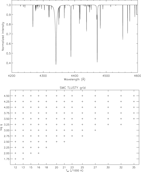
Figure 1: The bottom panel indicates the range of effective temperatures ($T_{\mathrm{eff}}$) and gravities (log g) covered by our proposed grids, with the lowest gravity models being close to the Eddington limit. At each point, 100 models are calculated covering a range of microturbulence, metallicity and light metal abundances. In total, this leads to approximately 12 000 models. The top panel shows the predicted spectrum for a small wavelength region from a typical model with an effective temperature of 20 000K, logarthmic gravity of 3.0 dex, microturbulence of 10 km s^-1and default light element abundances for the SMC.

The major difficulty with the approach outlined above is to maintain stability over the wide range of atmospheric parameters (illustrated in Fig. 1), which in turn leads to different ionic species and indeed atomic processes being important in different parts of the grid. Closely associated with this has been the problem of quality control for the very large number of proposed models. However we have now completed the SMC metallicity grid and have tested this against existing calculations using tlusty and detail/surface (see Becker & Butler Bec88 (1988, 1989, 1990); Butler But84 (1984); Giddings Gid81 (1981); Korn et al. Kor02 (2002); McErlean et al. McE99 (1999) for details of atomic data and codes). Both the overall agreement and expected differences (due e.g. to improved model ions) are highly encouraging. Difficulties remain for a small number of spectral features (see http://star.pst.qub.ac.uk/ for details), but these are relatively minor and should not affect the usefulness of the grids.

These models have been used to calculate spectra (see Fig. 1), which in turn provide theoretical hydrogen and helium line profiles and equivalent widths for light metals for a range of abundances. Note that as we keep the iron abundance fixed within any given grid, we have less extensive data for this element. Tests showed that the grid spacings for our atmospheric parameters was sufficiently fine to allow reliable interpolation of the theoretical hydrogen and helium profiles at intermediate values. For the theoretical metal line equivalent widths, these can then be accessed via a GUI interface written in IDL, which allows the user to interpolate in order to calculate equivalent widths and/or abundance estimates for approximately 200 metal lines for any given set of atmospheric parameters. Ryans et al. (Rya03 (2003)) reported that the increment of 0.4 dex used in our grids was fine enough to ensure that no significant errors were introduced by the interpolation procedures. Full theoretical spectra are also available for any given model. In summary these grids allow a user-friendly non-LTE analysis of hydrogen and helium line profiles and of the profiles and equivalent width of the lines of light elements over a range of iron line blanketing and atmospheric parameters appropriate to B-type stars in our Galaxy and in Local Group galaxies such as the Magellanic Clouds.

This approach is based on several assumptions. Firstly there are those implicit in the use of the tlusty/synspec package. Particularly relevant to the current analysis are the assumptions of a static atmosphere (which precludes the inclusion of a wind) and of a plane parallel geometry. We will return to these assumptions when comparing the results with those generated using the unified code fastwind (Santolaya-Rey et al. San97 (1997); Herrero et al. Her02 (2002)). Secondly although we have included line blanketing due to Fe, we have excluded that due to other iron peak elements, due to limits on the available computational power. However experience has shown that the bulk of the opacity in the regime of interest is due to Fe (Hubeny et al. Hub98 (1998)) so this simplification is unlikely to be a source of significant error. Thirdly we have also implicitly assumed that the atmospheric structure is not affected by the adopted light element (such as CNO, Mg, Si) abundances, which are constrained to vary in step. To test this assumption we have considered representative atmospheric parameters spanning our ranges of effective temperature, gravity, microturbulence and iron abundance. For each set of atmospheric parameters, we have then fixed, for example, the O abundance but recalculated models allowing the other light element abundances to vary. If the assumption that the atmospheric structure does not depend on the light element abundances is correct, the oxygen spectrum should not vary significantly within these calculations. Our tests show that, excluding very weak lines, variations in equivalent width are typically less than 1% and are always less than 5%. Additionally we have checked that our temperature structures for given sets of atmospheric parameters (and iron abundance) do not depend significantly on the light element abundances. This is illustrated in Fig. 2, where it can be seen that the temperature structures agree to typically $\pm$50K with the maximum differences being less than $\pm$150K. Hence we believe that the assumption that the atmospheric structure depends to first order on the atmospheric parameters and iron abundance is acceptable.

Figure 2: Differences in the temperature scales as a function of the Rosseland mean optical depth for models with an effective temperature of 20 000 K, logarithmic gravity of 2.5 dex, microturbulence of 10 km s^-1  and an Fe abundance appropriate to the SMC. There are five different models with baseline SMC element abundances and with light element abundances increased and decreased by 0.4 and 0.8 dex. The four plots show the difference in the temperature structure of the latter compared with that of the baseline abundance model. The small differences imply that the temperature structures are effectively independent of the light element abundances adopted.

Table 3: Atmospheric parameters and abundances of program stars. Also listed are results for the main sequence SMC target, AV 304. The number of lines considered is shown in brackets.

	AV 78	AV 215	AV 242	AV 303	AV 374	AV 462	AV 472	AV 487	SK 191	AV 304
$T_{\mathrm{eff}}$	21250	26500	21500	18000	18500	19000	19000	27000	20500	27000
log $g$	2.45	3.00	2.50	2.30	2.50	2.40	2.40	2.95	2.45	3.9
$\xi_{\mathrm{t}}$	13	13	13	14	14	16	15	11	16	3
C	6.91 (1)	–	7.06 (1)	7.15 (3)	7.07 (1)	7.00 (3)	7.06 (3)	7.24 (1)	7.00 (1)	7.36 (3)
$\sigma$	–	–	–	0.09	–	0.07	0.12	–	–	–
N	7.80 (9)	7.60 (3)	7.09 (3)	7.28 (6)	7.18 (5)	7.42 (8)	7.51 (9)	$<$7.3	7.53 (4)	6.55 (1)
$\sigma$	0.06	0.06	0.07	0.05	0.05	0.05	0.03	–	0.02	–
O	7.74 (12)	8.00 (11)	8.11 (19)	8.34 (22)	8.26 (12)	8.12 (17)	8.05 (18)	8.09 (10)	8.11 (13)	8.13 (42)
$\sigma$	0.08	0.08	0.04	0.03	0.03	0.05	0.03	0.04	0.06	–
Mg	6.79 (1)	6.67 (1)	6.60 (1)	6.69 (1)	6.62 (1)	6.73 (1)	6.67 (1)	6.79 (1)	6.71 (1)	6.77 (1)
Si	6.90 (4)	6.87 (4)	6.65 (4)	7.01 (4)	7.01 (4)	6.85 (6)	6.81 (3)	6.93 (3)	6.64 (3)	6.75 (6)
$\sigma$	0.01	0.02	0.01	0.03	0.02	0.01	0.01	0.03	0.01	–

3.2 Estimation of atmospheric parameters

The atmospheric parameters of our targets were estimated using standard techniques, viz. the silicon ionization equilibrium for effective temperaure, the profiles of the Balmer lines for gravity and the relative strength of absorption lines of an ionic species for microturbulence. These techniques have been described by, for example, Kilian (Kil92 (1992)), McErlean et al. (McE99 (1999)), Korn et al. (Kor02 (2002)) and Trundle et al. (Tru04 (2004)) and will only be briefly discussed here. However it should be noted that the estimation of the atmospheric parameters is an iterative process as they are inter-related. Additionally all the results presented below are based on the grid with an iron abundance appropriate to the SMC (i.e. 0.6 dex less than solar - Anders & Grevesse And89 (1989)). Tests were undertaken using other grids and these are discussed below.

3.2.1 Effective temperature, $T_{\mathrm{eff}}$

Initial estimates of the surface gravity were based on the calibration of McErlean et al. (McE99 (1999)). These were then used to estimate the effective temperature normally using the Si iii to Si iv ionization equilbrium. For AV 374, an additional estimate was available from the Si ii to Si iii ionization equilbrium, with the two values agreeing to within 200 K. The Si iii multiplet at approximately 4560Å  contains lines with a range of equivalent widths and hence the microturbulence could be simultaneously constrained (see Sect. 3.2.3). The final effective temperature estimates are summarized in Table 3, rounded to the nearest 500 K. The quality of the observational data implies that these will have an uncertainty of typically $\pm$1 000-2 000 K (see Sect. 4), while the assumptions implicit to tlusty will contribute additional uncertainties. We note that Lee et al. (Lee04 (2004)) have found that using grids with different Fe abundances changed the estimates by typically 500K or less and hence should not be a major source of error.

Figure 3: Observed and theoretical Balmer line proflies for AV 472. The theoretical profiles have been convolved with a Gaussian profile using the FWHM listed in Table 1. Note the filling in of the Balmer line cores due to wind emission and that this is more significant in the lower series members.

3.2.2 Surface gravity, $g$

The surface gravity was deduced by fitting theoretical profiles to the Balmer series features, H$\beta$ to H$\epsilon$. As expected the lower series members (and in particular H$\beta$) showed evidence of their profiles being affected by a stellar wind and in these cases more weight was given to the higher series members. The quality of the fit is shown in Fig. 3 for the target AV 472, where the theoretical profiles have been convolved with a Gaussian profile to allow for rotational and macroturbulent broadening. Use of grids with different Fe abundances did not affect the gravity determinations, with the major source of error (of the order of $\pm$0.2 dex) arising from observational and fitting uncertainties. The final adopted gravities, $g$ (in units of cm s^-2) are listed in Table 3).

3.2.3 Microturbulence, $\xi_{\mathrm{t}}$

The microturbulent velocity was initially determined from the Si iii multiplet at approximately 4560Å, by minimising the spread of abundances deduced from its 3 members. Subsequently the same procedure was undertaken using the rich O ii spectra in our targets. As has been found previously (see, for example, McErlean et al. McE99 (1999), Vrancken et al. Vra00 (2000) and Trundle et al. Tru04 (2004)), the O ii spectra gave estimates which were systematically larger by between 5 and 10 km s^-1. Typically 10-20 O ii lines are included but the analysis is complicated by them arising from different multiplets. Uncertainties in the atomic data and in the magnitude of the non-LTE effects may affect such an analysis and hence the source of these differences is unclear. We will follow previous authors in adopting the results from the silicon multiplet but note that the estimates must be considered uncertain by at least 5 km s^-1(obviously this uncertainty will have a larger effect on the abundances derived from strong lines as the weak lines are unaffected by the microturbulence, as is apparent from Table 5). Tests using grids with different base metallicities yielded, as would be expected, effectively identical estimates for the microturbulence and the adopted values are again listed in Table 3.

3.3 Photospheric Abundances

The adopted atmospheric parameters (listed in Table 3) were used to derive absolute non-LTE abudances for the programme stars. Tests were undertaken by comparing the observed equivalent widths with theoretical values from different metallicity grids. The adopted iron abundance was not found to significantly affect the light element abundance estimates (as had also been found by Lee et al. Lee04 (2004)) and the results presented in Table 3 are for the SMC grid (metallicity -0.6 dex compared with the solar estimate of Anders & Grevesse And89 (1989)). For example, we re-analysed the metal lines equivalent widths for AV 215 (one of the targets considered further in Sect. 4) using the grids of models with metallicities appropriate to the LMC (-0.3 dex) and low metallicity regimes (-1.1 dex). The average change in the light element abundance estimates was 0.04 dex, with all changes being less than 0.1 dex.

Also listed in this Table are error estimates due to the scatter in the abundances deduced from individual features (note that there will be other sources of uncertainty including errors in the adopted atmospheric parameters or in the physical models which we address below and in Sect. 4 respectively). These estimates assume that the errors are normally distributed and are simply the sample standard deviations divided by the square root of the number of spectral features included. For ions, such as Mg ii, where only one spectral feature was observed, the sample standard deviations from other ions imply that an error estimate of 0.1 to 0.2 dex is probably appropriate.

VLT observations of the SMC main sequence B-type star, AV 304 (Rolleston et al. Rol03 (1996)) have been re-analysed with our tlusty grids (Hunter et al. Hun04 (2004)). This star is particularly suitable for analysis as its spectrum has relatively sharp absorption lines. In Table 3, we list the atmospheric parameter and abundance estimates for AV 304 and note that these are in reasonable agreement with those deduced from the LTE analysis of Rolleston et al. (Rol03 (1996)), particularly when the non-LTE corrections of Lennon et al. (Len03 (2003)) are included. We believe that these results provide a baseline for the current chemical composition of the SMC and given the methods used are particularly appropriate for comparison with our results for the SMC supergiants. Hence we have undertaken a differential analysis for each supergiant relative to AV 304 and these results are presented in Table 4, together with error estimates calculated using the same methodology as for the absolute abundances. We expect that these differential abundances are more reliable as they would be less prone to uncertainties in the atomic data. Some indirect evidence for this is provided by the smaller error estimates that are found for the differential, rather than the absolute abundance estimates.

Table 4: Differential abundances of program stars relative to the main sequence SMC target, AV 304. The number of lines considered is shown in brackets.

	AV 78	AV 215	AV 242	AV 303	AV 374	AV 462	AV 472	AV 487	SK 191
C	-0.38 (1)	–	-0.23 (1)	-0.13 (3)	-0.22 (1)	-0.36 (3)	-0.30 (3)	-0.05 (1)	-0.29 (1)
$\sigma$	–	–	–	0.07	–	0.07	0.10	–	–
N	1.37 (1)	1.00 (1)	0.41 (1)	0.79 (1)	0.46 (1)	0.93 (1)	0.96 (1)	$<$0.7 (1)	0.98 (1)
O	-0.43 (12)	-0.13 (11)	-0.03 (19)	0.20 (22)	0.10 (12)	0.01 (17)	-0.11 (18)	0.00 (10)	0.03 (13)
$\sigma$	0.08	0.04	0.03	0.03	0.04	0.03	0.03	0.03	0.03
Mg	0.02 (1)	-0.10 (1)	-0.17 (1)	-0.08 (1)	-0.15 (1)	-0.04 (1)	-0.10 (1)	0.02 (1)	-0.06 (1)
Si	0.12 (4)	0.08 (4)	-0.14 (4)	0.22 (4)	0.21 (4)	0.08 (4)	0.04 (3)	0.14 (3)	-0.15 (3)
$\sigma(mean)$	0.05	0.05	0.05	0.08	0.07	0.04	0.04	0.05	0.06

There will be other potential sources of uncertainty in the abundance estimates presented in Tables 3 and 4. For example errors in the adopted atmospheric parameters would systematically affect the estimates from any given ionic species. Therefore in Table 5, we list the changes in the abundance estimates that would arise from increases in the values of $T_{\mathrm{eff}}$, log g  and $\xi_{\mathrm{t}}$  by 1000K, 0.2 dex and 5km s^-1  respectively. Note that these should be considered as indicative as they may vary from line to line in any given ionic species. Values are listed for two stars, AV 303 and AV 487, which were chosen as they were the coolest and hottest stars in our sample. It is encouraging to note that given the uncertainties in estimating the mictoturbulent velocities, the errors associated with this quantity are relatively small. By contrast the errors associated with the effective temperature and gravity are typically 0.1–0.2 dex but can be as large as 0.3 dex. These estimates are appropriate to the absolute abundance estimates listed in Table 3. In the case of estimates listed in Table 4, systematic errors in the derivation of the atmospheric parameters might lead to smaller errors in the differential abundances and hence these estimates should be considered as conservative.

Table 5: Effects of changes in the adopted atmospheric parameters by $\Delta$$T_{\mathrm{eff}}$= 1,000K, $\Delta$log g=0.2 and $\Delta$$\xi_{\mathrm{t}}$=5km s^-1. Results are presented for the coolest (AV 303) and hottest (AV 487) stars in our sample.

Ion	$\Delta$$T_{\mathrm{eff}}$		$\Delta$log g		$\Delta$$\xi_{\mathrm{t}}$
	AV 303	AV 487	AV 303	AV 487	AV 303	AV 487
C II	+0.10	+0.21	+0.01	-0.18	-0.01	-0.01
N II	-0.09	+0.22	+0.09	-0.21	-0.08	-0.01
O II	-0.30	+0.23	+0.16	-0.24	-0.09	-0.03
Mg II	+0.14	+0.14	-0.07	-0.17	-0.01	-0.07
Si III	-0.30	+0.27	+0.18	-0.23	-0.15	-0.06

4 Comparison of FASTWIND and TLUSTY analysis techniques

The analysis presented in Sect. 3 is based on static calculations using the plane-parallel non-LTE model atmosphere code, tlusty. Clearly the neglect of the wind must be problematic for stars with relatively large luminosities and low gravities (see, for example Aller All56 (1956); Kudritzki & Puls Kud00 (2000) amongst others). Indeed features such as the Balmer H$\beta$ line in the spectra of our current sample show clear evidence of the presence of a wind. Hence it is useful to compare our results with those deduced from a unified code. In fact VLT/UVES spectra of two of our targets (AV 215 and SK 191) have been previously analysed by Trundle et al. (Tru04 (2004)), facilitating such a comparison. The version of the code fastwind used by Trundle et al. included some updates from that introduced by Santolaya-Rey et al. (San97 (1997)) for line blanketing and blocking and is briefly described in Herrero et al. (Her02 (2002)) and Repolust et al. (Rep04 (2004)).

Table 6: Comparison of atmospheric parameters and abundance estimates for AV215 and SK191

	AV215			SK191
	TL/AAT	TL/VLT	FW/VLT	TL/AAT	TL/VLT	FW/VLT
Teff	26500	26500	27000	20500	20500	22500
log g	3.00	2.95	2.90	2.45	2.45	2.55
$\xi_{\mathrm{t}}$	13	12	12	16	15	13
C ii	-	7.00	6.91	7.00	6.88	6.89
N ii	7.60	7.80	7.96	7.53	7.45	7.63
O ii	8.00	7.98	7.97	8.11	8.20	8.20
Mg ii	6.67	$<$7.20	$<$7.20	6.71	6.87	6.98
Si iii	6.87	6.90	7.10	6.64	6.70	6.75
Si iv	6.89	6.85	7.14	6.61	6.51	6.50

Although it is possible to directly compare the results of Trundle et al. (hereafter designated FW/VLT) with those found here (designated TL/AAT), this has the disadvantage that both the observational data and theoretical methods differ between the two analyses. To make the comparison easier, we have therefore taken the VLT spectra and analysed them using our tlusty grid and the same procedures as discussed above. This analysis is designated TL/VLT and the results for all three analyses in both stars are summarized in Table LABEL:tl_fw and are discussed below.

We stress that the comparison discussed below does not attempt to determine which of the codes has a better description of the physical processes relevant to the complicated atmospheres of B-type supergiants. Instead, it has the more limited objective of trying to quantify and understand the differences in the estimates for the atmospheric parameters and chemical composition obtained for such objects when using codes which incorporate different physical assumptions and processes.

4.1 Observational uncertainties

A comparison of the TL/AAT and TL/VLT analyses gives an insight into the effects of observational uncertainties on the resulting model atmosphere analysis. The VLT/UVES spectra discussed by Trundle et al. had S/N ratios in the blue spectra region of 120 (AV 215) and 170 (SK 191), compared with 90 and 125 respectively for the UCLES/AAT data. However this comparison is misleading as the VLT/UVES data had been re-binned to 0.2Å, whilst the pixel size for the UCLES/AAT spectra was 0.09Å. When the latter is binned to a pixel size of 0.2Å, the S/N ratios of the two spectra become comparable, as is illustrated in Fig. 4.

Figure 4: Comparison of AAT/UCLES and VLT/UVES spectra for the star AV 215. The spectra have both been rebinned to a pixel size of 0.2Å and the VLT/UVES spectrum has been shifted by 0.1 in y-direction to aid comparison. The spectral region includes the He ii line at 4541Å and the Si iii multiplet ar 4552, 4567 and 4575Å

The agreement between the two analyses is encouraging with very similar atmospheric parameters being estimated. For example, the effective temperature estimates agree for both stars with differences in the gravity and microturbulence estimates being at most 0.05 dex and 1km s^-1respectively. For the abundance estimates, in only three cases is the discrepancy greater than 0.1 dex with the maximum discrepancy being 0.2 dex. For two cases (C ii and Mg ii in SK 191) this reflects a difference in the equivalent width of the single line used to estimate the abundance. For N ii, the discrepancy arises both from differences in the equivalent width measurements and in the sets of lines considered. Hence we conclude that for observational data of this quality, the corresponding uncertainties are relatively small with abundance estimates having a typical accuracy of $\pm$0.1 dex.

4.2 Theoretical uncertainties

A more complicated but potentially more interesting comparison is that which adopts the same observational data but utilises different theoretical approaches, viz. the TL/VLT and FW/VLT analyses. The effective temperature estimates differ by 500K (for AV 215) and 2000K (for SK 191) with the fastwind estimates being higher. We have investigated these differences by comparing the temperature structures in the two sets of models. Initially the fastwind code adopts a tlusty temperature structure. This is then altered by the considerations of sphericity and with the requirement that continuity is obtained at the transition point between the photosphere and stellar wind. The stronger the stellar wind included in a model at a particular temperature the further into the stellar atmosphere this transition occurs and once the wind becomes important fastwind assumes an isothermal atmosphere at a temperature appropriate to the given atmospheric parameters. SK 191 has a relatively strong wind for its spectral type and the requirement for an isothermal atmosphere in the wind at a predefined temperature minimum leads to the fastwind models having lower temperatures in the atmospheric region where the silicon lines are formed (by approximately 1 000 K). Since these Si lines are important temperature indicators in this stellar regime, this naturally affects the effective temperature estimates derived from the two codes. For AV 215, the wind becomes important at a similar Rosseland optical depth to that of SK 191. However the fastwind temperature structure is in close agreement to that of the tlusty model consistent with the better agreement in the effective temperatures estimates for this star. The latest version of fastwind (Urbaneja Urb04 (2004); Puls et al. Pul05 (2005)) incorporates new techniques for delineating the temperature structure. These ensure thermal balance for the electrons (see Kubát, Puls & Pauldrach, Kub99 (1999)), as an alternative to solving the radiative equilibrium equation explicitly. Puls et al. show that the new temperature structures calculated by fastwind are in very good agreement with those obtained by the unified model atmosphere codes cmfgen (Hillier & Miller Hil98 (1998)) & wm-basic (Pauldrach et al. Pal01 (2001)). We have not yet implemented this version, but it may lead to a more accurate and better understanding of how the wind influences the photospheric temperature structure.

Figure 5: Temperature structures of tlusty and fastwind atmospheric models. The solid lines represent the tlusty models with effective temperatures of 26.5, 22.5 and 20.5 kK as marked on the figure. The first represents the model parameters for AV 215 and the latter two that for SK 191. The dashed and dashed-dotted line represent the equivalent fastwind models for effective temperatures of 27.0 and 22.5 kK with the appropriate wind parameters for AV215 and Sk191, respectively. All other parameters are consistent between these models. Notice the Rosseland optical depth at which the wind becomes important in the fastwind models; identified by the isothermal behaviour of the temperature structure.

The gravity estimates differ by 0.05 to 0.10 dex, although particularly for SK 191 this difference will reflect, at least in part, the different estimates adopted for the effective temperature. The microturbulence estimates are in relatively good agreement with the maximum difference being 2 km s^-1. Given the different physical assumptions, model ions and numerical techniques used in the two sets of calculations, the agreement must be considered encouraging.

It is also possible to compare the abundance estimates but it should be noted that this will be complicated by differences in the adopted atmospheric parameters. For AV 215, the two sets of parameters were effectively the same but for SK 191, the effective temperature estimates differed by 2 000K (although the differences in temperature structure in the regions where the lines are formed may be smaller). Hence we will consider the two stars separately.

For AV 215, the C, O and upper limit for Mg abundance estimates are in excellent agreement. By contrast, the N abundance estimates differ by 0.16 dex. This is surprising as previous calculations (Becker and Butler Bec89 (1989)) have show that non-LTE effects in the N ii are relatively small compared with, for example, those in C ii (Sigut Sigut (1996)). The differences for Si iii and Si iv estimates are even larger and range from 0.2 to 0.3 dex.

We have attempted to understand the cause of these differences as follows. An increase in the adopted mass-loss rate changes the density structure leading to a decrease in the upper photosphere and in the wind. In addition the flux in the Paschen continuum is decreased and this causes the reduction in the line strength observed in the Si iii lines shown in Fig. 6. By contrast the Si iv 4116Å  lines (see Fig. 7) show no significant change in their line strength, whilst the He ii 4541Å  line strength is actually increased. As the latter represent the predominant ionization stage, this suggests a change in the ionisation equilibrium, which could be obtained by changing either the temperature or density structures. Test calculations for an effective temperature of 27 000K show that the difference in the temperature structure (of upto 1 000K) induced by increasing the wind from $10^{-7}$M_⊙yr^-1 to $1.35\times 10^{-6}$M_⊙yr^-1 cannot account for the change in the Si line strengths, suggesting that it is variations in the density structure which might be more important. Without changing the gravity, the only way to alter the density structure is to change the $\beta$ parameter which controls the velocity field in the wind. Increasing/decreasing the value of $\beta$ shifts a high mass-loss rate model to higher/lower ionisation stages i.e decreasing $\beta$ increases the density. In the case of the fastwind model for AV215, lowering the $\beta$  value to 1.1 (and appropriately adjusting the mass-loss rate so the H$\alpha$ profile is adequately reproduced) decreases the Si iv and increase the Si iii line strengths, in such a way that the Si abundance estimate can be reduced by approximately 0.1 dex. The complex dependence of the Si line strengths on the temperature structure, microturbulence, and the wind parameters introduces some further uncertainty for the silicon abundance estimates found from a unified model atmosphere code, and this may be reflected in the larger uncertainties quoted by Trundle et al. than for the tlusty analysis presented here.

Figure 6: Effect of stellar wind on the Si iii multiplet at 4552-4575A. The spectra are for a fastwind model at atmospheric parameters appropriate for AV215 (dashed line) and a model with the mass-loss rate reduced to 15% of its original value (solid line) to simulate a plane-parallel model. Note the affect on the silicon lines due to the inclusion of the stellar wind. These theoretical spectra have been convolved with a projected rotational velocity of 91km s^-1, consistent with the value found for AV215 by Trundle et al. (Tru04 (2004)).

Figure 7: Effect of stellar wind on the Si iv line at 4416Å. The spectra are for the same models as shown in Fig. 6. Note that for this line, the wind appears to have little effect on the line strength.

For SK 191, the C, O and Si abundance estimates are in excellent agreement, although given the different adopted effective temperatures, this may be fortuitous. The Mg values differ by 0.12 dex but this is consistent with the lower effective temperature used in the TL/VLT analysis. Finally the N estimates differ by 0.18 dex with the discrepancy being in the same sense as for AV 215.

We have investigated whether the nitrogen model ions in the two calculations could explain this discrepancy. We note that the N iii model ion adopted in the tlusty grid, split the gound state ²P term into the two levels with different J values. However we have carried out test calculations using a simpler N iii model ion with a single ground state term and find that this has a negligible effect on the predicted N ii spectra. Hence we do not believe that the adopted N iii model ions are the cause of the discrepancy. We have also reformatted the tlusty N ii model ion so that it could be used by the fastwind code. Test calculations with this new model ion at atmospheric conditions appropriate for SK 191 and AV 215, showed that for the same physical conditions, the equivalent widths of singlet N ii lines (viz. 3995, 4227, 4447 Å) were increased by no more than 4% whilst the triplets (viz. the 4630 Å multiplet) differed by up to 40%. The latter discrepancy does not have a large effect on the mean nitrogen abundance adopted from both analyses but is simply reflected in the larger standard deviations for the fastwind analysis.

In the case of SK 191, the discrepancy in the nitrogen abundance may also reflect the difference in the atmospheric structures between the fastwind and tlusty models (see Fig. 5) in the region of formation of the nitrogen lines. Additionally the N line strengths deduced from fastwind models decrease as the mass-loss rate is inceased due to changes in the Paschen continuum flux. For example reducing the mass-loss rate for SK 191 by 15% in test calculations with fastwind had the effect of increasing the equivalent widths of the nitrogen lines by $\sim$ 25%, while for AV 215 the omission of the wind increases the nitrogen equivalent widths by 38%. Hence we believe that the lower nitrogen abundances estimates deduced from tlusty calculations compared with those from the fastwind calculation are due at least in part to the inclusion of the effect of the stellar wind on the photospheric lines in the latter.

Given the different physical assumptions, model ions etc, used in the two analyses the agreement in the abundance estimates is surprisingly good. For example, the mean of the modulus of the differences in the estimates is only 0.10 dex. In turn this implies that even for these luminous Ia supergiants, an analysis using static atmospheres, although not ideal, may still be valid. This is important as in some cases particularly for faint extragalactic objects, the observational material to constrain the wind parameters may not be available. However our two supergiants are not amongst the most extreme Ia⁺ objects, where the effects observed here (such as filling in of the lower Balmer lines) might become more significant for both the higher Balmer lines and the metal line spectra. Additionally for such extreme objects the wind together with geometrical effects could influence the temperature structure.

Although this comparison has been limited to only two supergiants, it has yielded some important results. Firstly to reliably model the totality of the optical spectra, it is necessary to use a model that explicitly includes the stellar wind. This is, for example, important for the lower members of the Balmer series. However by using features which are not significantly affected by the stellar wind (such as higher members of the Balmer series) when determining the stellar parameters and chemical compositon, an analysis using static models may be appropriate. Indeed the complexity of an analysis with fastwind or other unified models (as illustrated by our discussion of the Si spectrum) can introduce additional uncertainties. However probably the most important and encouraging result from this comparison is that both approaches appear to lead to reliable estimates for both the atmospheric parameters and chemical compositions.

Table 7: Mean absolute abundances for the program stars. Also listed are results for analyses of other targets in the SMC, viz. B-type supergiants, Trundle et al. (Tru04 (2004),TLPD); A-type supergiants, Venn (Ven99 (1999), Venn & Pryzbilla (2003a ); NGC 330 giants, Lennon et al. (Len03 (2003)); AV 304, Hunter et al. (Hun04 (2004)); H ii regions Kurt et al. (Kur99 (1999)). Note a correction has been applied to the C abundance in the TLPD analysis, due to the problematic 4267 Åline. If such a correction was applied to our estimate excellant agreement is found (see discussion in Sect. 5).

Objects	AB-type supergiants			B-type stars		H ii
Analysis	this work	TLPD	A-type	NGC330	AV304	regions
C	7.06$\pm$0.12	7.30$\pm$0.09	–	7.26$\pm$0.15	7.36$\pm$0.12	7.53$\pm$0.06
N	7.42$\pm$0.15	7.67$\pm$0.27	7.52$\pm$0.10	7.51$\pm$0.18	6.55$\pm$0.18	6.59$\pm$0.08
O	8.09$\pm$0.12	8.15$\pm$0.07	8.14$\pm$0.06	7.98$\pm$0.15	8.12$\pm$0.10	8.05$\pm$0.05
Mg	6.70$\pm$0.10	6.78$\pm$0.16	6.83$\pm$0.08	6.59$\pm$0.14	6.77$\pm$0.16	–
Si	6.85$\pm$0.12	6.74$\pm$0.11	6.92$\pm$0.15	6.58$\pm$0.32	6.74$\pm$0.19	6.70$\pm$0.20

5 Discussion

5.1 Chemical compositions

In Table 7, we summarize the mean abundances obtained from our supergiant sample. The errors include the estimated standard deviations of these means, which should allow for random errors in the observational data and adopted atmospheric parameters. Additionally systematic errors in the effective temperature and gravity, will to some extent manifest themselves as random errors in the abundance estimates due to their different effects on the abundance estimates in stars with various atmospheric parameters (see Table 5). By contrast a systematic mis-estimation of the microturbulence (see Sect. 3.2.3 for details) would lead to systematic errors in the abundances. We have estimated these systematic errors to be of the order of 0.1 dex and have included them in quadrature with the random errors. Note that these error estimates do not include uncertainties due to, for example, limitations in the adopted model ions or in the physical assumptions adopted in the calculations. Also included in Table 7 are results for analyses of other targets in the SMC, viz. B-type supergiants, Trundle et al. (Tru04 (2004),TLPD); A-type supergiants, Venn (Ven99 (1999)), Venn & Pryzbilla (2003a ); NGC 330 giants, Lennon et al. (Len03 (2003)); AV 304, Hunter et al. (Hun04 (2004)) and H ii regions, Kurt et al. (Kur99 (1999)).

Trundle et al. (Tru04 (2004)) presented non-LTE analyses of the spectra of eight SMC supergiants. Our analysis of nine supergiants (two of which are in common with the sample of Trundle et al.) effectively doubles the sample size, although our observational dataset and methodology limits our analysis to those features that can be modelled by a static photosphere. As can be seen from Table 7, the current results are in good agreement with those of Trundle et al. for the elements O, Mg, Si. There would appear to be a discrepancy of 0.24 dex in the mean C abundances found in the two analyses. However the value of Trundle et al. was primarily based on the C ii doublet at 4267Å, which has been found to give systematically lower abundances estimates than other features (Eber & Butler Ebe88 (1988)) and leads to a mean abundance of 6.96 dex. Trundle et al. then corrected this value using the methodology discussed by Lennon et al. (Len03 (2003)) to obtain the value quoted in Table 7. Our C abundance estimates are based on both the C ii feature at 4267Å and the lines at 3919 and 3921Å. However if we correct our results for the former using the same methodolgy, our mean C abundance becomes 7.32$\pm$0.15 dex, which is in excellent agreement with that obtained by Trundle et al. and indeed with other analyses of SMC objects.

For nitrogen, our mean abundance is 0.25 dex lower than that of Trundle et al., although it is in reasonable agreement with that of other evolved SMC targets. Part of this difference might be due to the possible systematic difference of approximately 0.15 dex found in the N abundance estimates deduced from the tlusty and fastwind analyses discussed in Sect. 4. However as discussed by Trundle et al., B-type supergiants show a wide range of nitrogen enhancements (compared to unevolved objects) and hence at least part of this difference may reflect real variations in the mean nitrogen abundances for the two samples.

In Table 8, we list the mean abundances found for B-type supergiants when the current results are combined with those of Trundle et al. For elements, N, O, Mg, Si, the estimates have been simply averaged, whilst for C, our estimates have been corrected as discussed above. The error estimates assume that the errors follow a normal distribution (i.e. they are the standard deviation of the individual estimates divided by the square root of the number of measurements). As such they will not include any systematic errors due to, for example, limitations in the physical assumptions. Such errors are very difficult to assess but we note that in Sect. 4.2 the adoption of different theoretical approaches yielded differences in the abundance estimates of typically 0.1 dex. These values in Table 8 represent our best estimates for the mean abundances of B-type supergiants in the SMC.

Table 8: Mean absolute abundances for the B-type supergiants analysed here and by Trundle et al. (Tru04 (2004),TLPD). These values represent our best estimates for the mean abundances of B-type supergiants in the SMC.

Element	Abundance
C	7.30$\pm$0.04
N	7.55$\pm$0.08
O	8.11$\pm$0.04
Mg	6.75$\pm$0.03
Si	6.80$\pm$0.04

The elements, O, Mg and Si, are unlikely to have been affected by the mixing of nucleosynthetic material to the surface and the agreement between these mean supergiant abundances and those for AV 304 is excellent with differences of 0.06 dex or less. This provides indirect evidence that the methods used for the supergiant spectra are reliable. For C, the supergiants’s estimate is smaller than that for AV 304 by 0.06 dex, with N being typically enhanced by 1.0 dex. As discussed by Trundle et al. this is consistent with processed material having been mixed to the surface and with the predictions of Maeder & Meynet (Mae01 (2001)). Unfortunately Maeder & Meynet only tabulate abundances ratios, whilst their initial abundances are one fifth solar, corresponding to a N abundance of 7.3 dex, significantly greater than that found in AV 304 and SMC H ii regions. Hence it is not straightforward to directly compare our absolute abundances with existing stellar evolutionary calculations. However it is interesting to note that stars, such as AV 78, have currently N abundances that are larger than the sum of their presumed initial C and N abundances. Thus if all the additional nitrogen has been formed via hydrogen burning some depletion of oxygen would also be required. Indeed besides a very high N abundance, AV 78 also exhibits relatively low C and O abundance estimates.

As discussed by, for example, Trundle et al. (Tru04 (2004)), current stellar evolutionary calculations require large initial stellar rotational velocities in order to obtain significant N enhancements at the surface of B-type supergiants. Additionally, it is predicted that these objects will still be rotating relatively quickly; for example, the models of Maeder and Maynet (Mae01 (2001)) with initial rotational velocities of 300 km s^-1and masses of 20 to 60 solar masses have predicted rotational velocities of 100 to 200 km s^-1for effective temeparture appropriate to early B-type supergiants. However Trundle et al. observed metal line widths, which would imply projected rotational velocities of 50-90 km s^-1and even allowing for projection effects, these would appear incompatible with the predictions. We find similar inconsistencies with evolutionary models with the FWHM listed in Table 1 again implying projected rotational velocities of less than 100 km s^-1.

The discrepancy may be greater than this simple comparison implies, as it assumes that the observed line widths are dominated by rotation. As discussed by Howarth et al. (How97 (1997)), the lack of any B-type supergiants with narrow lines implies that another broadening mechanism, as well as rotation, must be present. This was confirmed by Ryans et al. (Rya02 (2002)), who analysed very high quality spectra of Galactic B-type supergiants to distinquish between the effects of rotation and turbulence. They found that turbulence was the dominant mechanism with estimates of projected rotational velocities being typically 10-20 km s^-1. For the current SMC dataset, it was found that Gaussian profiles gave a good fit to the observed metal line spectra again implying that rotation was not the dominant mechanism. Additionally, analyses of the spectra of O-type main sequence stars normally indicate N enrichment in their atmospheres. For example Heap et al. (Hea04 (2004)) found that for seventeen O-type stars, fourteen of them exhibited N enrichment. Hence it is clear that the mixing process operates at an early evolutionary stage and either that it occurs at relatively small rotational velocities or that the velocity breaking between B-type supergiants and their O-type precursors is greater than predicted by current evolutionary models.

Venn (Ven99 (1999)) and Venn and Przybilla (2003a ) have estimated N abundances for SMC A-type supergiants. As can be seen from Table 7, their mean value is in excellent agreement with the value found by combining our two samples (see Table 8). In turn this implies that little further enrichment occurs as B-type supergiants evolve into A-type supergiants, which is consistent with the predictions of evolutionary calculations (see, for example, Maeder and Maynet Mae01 (2001))

6 Conclusions

We have presented a grid of 12 000 non-LTE models covering the range of atmospheric parameters appropriate to B-type stars. These should allow efficient and reliable analysis of such objects in environments with different metallicities. In this paper, the grid has been used to analyse the spectra of 9 SMC B-type supergiants to obtain atmospheric parameters and chemical compositions. The principal results of this work can be summarized as follows:

1. The abundance estimates for O, Mg and Si are in excellent agreement with those deduced from unevolved stars and H ii regions and provide indirect support for the reliability of the methods. The high N abundances found in other evolved objects (see, for example, Korn et al. Kor02 (2002); Trundle et al. Tru04 (2004), Venn Ven99 (1999)) are found here and for the most extreme cases imply that both the CN and ON cycles must have been operating.

2. For two stars we have compared the results obtained using our tlusty grid with those deduced using the unified code fastwind. Even for these luminous Ia supergiants the agreement is excellent with discrepancies being of a similar magnitude to the observational uncertainties.

3. Our estimates of the upper limits for the projected rotational velocities appear inconsistent with those required by current evolutionary models showing significant enhancements of N at the stellar surfaces. This clearly warrants further investigation into the actual projected rotational velocity of B-type SMC supergiants (rather than just upper limits) and in a companion paper we analyse using the methods discussed by Ryans et al. (Rya02 (2002)) both the dataset presented here and that of Trundle et al. (Tru04 (2004)) .

- (1) Anders, E., & Grevesse, N., 1989, Geochim. et Cosmochim. Acta 53, 197
- (2) Aller. L.H., 1956, ApJ, 123, 117
- (3) Allende Prieto, C., Lambert, D.L., Lanz, T., & Hubeny, I., 2003, ApJS 147, 363
- (4) Azzopardi M., & Vigneau J., 1982, A&AS, 50, 291
- (5) Becker S.R., & Butler K., 1988, A&A, 201, 232
- (6) Becker S.R., & Butler K., 1989, A&A, 209, 244
- (7) Becker S.R., & Butler K., 1990, A&A, 235, 326
- (8) Bouret, J.-C., Lanz, T., Hillier, D.J., et al. 2003, ApJ, 595, 1182
- (9) Butler K., 1984, Ph.D. Thesis, University of London
- (10) Crowther, P.A., Hillier, D.J., Evans, C.J., et al. 2003, ApJ, 579, 774
- (11) Dufton P.L. 1972, A&A, 16, 301
- (12) Dufton P.L., McErlean N.D., Lennon D.J., Ryans, R.S.I. 2000, A&A, 353, 311
- (13) Eber, F., & Butler, K. 1988, A&A, 202, 153
- (14) Fitzpatrick, E.L., & Bohannan, B. 1993, ApJ, 404, 734
- (15) Garmany C.D., Conti P.S., Massey P., 1987, AJ, 93, 1070
- (16) Giddings J.R. 1981, Ph.D. Thesis, University of London
- (17) Gies, D.R., & lambert, D.L. 1992, ApJ, 387, 673
- (18) Gray D.F., 1992, The observation and analysis of stellar photospheres. Cambridge Univ. Press, Cambridge.
- (19) Heap, S.R., Lanz, T., & Hubeny, I. 2004, ApJ, submitted
- (20) Heger, A., & Langer, N. 2000, ApJ, 544, 1016
- (21) Herrero, A., Puls, J., & Najarro, F. 2002, A&A, 306, 949
- (22) Hillier, D.J., & Miller, D.L. 1998, ApJ, 496, 407
- (23) Hillier, D.J.,Lanz, T., & Heap, S.R., et al. 2003, ApJ, 588, 1039
- (24) Howarth I.D., Murray M.J., & Mills D., 1994, Starlink User Note, No. 50
- (25) Howarth I.D., Siebert K.W., Hussain G.A.J., Prinja R.A., 1997, MNRAS, 284, 265
- (26) Hubeny I., 1988, Computer Physics Comm., 52, 103
- (27) Hubeny, I., & Lanz, T. 1995, ApJ, 439, 875
- (28) Hubeny, I., Heap, S.R., & Lanz, T., 1998, in ASP Conf. Series - Boulder-Munich: Properties of Hot, Luminous Stars, ed. I.D. Howarth, 131, 108
- (29) Hunter, I., Dufton, P.L., Rolleston, W.R.J., Ryans, R.S.I., Hubeny, I., Lanz, T., 2004, submitted to A&A
- (30) Jaschek, M & Jaschek, C. 1967, ApJ, 150, 355
- (31) Kaufer, A., Venn K.A., Tolstoy, E., & et al. 2004, AJ, 127, 2723
- (32) Kilian J., 1992, A&A, 262, 171
- (33) Korn, A. J., Keller, S. C., Kaufer, A., Langer, N., Przybilla, N., Stahl, O., Wolf, B., 2002, A&A, 385, 143
- (34) Kubát J., Puls, J., & Pauldrach, A.W.A. 1999, A&A, 341, 587
- (35) Kurt, C.M., Dufour, R.J., Garnett, D.R., et al. 1999, ApJ, 518, 246
- (36) Kudritzki, R.-P., Puls, J., Lennon, D.J., & et al. 1999, A&A, 350, 970
- (37) Kudritzki, R.-P., & Puls, J. 2000, ARA&A, 38, 613
- (38) Lanz, T., & Hubeny, I., 2003, ApJS 146, 417
- (39) Lee, J-K., Rolleston, W.R.J., Dufton, P.L., Ryans, R.S.I., 2004, A&A, submitted
- (40) Lennon, D.J., Kudritski, R.-P., Becker, S.R., et al., 1991, A&A, 252, 498
- (41) Lennon D.J., 1997, A&A, 317, 871
- (42) Lennon D.J., Dufton P.L., & Crowley, C. 1999, A&A, 398, 455
- (43) Maeder A., & Meynet G., 2000, A&A, 361, 159
- (44) Maeder A., & Meynet G., 2001, A&A, 373, 555
- (45) Massey P., Valdes F., Barnes J., 1992, A User’s Guide to Reducing Slit Spectra with IRAf, NOAO Laboratory
- (46) Massey, P. 1997, A User’s Guide to Reducing Slit Spectra with iraf, NOAO Laboratory
- (47) Massey 2002, ApJ, 141, 81
- (48) McErlean N.D., Lennon D.J., Dufton P.L., 1999, A&A, 349, 553
- (49) Meynet G., & Maeder A., 2000, A&A, 361, 101
- (50) Monteverde, M.I., Herrero, A., Lennon, D.J., & Kudritzski, R.-P. 2000, ApJL, 474, 107
- (51) Monteverde, M.I., Herrero, A., & Lennon, D.J. 2000, ApJL, 545, 813
- (52) Pauldrach, A.W.A., Hoffmann, T.L., & Lennon, M. 2001, A&A, 375,161
- (53) Puls, J., Kudritzki, R.-P., & Herrero, A. 1996, A&A, 305, 171
- (54) Puls, J., Urbaneja, M.A., Venero, R., & et al. 2005, A&A, submitted
- (55) Repolust, T., Puls, J., & Herrero, A. 2004, A&A, 415, 349
- (56) Rolleston W.R.J., Dufton P.L., Fitzsimmons A., Howarth I.D., Irwin M.J. 1993, A&A, 277, 10
- (57) Rolleston W.R.J., Brown P.J.F., Dufton P.L., Howarth I.D. 1996, A&A, 315, 95
- (58) Rolleston W.R.J.,Venn, K., Tolstoy, E., Dufton P.L. 2003, A&A, 400, 21
- (59) Ryans, R.S.I., Dufton P.L., Mooney, C.J., Rolleston W.J.R., Keenan, F.P., Hubeny, I., & Lanz, T. 2003, A&A, 401, 1119
- (60) Ryans, R.S.I., Dufton P.L., Rolleston W.J.R., Lennon, D.J., Keenan, F.P., Smoker, J.V. & Lambert, D.L., 2002, MNRAS, 336, 577
- (61) Santolaya-Rey, A.E., Puls, J., & Herrero, A. 1997, A&A, 323, 488
- (62) Sigut, T.A.A. 1996, ApJ, 473, 452
- (63) Smartt, S.J., crowther, P.A., Dufton P.L., & et al. 2001, MNRAS, 325, 257
- (64) Tody D., 1986,IRAF User Manual, NOAO Laboratory
- (65) Trundle, C., Dufton P.L., Lennon, D.J., Smartt, S.J. & Urbaneja, M.A. 2002, A&A, 395, 519
- (66) Trundle, C., Lennon, D.J., Puls, J., & Dufton P.L. 2004, A&A, 417, 217
- (67) Trundle, C., & Lennon, D.J. 2005, A&A, in press
- (68) Urbaneja. M.A., Herrero, A., Kudritzski, R.-P., & et al. 2002, A&A 386, 1019
- (69) Urbaneja. M.A., Herrero, A., Bresolin, F., & et al. 2003, ApJL 584, 73
- (70) Urbaneja. M.A., 2004, PhD. Thesis, University of La Laguna
- (71) Venn K.A., 2000, ApJ, 518, 405
- (72) Venn K.A., McKarthy, J.K., Lennon, D.J., & et al. 2001, ApJ, 541, 610
- (73) Venn K.A., Lennon, D.J., Kaufer, A., & et al. 2001, ApJ, 547, 765
- (74) Venn K.A., & Przybilla, N. 2003, in CNO in the Universe, ed. C. Charbonnelem, D. Schaerer, & G. Meynet (San Francisco; ASP), ASP Conf. Ser., 304, in press
- (75) Venn K.A., Tolstoy, E., Kaufer, A., & et al. 2000, AJ, 126, 1326
- (76) Vrancken, M., Lennon, D.J., Dufton, P.L., Lambert, D.L., 2000, A&A, 358, 639
- (77) Walborn N.R., 1972, AJ, 77, 312
- (78) Willmarth, D., & Barnes, J. 1994, A User’s Guide to Reducing Echelle Spectra with iraf, NOAO Laboratory