Importance of magnetic helicity in dynamos
Magnetic helicity is nearly conserved and its evolution equation provides a dynamical feedback on the alpha effect that is distinct from the conventional algebraic alpha quenching. The seriousness of this dynamical alpha quenching is particularly evident in the case of closed or periodic boxes. The explicit connection with catastrophic alpha quenching is reviewed and the alleviating effects of magnetic and current helicity fluxes are discussed.
1 Introduction
Let us begin by defining dynamos and helicity. Dynamos are a class of velocity fields that allow a weak seed magnetic field to be amplified until some saturation process sets in. Mathematically, this is described by exponentially growing solutions of the induction equation. Simulations have shown that any sufficiently complex flow field can act as a dynamo if the resistivity is below a certain threshold. It is in principle not even necessary that the flow is three-dimensional, only the magnetic field must be three-dimensional because otherwise one of several antidynamo theorems apply (Cowling 1934, Zeldovich 1957).
Helicity, on the other hand, quantifies the swirl in a vector field. There is kinetic helicity, which describes the degree to which vortex lines follow a screw-like pattern, and it is positive for right-handed screws. Examples of helical flows are the highs and lows on the weather map. For both highs and lows the kinetic helicity has the same sign and is negative (positive) in the northern (southern) hemisphere. For example, in an atmospheric low, air flows inward, i.e. toward the core of the vortex, and down to the bottom of the atmosphere, but the Coriolis force makes it spin anti-clockwise, causing left-handed spiraling motions and hence negative helicity.
A connection between helicity and dynamos has been established already quite some time ago when Steenbeck et al. (1966) calculated the now famous effect in mean field dynamo theory and explained its connection with kinetic helicity. In this paper we are not so much concerned with kinetic helicity, but mostly with the magnetic and current helicities. Quantifying the swirl of magnetic field lines has diagnostic significance, because magnetic helicity is a topological invariant of the ideal (non-resistive) equations. Especially in the solar community the diagnostic properties of magnetic helicity have been exploited extensively over the past decade. However, the use of magnetic helicity as a prognostic quantity for understanding the governing nonlinearity of effect dynamos has only recently been noted in connection with the magnetic helicity constraint (Brandenburg 2001, hereafter referred to as B01).
We should emphasize from the beginning that dynamos do not have to have helicity. The small scale dynamo of Kazantsev (1968) is an example of a dynamo that works even without helicity. Nonhelical dynamos are generally harder to excite than helical dynamos, but both can generate fields of appreciable strength if the magnetic Reynolds number is large. The stretch-twist-fold dynamo also operates with twist (as the name suggests!), but the orientation of twist can be random, so the net helicity can be zero. Simulations have shown that even with zero helicity density everywhere, dynamos can work (Hughes et al. 1996).
It is also possible to generate magnetic fields of large scale once there is strong shear, even if there is no helicity (Vishniac & Brandenburg 1997). This case is very much a topic of current research. One of the possibilities is is the so-called shear-current effect (Rogachevskii & Kleeorin 2003, 2004), but such dynamos still produce helical large scale magnetic fields. There is also the possibility of an intrinsically nonlinear dynamo operating with magnetic helicity flux alone (Vishniac & Cho 2001). Thus, it is not necessarily clear that large scale dynamos have to work with kinetic helicity and the corresponding effect. However, there is as yet no convincing example of a dynamo without the involvement of kinetic helicity that generates large scale magnetic fields with a degree of coherence that is similar to that observed in stars and in galaxies, e.g. cyclically migrating magnetic fields in the sun and grand magnetic spirals in some nearby galaxies. Such fields can potentially be generated by dynamos with an effect, as has been shown in many papers over the past 40 years; see Chapters 2, 4, and 10.
There is however a major problem with effect dynamos; see Brandenburg (2003), Brandenburg & Subramanian (2004) for recent reviews on the issue. The degree of severity depends on the nature of the problem. It is most severe in the case of a homogeneous effect in a periodic box, which is also when the problem shows up most pronouncedly. Cattaneo & Hughes (1996) found that the effect is quenched to resistively small values once the mean field becomes a fraction of the equipartition field strength. In response to such difficulties three different approaches have been pursued. The most practical one is to simply ignore the problem and the proceed as if we can still use the effect with a quenching that only sets in at equipartition field strengths. This can partially be justified by the apparent success in applying this theory; see the recent reviews by Beck et al. (1996), Kulsrud (1999), and Widrow (2002). The second approach is to resort to direct three dimensional simulations of the turbulence in such astrophysical bodies. In the solar community this approach has been pioneered by Gilman (1983) and Glatzmaier (1985), and more recently by Brun et al. (2004). The third approach is a combination of the first two, i.e. to use direct simulations of problems where mean field theory should give a definitive answer. This is also the approach taken in the present work. The hope is ultimately to find guidance toward a revised mean field theory and to test it quantitatively. A lot of progress has already been made which led to the suggestion that only a dynamical (i.e. explicitly time dependent) theory of quenching is compatible with the simulation results. In the present paper we review some of the simulations that have led to this revised understanding of mean field theory.
The dynamical quenching theory is now quite successful in reproducing the results from simulations in a closed or periodic box with and without shear. In these cases super-equipartition fields are possible, but only after a resistively long time scale. In the case of an open box without shear the dynamical quenching theory is also successful in reproducing the results of simulations, but here the root mean field strength decreases with increasing magnetic Reynolds number, suggesting that such a dynamo is unimportant for astrophysical applications. Open boxes with shear appear now quite promising, but the theory is still incomplete and, not surprisingly, there are discrepancies between simulations and theory. In fact, it is quite possible that it is not even the effect that is important for large scale field regeneration. Alternatives include the shear-current effect of Rogachevskii & Kleeorin (2003, 2004) and the Vishniac & Cho (2001) magnetic and current helicity fluxes. In both cases strong helicity fluxes are predicted by the theory and such fluxes are certainly also confirmed observationally for the sun (Berger & Ruzmaikin 2000, DeVore 2000, Chae 2000, Low 2001). For the galaxy the issue of magnetic helicity is still very much in its infancy, but some first attempts in this direction are already being discussed (Shukurov 2004).
2 Dynamos in a periodic box
To avoid the impression that all dynamos have to have helicity, we begin by commenting explicitly on dynamos that do not have net kinetic helicity, i.e. , where is the wavenumber of the forcing (corresponding to the energy carrying scale). Unless the flow also possesses some large scale shear flow (discussed separately in Sect. 4.5 below), such dynamos are referred to as small scale dynamos. The statement made in the introduction that any sufficiently complex flow field can act as a dynamo is really only based on experience, and the statement may need to be qualified for small scale dynamos. Indeed, whether or not turbulent small scale dynamos work in stars where the magnetic Prandtl numbers are small () is unclear (Schekochihin et al. 2004, Boldyrev & Cattaneo 2004). Simulations suggest that the critical magnetic Reynolds numbers increase with decreasing magnetic Prandtl number like (Haugen et al. 2004).
Throughout the rest of this review, we want to focus attention on large scale dynamos. This is where magnetic helicity plays an important role. Before we explain why in a periodic box nonlinear dynamos operate only on a resistively slow time scale, it may be useful to illustrate the problem with some numerical facts.
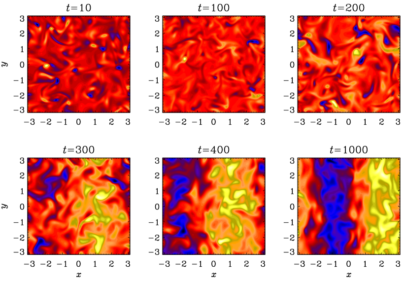
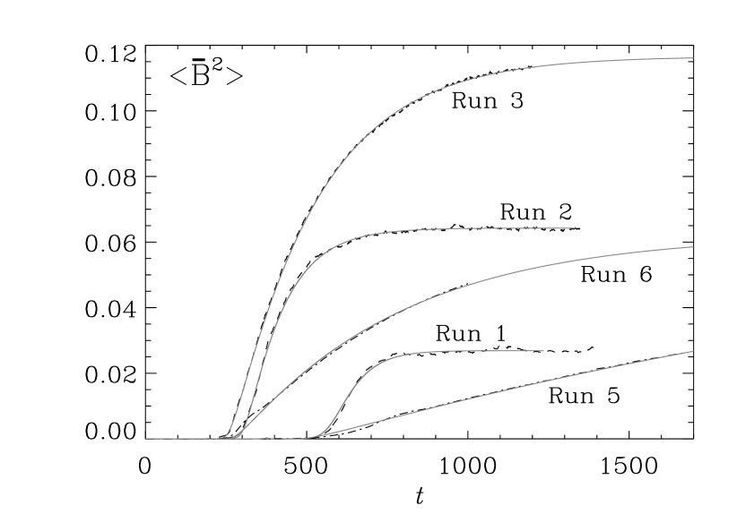
In the simulations of B01 the flow was forced at an intermediate wavenumber, , while the smallest wavenumber in the computational domain corresponds to . The kinetic energy spectrum peaks at , which is therefore also the wavenumber of the energy carrying scale. The turbulence is nearly fully helical with . The initial field is random, but as time goes on it develops a large scale component at wavenumber ; see Fig. 1. In Fig. 2 we show the evolution of the magnetic energy of the mean field from the same simulation.111Here the time unit is , where is the isothermal speed of sound, and the magnetic field is measured in units of . Here the mean field is defined as two-dimensional averages over planes perpendicular to the direction in which the mean field varies. There are of course three such directions, but there is usually only one direction for which there is a significant mean field.
While the saturation field strength increases with increasing magnetic Reynolds number, the time scale on which this nonlinear dynamo saturates increases too. To avoid misunderstandings, it is important to emphasize that this result applies only when we are in the nonlinear regime and when the flows are helical.
In turbulence one is used to situations where the microscopic values of viscosity and magnetic diffusivity do not matter in the sense that, for almost all practical purposes, they are superseded by turbulent effective values, and , respectively. This is because in turbulence there is spectral energy all the way down to the viscous/resistive length scale, , where is the turnover time.222The turnover time at the wavenumber is . Using Kolmogorov scaling, , one finds the familiar formula , where is the wavenumber of the energy carrying eddies. Thus, even when is very small, the rate of viscous dissipation, , is in general finite ( is the trace-less rate of strain tensor). Likewise, even when is very small, the rate of Joule dissipation, , is in general finite ( is the magnetic permeability). This is because the current density diverges with decreasing like , so the energy dissipation stays finite and asymptoticly independent of how small is. The trouble is that the value of magnetic helicity dissipation is proportional to (see below), and in the limit we have , so resistive magnetic helicity dissipation becomes impossible in the limit of large . In the following section we derive and discuss the evolution equation for magnetic helicity.
3 Magnetic helicity evolution
3.1 The two-scale property of helical turbulence
Usually in mean field dynamo theory one talks about the two-scale assumption made in order to derive the mean field equations (e.g. Moffatt 1978, Krause & Rädler 1980). This has to do with the fact that higher order derivatives in the mean field equation can only be neglected when the mean field is sufficiently smooth. Here, instead, we use the two-scale properties of helical turbulence as demonstrated in the previous section. These properties emerge automatically when the size of the whole body is at least several times larger than the scale of the turbulent eddies. As Fig. 1 shows explicitly, a large scale field (wavenumber ) emerges in addition to the forcing scale (wavenumber ).
In this section we discuss the magnetic helicity equation and use it together with the two-scale property of helical turbulence to derive the so-called magnetic helicity constraint that allows the result of Fig. 2 to be understood quantitatively.
3.2 Definition of helicity
The helicity of any solenoidal vector field , i.e. with , is defined as the volume integral of dotted with its inverse curl, i.e. . As pointed out by Moffatt (1969), the helicity quantifies the topological linkage between tubes in which is non-vanishing. In the following the linkage aspect of helicity will not be utilized, but rather the mathematical evolution equation that the helicity obeys (see the next section). However, the calculation of is problematic because it involves a gauge ambiguity in that the curl of also gives the same .
In the special case of periodic boundary conditions or for on the boundaries, where is the normal vector on the boundary, the helicity is actually gauge-invariant, because
| (1) | |||||
where we have used . Since the magnetic field is divergence free, the magnetic helicity, is gauge invariant. For other boundary conditions this is unfortunately not the case.
For vector fields whose inverse curl is a physically meaningful quantity, such as the vorticity , whose inverse curl is the velocity , the gauge question never arises. In this and similar cases the helicity density, in this case, is physically meaningful. Other examples are the cross helicity, , which describes the linkage between magnetic flux tubes and vortex tubes, and the current helicity, , which quantifies the linkage of current tubes. In these two cases it is natural to use and . For the magnetic field one can define the magnetic vector potential, , but is not a physically meaningful quantity and hence the magnetic helicity,
| (2) |
is gauge-dependent, unless the boundaries of the volume are periodic or perfectly conducting. Here and below, angular brackets denote volume averages. Occasionally, however, we simply refer to as the magnetic helicity, but this is strictly speaking only the magnetic helicity per unit volume.
In the following section we derive the evolution equation for and focus first on the case where the boundary conditions are indeed periodic, so is gauge-invariant.
3.3 Derivation of the magnetic helicity equation
The homogeneous Maxwell equations are
| (3) |
Expressing this in terms of the magnetic vector potential, , where , we have
| (4) |
where is the scalar potential. Dotting Eqs (3) and (4) with and , respectively, and adding them, we have
| (5) |
Here, is the magnetic helicity density, but since it is not gauge invariant (see below) it is not a physically meaningful quantity. After integrating Eq. (5) over a periodic volume, the divergence term does not contribute. Furthermore, using Ohm’s law, , where is the current density, we have
| (6) |
i.e. the magnetic helicity, , changes only at a rate that is proportional to . (Here and elsewhere, angular brackets denote volume averaging.) As discussed in the previous section, this rate converges to zero in the large limit. Here, angular brackets denote volume averages, i.e. .
We recall that for periodic boundary conditions, is invariant under the transformation , which does not change the value of . Here, is a gauge potential. Thus, for periodic boundary conditions, is a physically meaningful quantity. The same is also true for perfectly conducting boundaries (see Brandenburg & Dobler 2002 for corresponding simulations). For open boundaries, however, is not gauge invariant, but one can derive a gauge-invariant relative magnetic helicity (Berger & Field 1984).
3.4 The magnetic helicity constraint
A very simple argument can be made to explain the saturation level and the resistively slow saturation behavior observed in Fig. 2. The only assumption is that the turbulence is helical, i.e. , where is the vorticity, and that this introduces current helicity , at the same scale and of the same sign as the kinetic helicity. Here we have split the field into large and small scale fields, i.e. and hence also and .
The first remarkable thing to note is that, even though we are dealing with helical dynamos, there is no net current helicity in the steady state, i.e.
| (7) |
see Eq. (6). However, using the decomposition into large and small scale fields, we can write
| (8) |
so we have
| (9) |
in the steady state. We now introduce the approximations333Here and elsewhere we use units where or, following R. Blandford (private communication), we use units in which pi is one quarter.
| (10) |
where and are the typical wavenumbers of the mean and fluctuating fields, respectively. These approximations are only valid for fully helical turbulence, but can easily be generalized to the case of fractional helicity; see Sect. 4.1 and Blackman & Brandenburg (2002, hereafter BB02). We have furthermore assumed that the sign of the kinetic helicity is negative, as is the case in the northern hemisphere of the sun, for example. (The case of positive kinetic helicity is straightforward; see below.) The wavenumber of the fluctuating field is for all practical purposes equal to the wavenumber of the forcing function. (In more general situations, such as convection or shear flow turbulence, would be the wavenumber of the energy carrying eddies.) We also note that for large values of the magnetic Reynolds number, , the factor in Eq. (10) gets attenuated by an factor (BB02). On the other hand, the wavenumber of the mean field is in practice the wavenumber of the box, i.e. . Inserting now Eq. (10) into (9) yields
| (11) |
i.e. the energy of the mean field can exceed the energy of the fluctuating field – in contrast to earlier expectations (e.g. Vainshtein & Cattaneo 1992, Kulsrud & Andersen 1992, Gruzinov & Diamond 1994). Indeed, in the two-dimensional case there is an exact result due to Zeldovich (1957),
| (12) |
This result has also be derived in three dimensions using first order smoothing (Krause & Rädler 1980), but it is important to realize that this result can break down in the nonlinear case in three dimensions, where Eq. (11) is in good agreement with the simulations results. However, the assumption of periodic or closed boundaries is an essential one. We return to the more general case in Sects 4.4–4.5.
The time dependence near the saturated state can be approximated by using
| (13) |
These equations are still valid in the case of fractional helicity (BB02). Only the two-scale assumption is required. Near saturation,
| (14) |
i.e. and so we can neglect , and the magnetic helicity equation (6) becomes therefore an approximate evolution equation for the magnetic helicity of the mean field,
| (15) |
or, by using Eq. (10),
| (16) |
Note the plus sign in front of the term resulting from Eq. (10). The plus sign leads to growth while the minus sign in front of the term leads to saturation (but both terms are proportional to the microscopic value of ; see below). Once the small scale field has saturated, which will happen after a few dynamical time scales such that , the large scale field will continue to evolve slowly according to
| (17) |
where is the time at which has reached approximate saturation. In practice, can be determined such that Eq. (17) describes the simulation data best. We refer to Eq. (17) as the magnetic helicity constraint. The agreement between this and the actual simulations (Fig. 3) is quite striking.

The significance of this remarkable and simple equation and the almost perfect agreement with simulations is that the constraint can be extrapolated to large values of where it would provide a benchmark, against which all analytic dynamo theories, when subjected to the same periodic boundary conditions, should be compared to. In particular the late saturation behavior should be equally slow. We return to this in Sect. 5.
An important question is whether anything can be learned about stars and galaxies. Before this can be addressed, we need to understand the differences between dynamos in real astrophysical bodies and dynamos in periodic domains.
4 What do stars and galaxies do differently?
We begin with a discussion of fractional helicity, shear and other effects that cause the magnetic helicity to be reduced. We then address the possibility of helicity fluxes through boundaries, which can alleviate the helicity constraint (Blackman & Field 2000).
4.1 Fractional helicity
When the turbulence is no longer fully helical, Eq. (10) is no longer valid and needs to be generalized to
| (18) |
where and are coefficients denoting the degree to which the mean and fluctuating fields are helical. Equation (13) is still approximately valid in the fractionally helical case.
Maron & Blackman (2002) found that there is a certain threshold of below which the large scale dynamo effect stops working. Qualitatively, this could be understood by noting that the large scale magnetic field comes from the helical part of the flow, so the velocity field can be though of as having a helical and a nonhelical component, i.e.
| (19) |
However, the dynamo effect has to compete with turbulent diffusion which comes from both the helical and the nonhelical parts of the flow. Thus, when becomes too large compared with the large scale dynamo effect will stop working.
Although we have not yet discussed mean field theory we may note that the value of the threshold can be understood quantitatively (Brandenburg et al. 2002, hereafter BDS02) and one finds that large scale dynamo action is only possible when
| (20) |
In many three-dimensional turbulence simulations or in astrophysical bodies, this threshold criterion may not be satisfied, and so mean field dynamo of the type described above ( dynamo) may not be excited. If there is shear, however, this criterion will be modified to
| (21) |
where is the degree to which the large scale field is helical. In dynamos with strong shear, may be very small, making mean field dynamo action in fractionally helical flows more likely. This will be discussed in the next section.
4.2 Dynamos with shear
In the presence of shear, the streamwise component of the field can be amplified by winding up the poloidal (cross-stream) field. Again, the resulting saturation field strength can be estimated based on magnetic helicity conservation arguments.
Note first of all that for closed or periodic domains, Eq. (8) is still valid and therefore in the steady state.444This is because in the term in the magnetic helicity equation the induction term, , drops out after dotting with . (For this reason, also ambipolar diffusion and the Hall effect do not change magnetic helicity conservation.) However, while still depends on the helicity of the small scale field, the corresponding value of no longer provides such a stringent bound on as before. This is because shear can amplify the toroidal field independently of any magnetic helicity considerations. The component of that is amplified by shear is nonhelical and so we have
| (22) |
(or at least when the helicity of the forcing is negative and therefore negative). The value of is proportional to the ratio of poloidal to toroidal field
| (23) |
where the numerical pre-factor can be different for different examples.555Take as an example for , so and and therefore . With these preparations the magnetic helicity constraint can be generalized to
| (24) |
This form of the constraint was proposed and confirmed using three-dimensional simulations of forced helical turbulence with large scale shear (Brandenburg et al. 2001, hereafter BBS01); see also Fig. 4.
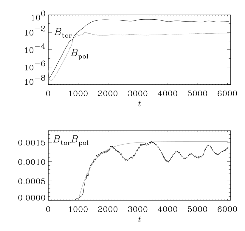
The main conclusion to be drawn from this is that the magnetic helicity constraint is still valid in the presence of shear, i.e. the timescale of saturation is still controlled by the microscopic magnetic diffusivity. The only difference is that stronger field strengths are now possible.
Another interesting aspect is that dynamos with shear allow for oscillatory solutions of the magnetic field. This is expected from mean field dynamo theory (Steenbeck & Krause 1969a,b), but it is also borne out by simulations (BBS01). The main result is that the resulting cycle frequency seems to scale with the microscopic magnetic diffusivity, not the turbulent magnetic diffusivity. This confirms again that in a closed domain the magnetic helicity constraint plays a crucial role in controlling the timescale of nonlinear dynamos.
4.3 Hall effect dynamos
In recent years the importance of the Hall effect has been emphasized by a number of groups, especially in applications to protostellar accretion discs (Balbus & Terquem 2001). The hall effect can lead to strong nonlinear steepening of field gradients (Vainshtein et al. 2000), and is therefore important for fast reconnection (e.g. Rogers et al. 2001), which in turn is relevant for neutron stars (Hollerbach & Rüdiger 2004). Nevertheless, since magnetic helicity generation (and removal) is proportional to the dot product of electric and magnetic fields, and since the Hall current is proportional to , the Hall term does not affect magnetic helicity conservation. Therefore the resistively limited saturation behavior should not be affected by the Hall term. Nevertheless, some degree of extra field amplification of the large scale field has been reported (Mininni et al. 2003), and it will be interesting to identify exactly the processes that led to this amplification.
4.4 Magnetic helicity exchange across the equator or with depth
The presence of an equator provides a source of magnetic helicity exchange between domains of negative helicity in the northern hemisphere (upper disc plane in an accretion disc) and positive helicity in the southern hemisphere (lower disc plane). A similar situation can also arise in convection zones where the helicity is expected to change with depth (Yoshimura 1975).
So far, simulations have not yet shown that the losses of small scale magnetic fields are actually stronger than those of large scales fields. In Fig. 5 we show the saturation behavior of a system that is periodic, but the helicity of the forcing is modulated in the -direction such that the sign of the kinetic helicity changes in the middle. One can therefore view this system as two subsystems with a boundary in between. This boundary would correspond to the equator in a star or the midplane in a disc. It can also model the change of sign of helicity at some depth in a convection zone.

As far as the magnetic helicity constraint is concerned, the divergence term of current helicity flux is likely to be important when there is a boundary between two domains with different helicities. Naively, one might expect there to be current helicity fluxes that are proportional to the current helicity gradient, analogous to Fick’s diffusion law. These current helicity fluxes should be treated separately for large and small scale components of the field, so we introduce approximations to the current helicity fluxes from the mean and fluctuating fields as
| (25) |
The rate of magnetic helicity loss is here proportional to some turbulent diffusivity coefficient, or for the losses from mean or fluctuating parts, respectively. We assume that the small and large scale fields are maximally helical (or have known helicity fractions and ) and have opposite signs of magnetic helicity at small and large scales. The details can be found in BDS02 and Blackman & Brandenburg (2003). The strength of this approach is that it is quite independent of mean field theory.
We proceed analogously to the derivation of Eq. (17) where we used the magnetic helicity equation (6) for a closed domain to estimate the time derivative of the magnetic helicity of the mean field by neglecting the time derivative of the fluctuating field. This is a good approximation after the fluctuating field has reached saturation, i.e. . Thus, we have
| (26) |
where corresponds to the case of a closed domain. Note also that we have here ignored the volume integration, so we are dealing with horizontal averages that depend still on height and on time.
After the time when the small scale magnetic field saturates, i.e. when , we have . After that time, Eq. (26) can be solved to give
| (27) |
This equation demonstrates three remarkable properties (Brandenburg et al. 2003, Brandenburg & Subramanian 2004):
-
•
Large scale helicity losses are needed () to shorten the typical time scale. This is required to prevent resistively long cycle periods.
-
•
However, the saturation amplitude is proportional to , so the large scale field becomes weaker as is increased. Thus,
-
•
also small scale losses are needed to prevent the saturation amplitude from becoming too small.
Future work can hopefully verify that these conditions are indeed obeyed by a working large scale dynamo. Simulations without shear have been unsuccessful to demonstrate that small scale losses are important (Brandenburg & Dobler 2001), but new simulations with shear now begin to show significant small scale losses of current helicity, an enhanced effect (Brandenburg & Sandin 2004), and strong large scale dynamo action (see below).
4.5 Open surfaces and shear
The presence of an outer surface is in many respects similar to the presence of an equator. In both cases one expects magnetic and current helicity fluxes via the divergence term. A particularly instructive system is helical turbulence in an infinitely extended horizontal slab with stress-free boundary conditions and a vertical field condition, i.e.
| (28) |
Such simulations have been performed by Brandenburg & Dobler (2001) who found that a mean magnetic field is generated, similar to the case with periodic boundary conditions, but that the energy of the mean magnetic field, , decreases with magnetic Reynolds number. Nevertheless, the energy of the total magnetic field, , does not decrease with increasing magnetic Reynolds number. Although they found that decreases only like , new simulations confirm that a proper scaling regime has not yet been reached and that the current data may well be compatible with an dependence; see Fig. 6.

Clearly, an asymptotic decrease of the mean magnetic field must mean that the small scale dynamo does not work with such boundary conditions. Thus, the anticipated advantages of open boundary conditions are not borne out by this type of simulations.

At this point we can mention some new simulations in a cartesian domain where differential rotation has been modeled as a region of the convection zone without explicitly allowing for convection; see Fig. 7. Instead, an external forcing term has been applied that also drives the differential rotation. (Studies of the effect have already been published; see Sect. 5.6 for details of the simulations and Sect. 5 for a discussion of the direct correspondence between the helicity constraint and the so-called catastrophic quenching.) Here we briefly report on recent explicit dynamo simulations that have been carried out in this geometry.
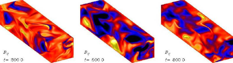
The size of the computational domain is and the numerical resolution is meshpoints. The magnetic Reynolds number based on the forcing wavenumber and the turbulent flow is around 80 and shear flow velocity exceeds the rms turbulent velocity by a factor of about 5. We have carried out experiments with no helicity in the forcing (labeled by ), as well as positive and negative helicity in the forcing (labeled by and , respectively); see Fig. 8 for a visualization of the run without kinetic helicity. We emphasize that no explicit effect has been invoked. The labeling just reflects the fact that, in isotropic turbulence, negative kinetic helicity (as in the northern hemisphere of a star or the upper disc plane in galaxies) leads to a positive effect, and vice versa.

We characterize the relative strength of the mean field by the ratio , where overbars denote an average in the toroidal () direction; see Fig. 9. There are two surprising results emerging from this work. First, in the presence of shear rather strong mean fields can be generated, where up to 70% of the energy can be in the mean field; see Fig. 9. Second, even without any kinetic helicity in the flow there is strong large scale field generation. Obviously, this cannot be an dynamo in the usual sense. One possibility is the effect, which emerged originally in the presence of the Coriolis force; see Rädler (1969) and Krause & Rädler (1980). In the present case with no Coriolis force, however, a effect is possible even in the presence of shear alone, because the vorticity associated with the shear contributes directly to (Rogachevskii & Kleeorin 2003).
There is evidence that the strong dynamo action seen in the simulations is only possible due to the combined presence of open boundaries and shear. This however has so far only been checked explicitly for the effect that is present when the forcing is helical; see Sect. 5.6. In the case of the solar surface such losses are actually observed to occur in the form of coronal mass ejections and in active regions. In the sun, coronal mass ejections are quite vigorous events that are known to shed large amounts of helical magnetic fields (Berger & Ruzmaikin 2000, DeVore 2000, Chae 2000, Low 2001). This kind of physics is not at all represented by adopting vacuum or pseudo-vacuum (vertical field) boundary conditions, as was done in Brandenburg & Sandin (2004).
5 Connection with the effect
5.1 Preliminary considerations
The effect formalism provides so far the only workable mathematical framework for describing the large scale dynamo action seen in simulations of helically forced turbulence. (In this section we retain the factor.) The governing equation for the mean magnetic field is
| (29) |
where is the electromotive force resulting from the nonlinearity in the averaged Ohm’s law. Without mean flow, , and an electromotive force given by a homogeneous isotropic effect and turbulent diffusion , i.e.
| (30) |
we have
| (31) |
which has solutions of the form with the dispersion relation
| (32) |
and three possible eigenfunctions (appropriate for the periodic box)
| (33) |
where . Obviously, when the coefficients and remain constant, and there is an exponentially growing solution (for ), the solution must eventually grow beyond any bound. At the latest when the magnetic field reaches equipartition with the kinetic energy, and must begin to depend on the magnetic field itself. However, the present case is sufficiently simple so that we can continue to assume that , as well as and , are uniform in space and depend only on time.
Comparison with simulations has enabled us to eliminate a large number of various quenching models where . The only quenching model that seems reasonably well compatible with simulations of -like dynamo action in a periodic box without shear is
| (34) |
see Fig. 3. However, this type of quenching is not fully compatible with magnetic helicity conservation, as has been shown by Field & Blackman (2002). This will be discussed in the next section.
5.2 Dynamical quenching
The basic idea is that magnetic helicity conservation must be obeyed, but the presence of an effect leads to magnetic helicity of the mean field which has to be balanced by magnetic helicity of the fluctuating field. This magnetic helicity of the fluctuating (small scale) field must be of opposite sign to that of the mean (large scale) field.
We begin with the uncurled mean-field induction equation, written in the form
| (35) |
dot it with , add the result to , average over the periodic box, and obtain
| (36) |
To satisfy the helicity equation for the full field, , we must have
| (37) |
Note the minus sign in front of the term, indicating once again that the effect produces magnetic helicity of opposite sign at the mean and fluctuating fields. The sum of the two equations yields Eq. (6).
The significance of Eq. (37) is that it contains the term which contributes to the effect, as was first shown by Pouquet et al. (1976). Specifically, they found (see also Blackman & Field 2002)
| (38) |
where is the correlation time of the turbulence, is the vorticity, and is the kinematic helicity.
Using , see Eq. (13), we can rewrite Eq. (37) in a form that can directly be used in mean field calculations:
| (39) |
Here we have used to eliminate in favor of and to eliminate in favor of .
So, is no longer just an algebraic function of , but it is related to via a dynamical, explicitly time-dependent equation. In the context of dynamos in periodic domains, where magnetic helicity conservation is particularly important, the time dependence of can hardly be ignored, unless one wants to describe the final stationary state, which can be at the end of a very slow saturation phase. However, in order to make contact with earlier work, it is useful to consider the stationary limit of Eq. (39), i.e. set .
5.3 Steady limit and its limitations
In the steady limit the term in brackets in Eq. (39) can be set to zero, so this equation reduces to
| (40) |
Solving this equation for yields (Kleeorin & Ruzmaikin 1982, Gruzinov & Diamond 1994)
| (41) |
And, sure enough, for the numerical experiments with an imposed large scale field over the scale of the box (Cattaneo & Hughes 1996), where is spatially uniform and therefore , one recovers the ‘catastrophic’ quenching formula,
| (42) |
which implies that becomes quenched when for the sun, and for even smaller fields in the case of galaxies.
On the other hand, if the mean field is not imposed, but maintained by dynamo action, cannot be spatially uniform and then is finite. In the case of a Beltrami field (33), is some effective wavenumber of the large scale field [; see Eq. (22)]. Since enters both the numerator and the denominator, tends to , i.e.
| (43) |
Compared with the kinematic estimate, , is only quenched by the modified scale separation ratio. More importantly, is quenched to a value that is just slightly above the critical value for the onset of dynamo action, . How is it then possible that the fit formula (34) for and produced reasonable agreement with the simulations? The reason is that in the simple case of an dynamo the solutions are degenerate in the sense that and are parallel to each other. Therefore, the term is the same as , which means that in the mean EMF the term , where is given by Eq. (41), has a component that can be expressed as being parallel to . In other words, the roles of turbulent diffusion (proportional to ) and effect (proportional to ) cannot be disentangled. This is the force-free degeneracy of dynamos in a periodic box (BB02). This degeneracy is also the reason why for dynamos the late saturation behavior can also be described by an algebraic (non-dynamical, but catastrophic) quenching formula proportional to for both and , as was done in B01. To see this, substitute the steady state quenching expression for , from Eq. (41), into the expression for . We find
| (44) |
which shows that in the force-free case the adiabatic approximation, together with constant (unquenched) turbulent magnetic diffusivity, becomes equal to the pair of expressions where both and are catastrophically quenched. This force-free degeneracy is lifted in cases with shear or when the large scale field is no longer fully helical (e.g. in a nonperiodic domain, and in particular in the presence of open boundaries).
5.4 The Keinigs relation and its relevance
Applying Eq. (37) to the steady state using (and retaining factor), we get
| (45) |
where we have defined an effective wavenumber of the large scale field, ; see Eq. (9). This relation applies only to a closed or periodic box, because otherwise there would be boundary terms. Moreover, if the mean field is defined as a volume average, i.e. , then , so and one has simply
| (46) |
This equation is due to Keinigs (1983). For the more general case with this equation has been discussed in more detail by Brandenburg & Sokoloff (2002) and Brandenburg & Matthaeus (2004).
Let us now discuss the significance of this relation relative to Eq. (41). Both equations apply only in the strictly steady state, of course. Since we have assumed stationarity, we can replace by ; see Eq. (9). Thus, Eq. (45) reduces to
| (47) |
where is the total (turbulent and microscopic) magnetic diffusivity. This relation is just the condition for a marginally excited dynamo; see Eq. (32), so it does not produce any independent estimate for the value of . In particular, it does not provide a means of independently testing Eq. (41). The two can however be used to calculate the mean field energy in the saturated state and we find (BB02)
| (48) |
By replacing by an effective value , this equation can be generalized to apply also to the case with shear (for details see BB02).
5.5 Blackman’s multi-scale model: application to helical turbulence with imposed field
The restriction to a two scale model may in some cases turn out to be insufficient to capture the variety of scales involved in astrophysical bodies. This is already important in the kinematic stage when the small scale dynamo obeys the Kazantsev (1968) scaling with a spectrum that peaks at the resistive scale. As the dynamo saturates, the peak moves to the forcing scale. This lead Blackman (2003) to develop a four scale model where he includes, in addition to the wavenumbers of the mean field () and the wavenumber of the energy carrying scale of the velocity fluctuations (), also the viscous wavenumber () and the resistive wavenumber (). The set of helicity equations for the four different scales is
| (49) | |||||
| (50) | |||||
| (51) | |||||
| (52) |
where is the usual electromotive force based on kinetic helicity at the forcing scale, , with feedback proportional to , and has no kinetic helicity input but only reacts to the automatically generated magnetic helicity produced at the viscous scale . These equations are constructed such that
| (53) |
which is consistent with the magnetic helicity equation (6) for the total field. An important outcome of this model is that in the limit of large the magnetic peak travels from to on a dynamical timescale, i.e. a timescale that is independent of .
Brandenburg & Matthaeus (2004) have applied the general idea to the case of a model with an applied field. Here the new scale is the scale of the applied field, but since this scale is infinite, this field is fixed and not itself subject to an evolution equation. Nevertheless, the electromotive force from this field acts as a sink on the next smaller scale with wavenumber , which is the largest wavenumber in the domain of the simulation. They thus arrive at the following set of evolution equations,
| (54) | |||||
| (55) | |||||
| (56) |
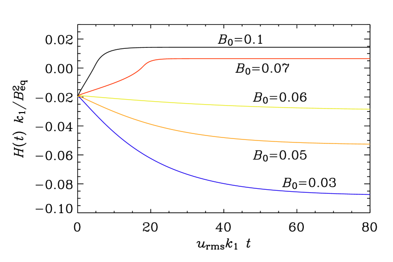
The square brackets around the first equation indicate that this equation is not explicitly included. From the second equation (55) one can see that there is a competition between two opposing effects: the effect operating on the imposed field and the effect operating on the field on the scale of the box. When the imposed field exceeds a certain field strength, , the former will dominate, reversing the sign of the magnetic helicity at wavenumber . This is actually seen in the simulations of helically forced turbulence with an imposed field ; see Fig. 10. We return to this at the end of this section.
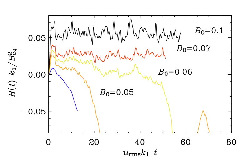
The work of Brandenburg & Matthaeus (2004) was motivated by earlier work of Montgomery et al. (2002) and Milano et al. (2003) who showed that, if the imposed magnetic field is weak or absent, there is a strong nonlocal transfer of magnetic helicity and magnetic energy from the forcing scale to larger scales. This leads eventually to the accumulation of magnetic energy at the scale of the box (Meneguzzi et al. 1981, Balsara & Pouquet 1999, B01). As the strength of the imposed field (wavenumber ) is increased, the accumulation of magnetic energy at the scale of the box () becomes more and more suppressed (Montgomery et al. 2002).
In order to solve the model equations, we have to make some assumptions about the electromotive force operating at and . The large scale magnetic helicity production from the effect operating on the imposed field is . On the other hand, at wavenumber is given by
| (57) |
To calculate in Eqs (55) and (56) we dot Eq. (57) with , volume average, and note that and . The latter relation assumes that the field at wavenumber is fully helical, but that it can have either sign. Thus, we have
| (58) |
The effects on the two scales are proportional to the residual magnetic helicity of Pouquet et al. (1976); see Eq. (38). In terms of and we write
| (59) |
| (60) |
for the effect with feedback from and , respectively.
For finite values of , the final value of is particularly sensitive to the value of and turns out to be too large compared with the simulations. This disagreement with simulations is readily removed by taking into account that should itself be quenched when becomes comparable to . Thus, we write
| (61) |
which is a good approximation to more elaborate expressions (Rüdiger & Kitchatinov 1993). We emphasize that this equation only applies to and is therefore distinct from Eqs. (34), (39), or (41).
Under the assumption that the turbulence is fully helical, the critical value of the imposed field can be estimated by balancing the two terms on the right hand side of Eq. (56) and by approximating, and . This yields
| (62) |
where the last equality is to be understood as a definition of the magnetic Reynolds number, see also BB02. For the sign of the magnetic helicity is the same both at and at , while for the signs are opposite.
In Fig. 11 we show the result of a numerical integration of Eqs (55) and (56). Both the three-dimensional simulation and the two-scale model show a similar value of , above which changes sign. This confirms the validity of our estimate of the critical value obtained from Eq. (62). Secondly, the time evolution is slow when and faster when . In the simulation, however, the field attains its final level for almost instantaneously, which is not the case in the model. The significance of this discrepancy remains unclear. Nevertheless, the level of agreement between the simulations and 3-scale model is surprising, suggesting that the approach can indeed be quite useful.
5.6 Alpha effect with open boundaries and shear
In a recent paper, Brandenburg & Sandin (2004) have carried out a range of simulations for different values of the magnetic Reynolds number, , for both open and closed boundary conditions using the geometry depicted on the right hand panel of Fig. 7. In order to measure , a uniform magnetic field, , is imposed, and the magnetic field is now written as . They have determined by measuring the turbulent electromotive force, and hence . Similar investigations have been done before both for forced turbulence (Cattaneo & Hughes 1996, B01) and for convective turbulence (Brandenburg et al. 1990, Ossendrijver et al. 2001).
As expected, is negative when the helicity of the forcing is positive, and changes sign when the helicity of the forcing changes sign. The magnitudes of are however different in the two cases: is larger when the helicity of the forcing is negative. In the sun, this corresponds to the sign of helicity in the northern hemisphere in the upper parts of the convection zone. This is here the relevant case, because the differential rotation pattern of the present model also corresponds to the northern hemisphere.
There is a striking difference between the cases with open and closed boundaries which becomes particularly clear when comparing the averaged values of for different magnetic Reynolds numbers; see Fig. 12. With closed boundaries tends to zero like , while with open boundaries shows no such decline. There is also a clear difference between the cases with and without shear together with open boundaries in both cases. In the absence of shear (dashed line in Fig. 12) declines with increasing , even though for small values of it is larger than with shear. The difference between open and closed boundaries will now be discussed in terms of a current helicity flux through the two open open boundaries of the domain.

5.7 Current helicity flux
It is suggestive to interpret the above results in terms of the dynamical quenching model. However, Eq. (39) has to be generalized to take the divergence of the flux into account. In order to avoid problems with the gauge, it is advantageous to work directly with instead of . Using the evolution equation, , for the fluctuating magnetic field, where is the small scale electric field and the mean electric field, one can derive the equation
| (63) |
where
| (64) |
is the current helicity flux from the small scale field, and the curl of the small scale current density, . In the isotropic case, , where is the typical wavenumber of the fluctuations, here assumed to be the forcing wavenumber. Ignoring the effect of the mean flow on [as is usually done; but see Krause & Rädler (1980) and the recent on the shear current effect by Rogachevskii & Kleeorin (2003, 2004); see Sect. 4.5], we obtain
| (65) |
where we have used and . Using standard expressions for the turbulent magnetic diffusivity, , and the equipartition field strength, , we eliminate via
| (66) |
This leads to an explicitly time dependent formula for ,
| (67) |
This equation is similar to that of Kleeorin et al. (2000, 2002, 2003) who considered the flux of magnetic helicity instead of current helicity.
Making use of the adiabatic approximation, i.e. putting the rhs of Eq. (67) to zero, one arrives at the algebraic steady state quenching formula ()
| (68) |
In the absence of a mean current, e.g. if the mean field is defined as an average over the whole box, then , and , so Eq. (68) reduces to
| (69) |
This expression applies to the present case, because we consider only the statistically steady state and we also define the mean field as a volume average.
For closed boundaries, , and so Eq. (69) clearly reduces to a catastrophic quenching formula, i.e. vanishes in the limit of large magnetic Reynolds numbers as
| (70) |
The dependence is confirmed by the simulations (compare with the dash-dotted line in Fig. 12). On the other hand, for open boundaries the limit gives
| (71) |
which shows that losses of negative helicity, as observed in the northern hemisphere of the sun, would enhance a positive effect (Kleeorin et al. 2000). In the simulations, the current helicity flux is found to be independent of the magnetic Reynolds number. This explains why the effect no longer shows the catastrophic dependence (see Fig. 12). In principle it is even conceivable that with a current helicity flux can be generated, for example by shear, and that this flux divergence could drive a dynamo, as was suggested by Vishniac & Cho (2001). It is clear, however, that for finite values of this would be a non-kinematic effect requiring the presence of an already finite field (at least of the order of ). This is because of the term in the denominator of Eq. (69). At the moment we cannot say whether this is perhaps the effect leading to the nonhelically forced turbulent dynamo discussed in Sect. 4.5, or whether it is perhaps the or shear-current effect that was also mentioned in that section.
6 What about quenching?
As we have seen above, in a closed domain the value of in the saturated state cannot conclusively be determined without also determining at the same time the turbulent magnetic diffusivity. There are different ways of determining . The values are not necessarily all in agreement with each other, because one does not know whether the mean field equation, where enters, is correct and applicable. We report here a few different examples where has been determined.
6.1 Direct measurements in a working dynamo
We first consider the case of a helical turbulent dynamo without shear (B01) and compare it with a simple mean-field dynamo. Assuming that is uniform, we can use Eq. (31) and, assuming furthermore that (which is the case when the helicity of the forcing is positive, as in B01), the solution is
| (72) |
The time-dependent equations can then be written as
| (73) |
| (74) |
In an isotropic, homogeneous dynamo, the eigenfunction obeys .
We now assume that, at some particular time, we put , for example. This means that will first grow linearly in time at a rate that is proportional to like . At the same time as grows, will first decrease at a rate that is proportional to . This allows an independent estimate of and by solving the matrix equation
| (75) |
The result for is found to be roughly consistent with that of Cattaneo & Hughes (1996), and the result for is reproduced in Fig. 13, and can be described by the fit formula
| (76) |
with . This expression needs to be compared with that obtained from other approaches.

The fact that the results obtained for by using this approach are consistent with that for a uniform field is quite surprising and unexpected. This agreement probably indicates that in this type of simulation is independent of scale – at least in the scale range corresponding to wavenumbers () and . In general, this may not be true. Indeed, in the case of accretion discs some numerical evidence for scale dependence of and has been found (Brandenburg & Sokoloff 2002).
6.2 Measurements in an dynamo
In the case of an dynamo the cycle frequency depends directly on the nonlinearly suppressed value of
| (77) |
see BB02 (their Sect. 4.2). The estimates of BBS01 indicated that the dynamo numbers based on shear, , is between 40 and 80, whilst the total dynamo number () is between 10 and 20 (see BBS01), and hence . Thus, shear dominates strongly over the effect ( is between 150 and 300), which is typical for -type behavior (i.e. oscillations) rather than -type behavior which would start when is below about 10 (e.g. Roberts & Stix 1972).
The results shown in Table LABEL:Tao2 suggest that the period in this oscillatory dynamo is controlled by the microscopic magnetic diffusivity, because is approximately independent of . Using Eq. (77), this means that for between 30 and 200. This result would favor a model where is still quenched in an -dependent fashion. In the next section we show that the apparent -dependent quenching can easily also be produced when the field possesses a helical component.
Run (i) (ii) (iii) 5 10 25 30 80 200 1000 2000 4000 4 6 20 20 30 60 0.11 0.06 0.014 8…9 6…12
Looking at the scaling of the cycle frequency with resistivity may be quite misleading in the present case, because the large scale magnetic field exceeds the kinetic energy by a large factor (20–30). This would always lead to the usual (non-catastrophic) quenching of and . Furthermore, such strong magnetic fields will affect the mean shear flow. Most important is perhaps the fact that in the simulation of BBS01 the shear flow varies sinusoidally in the cross stream direction, so the mean field depends on the two coordinate directions perpendicular to the streamwise direction. For this reason BB02 solved the mean field and dynamical quenching equations in a 2-dimensional model. It turned out to be important to allow for non-catastrophic quenching of using Eq. (76) where the value of has been varied between 0 and 3. The asymptotic behavior (as opposed to , for example) was motivated both by simulations (B01) and analytic results (Kitchatinov et al. 1994, Rogachevskii & Kleeorin 2001).
In order to see whether the models can be made to match the direct simulations, several input parameters were varied. It should be kept in mind, however, that not all input parameters are well known. This has to do with the uncertainty in the correspondence between the magnetic Reynolds number in the model (which measures ) and the simulations [where it is defined as ]. Likewise, the dynamo number is not well determined. Nevertheless, many of the output parameters are reasonably well reproduced; see Table LABEL:Tao3.
Model BBS01 1–2 – – 2000 6 30 0.014 0.06 0.008 0.015 R1 1.0 100 0 2000 0.20 15 0.031 0.065 0.016 0.044 AG2 0.5 20 3 2000 0.10 22 0.011 0.024 0.006 0.021 BDS02 1–2 – – 1000 4 20 0.018 0.11 0.014 0.006 s3 0.35 33 1 1000 0.07 6 0.029 0.061 0.014 0.016 S1 0.35 33 3 1000 0.07 19 0.009 0.019 0.005 0.016
6.3 Decay experiments
Finally, we consider the decay of a magnetic field. This provides a fairly straightforward method of determining from the decay rate of a sinusoidal field with wavenumber , so . The result reported by Yousef et al. (2003) suggests that
| (78) |
Once the mean flow profile has decreased below a certain level (), it cannot decay further and continues to fluctuate around , corresponding to the level of the rms velocity of the (forced!) turbulence at (see the dashed line in Fig. 14).

The quenching of the magnetic diffusivity, , can be obtained from one and the same run by simply determining the decay rate, , at different times, corresponding to different values of . To describe departures from purely exponential decay one can adopt a -dependent expression of the form (76). It turns out that the value of is not universal and depends on the field geometry. This is easily demonstrated by comparing the decay of helical and nonhelical initial fields; see Fig. 15.
In the next section we show that the slower decay of , and hence the implied stronger quenching of , can also be described by a self-induced magnetic effect which acts such as to decrease the decay rate. In the case of a helical initial field, we have , i.e. the large scale field is force-free and interacts only weakly with the turbulence.

Thus, the indications here are that for non-helical fields, is not catastrophically quenched. A resistively slow decay rate occurs however when the magnetic field is helical, but this is not to be explained by a catastrophically quenched , but by the magnetic effect, , that tries to keep the magnetic field as large as possible, just as enforced by the magnetic helicity constraint. The phenomenon, described in this way, may be more easily described in terms of helicity conservation, because the system has magnetic helicity that can only decay slowly on a resistive time scale, hence lowering the apparent turbulent diffusivity down to the microscopic value . This will be explained in more detail in the next section.
6.4 Taylor relaxation or selective decay
In the case of a helical field with the slow decay of is related to the conservation of magnetic helicity. As already discussed by BB02, this behavior is related to the phenomenon of selective decay (e.g. Montgomery et al. 1978) and can be described by the dynamical quenching model. This model applies even to the case where the turbulence is nonhelical and where there is no effect in the usual sense. However, the magnetic contribution to is still non-vanishing, because it is driven by the helicity of the large scale field.
To demonstrate this quantitatively, Yousef et al. (2003) have adopted the one-mode approximation () with , the mean-field induction equation
| (79) |
together with the dynamical -quenching formula (39),
| (80) |
where
| (81) |
is the electromotive force, and is defined as the ratio , which is expected to be close to the value of .

In Fig. 16 we show the evolution of for helical and nonhelical initial conditions, and , respectively. In the case of a nonhelical field, the decay rate is not quenched at all, but in the helical case quenching sets in for . In the helical case, the onset of quenching at is well reproduced by the simulations. In the nonhelical case, however, some weaker form of quenching sets in when (see the right hand panel of Fig. 15). We refer to this as standard quenching (e.g. Kitchatinov et al. 1994) which is known to be always present; see Eq. (76). BB02 found that, for a range of different values of , resulted in a good description of the simulations of cyclic -type dynamos (BDS02).
Yousef et al. (2003) also showed that the turbulent magnetic Prandtl number is indeed independent of the microscopic magnetic Prandtl number. The resulting values of the flow Reynolds number, , varied between 20 and 150, giving in the range between 0.1 and 1. Within plot accuracy the three values of turn out to be identical in the interval where the decay is exponential.
7 Conclusions
In the present review we have tried to highlight some of the recent discoveries that have led to remarkable advances in the theory of mean field dynamos. Of particular importance are the detailed confirmations of various aspects of mean field theory using helically forced turbulence simulations. The case of homogeneous turbulence with closed or periodic boundary conditions is now fairly well understood. In all other cases, however, the flux of current helicity becomes important. The closure theory of these fluxes is still a matter of ongoing research (Kleeorin et al. 2000, 2002, 2003), Vishniac & Cho (2001), Subramanian & Brandenburg (2004), and Brandenburg & Subramanian (2004). The helicity flux of Vishniac & Cho (2001) has been independently confirmed (Subramanian & Brandenburg 2004). A more detailed investigation of current helicity fluxes appears to be quite important when one tries to get qualitative and quantitative agreement between simulations and theory.
The presence of current helicity fluxes is particularly important when there is also shear. This was already recognized by Vishniac & Cho (2001) who applied their calculations to the case of accretion discs where shear is particularly strong. In the near future it should be possible to investigate the emergence of current helicity flux in more detail. This would be particularly interesting in view of the many observations of coronal mass ejections that are known to be associated with significant losses of magnetic helicity and hence also of current helicity (DeVore 2000, Démoulin et al. 2002, Gibson et al. 2002).
In order to be able to model coronal mass ejections it should be particularly important to relax the restrictions imposed by the vertical field conditions employed in the simulations of Brandenburg & Sandin (2004). A plausible way of doing this would be to include a simplified version of a corona with enhanced temperature and hence decreased density, making this region a low-beta plasma.
In the context of accretion discs the importance of adding a corona is well recognized (Miller & Stone 2000), although its influence on large scale dynamo action is still quite open. Regarding hydromagnetic turbulence in galaxies, most simulations to date do not address the question of dynamo action (Korpi et al. 1999, de Avillez & Mac Low 2002). This is simply because here the turbulence is driven by supernova explosions which leads to strong shocks. These in turn require large numerical diffusion, so the effective magnetic Reynolds number is probably fairly small and dynamo action may only be marginally possible. In nonhelically driven turbulence has been applied to the galactic medium to argue that it is dominated by small scale fields (Schekochihin et al. 2002), but the relative importance of small scale fields remains still an open question (Haugen et al. 2003). Galaxies are however rotating and vertically stratified, so the flows should be helical, but in order to say anything about magnetic helicity evolution, much larger magnetic Reynolds numbers are necessary. At the level of mean field theory the importance of magnetic helicity fluxes is well recognized. The explicitly time-dependent dynamical quenching equation with magnetic helicity fluxes has been included in mean field simulations (Kleeorin et al. 2000, 2002, 2003), but the form of the adopted fluxes is to be clarified in view of the differences with the results of Vishniac & Cho (2001) and Subramanian & Brandenburg (2004). Nevertheless, given that the form of the dynamical quenching equations is likely to be still incomplete, it remains to be demonstrated, using simulations, that magnetic or current helicity fluxes do really allow the dynamo to saturate on a dynamical time scale.
Acknowledgements
The Danish Center for Scientific Computing is acknowledged for granting time on the Horseshoe cluster. This work has been completed while being on sabbatical at the Isaac Newton Institute for Mathematical Sciences in Cambridge.
References
- (1) de Avillez, M. A., Mac Low, M.-M.: 2002, ApJ 581, 1047
- (2) Balbus, S. A., Terquem, C.: 2001, ApJ 552, 235
- (3) Balsara, D., Pouquet, A.: 1999, Phys. Plasmas 6, 89
- (4) Beck, R., Brandenburg, A., Moss, D., et al.: 1996, ARA&A 34, 155
- (5) Berger, M., Field, G. B.: 1984, JFM 147, 133
- (6) Berger, M. A., Ruzmaikin, A.: 2000, JGR 105, 10481
- (7) Boldyrev, S., Cattaneo, F.: 2004, Phys. Rev. Lett. 92, 144501
- (8) Blackman, E. G.: 2003, MNRAS 344, 707
- (9) Blackman, E. G., Field, G. F.: 2000, MNRAS 318, 724
- (10) Blackman, E. G., Field, G. B.: 2002, Phys. Rev. Lett. 89, 265007
- (11) Blackman, E. G., Brandenburg, A.: 2002, ApJ 579, 359 (BB02)
- (12) Blackman, E. G., Brandenburg, A.: 2003, ApJ 584, L99
- (13) Brandenburg, A.: 2001, ApJ 550, 824 (B01)
- (14) Brandenburg, A.: 2003, in Simulations of magnetohydrodynamic turbulence in astrophysics, ed. E. Falgarone, T. Passot (Lecture Notes in Physics, Vol. 614. Berlin: Springer), p. 402
- (15) Brandenburg, A., Dobler, W.: 2001, A&A 369, 329
- (16) Brandenburg, A., Dobler, W.: 2002, Comp. Phys. Comm. 147, 471
- (17) Brandenburg, A., Matthaeus, W. H.: 2004, Phys. Rev. E 69, 056407
- (18) Brandenburg, A., Sandin, C.: 2004, A&A 427, 13
- (19) Brandenburg, A., Sokoloff, D.: 2002, Geophys. Astrophys. Fluid Dyn. 96, 319
- (20) Brandenburg, A., Subramanian, K.: 2004, Phys. Rep. [arXiv:astro-ph/0405052]
- (21) Brandenburg, A., Bigazzi, A., Subramanian, K.: 2001, MNRAS 325, 685 (BBS01)
- (22) Brandenburg, A., Blackman, E. G., Sarson, G. R.: 2003, Adv. Spa. Sci. 32, 1835
- (23) Brandenburg, A., Dobler, W., Subramanian, K.: 2002, AN 323, 99 (BDS02)
- (24) Brandenburg, A., Nordlund, Å., Pulkkinen, P., et al.: 1990, A&A 232, 277
- (25) Brun, A. S., Miesch, M. S., Toomre, J.: 2004, ApJ 614, 1073
- (26) Cattaneo F., Hughes D. W.: 1996, Phys. Rev. E 54, R4532
- (27) Chae, J.: 2000, ApJ 540, L115
- (28) Cowling, T. G.: 1934, MNRAS 94, 39
- (29) Démoulin, P., Mandrini, C. H., van Driel-Gesztelyi, L., et al.: 2002, Sol. Phys. 207, 87
- (30) DeVore, C. R.: 2000, ApJ 539, 944
- (31) Field, G. B., Blackman, E. G.: 2002, ApJ 572, 685
- (32) Gibson, S. E., Fletcher, L., Del Zanna, G., et al.: 2002, ApJ 574, 1021
- (33) Gilman, P. A.: 1983, ApJS 53, 243
- (34) Glatzmaier, G. A.: 1985, ApJ 291, 300
- (35) Gruzinov, A. V., Diamond, P. H.: 1994, Phys. Rev. Lett. 72, 1651
- (36) Haugen, N. E. L., Brandenburg, A., Dobler, W.: 2003, ApJ 597, L141
- (37) Haugen, N. E. L., Brandenburg, A., Dobler, W.: 2004, Phys. Rev. E 70, 016308
- (38) Hollerbach, R., Rüdiger, G.: 2004, MNRAS 347, 1273
- (39) Hughes D. W., Cattaneo F., Kim E. J.: 1996, Phys. Lett. 223, 167
- (40) Kazantsev, A. P.: 1968, Sov. Phys. JETP 26, 1031
- (41) Keinigs, R. K.: 1983, Phys. Fluids 26, 2558
- (42) Kitchatinov, L. L., Rüdiger, G., Pipin, V. V.: 1994, AN 315, 157
- (43) Kleeorin, N. I., Ruzmaikin, A. A.: 1982, Magnetohydrodynamics 18, 116
- (44) Kleeorin, N. I, Moss, D., Rogachevskii, I., Sokoloff, D.: 2000, A&A 361, L5
- (45) Kleeorin, N. I, Moss, D., Rogachevskii, I., Sokoloff, D.: 2002, A&A 387, 453
- (46) Kleeorin, N. I, Moss, D., Rogachevskii, I., Sokoloff, D.: 2003, A&A 400, 9
- (47) Korpi, M. J., Brandenburg, A., Shukurov, A., et al.: 1999, ApJ 514, L99
- (48) Krause, F., Rädler, K.-H.: 1980, Mean-Field Magnetohydrodynamics and Dynamo Theory (Akademie-Verlag, Berlin; also Pergamon Press, Oxford)
- (49) Kulsrud, R. M., Anderson, S. W.: 1992, ApJ 396, 606
- (50) Kulsrud, R. M.: 1999, ARA&A 37, 37
- (51) Low, B. C.: 2001, JGR 106, 25,141
- (52) Maron, J., Blackman, E. G.: 2002, ApJ 566, L41
- (53) Meneguzzi, M., Frisch, U., Pouquet, A.: 1981, Phys. Rev. Lett. 47, 1060
- (54) Milano, L. J., Matthaeus, W. H., Dmitruk, P.: 2003, Phys. Plasmas 10, 2287
- (55) Miller, K. A., Stone, J. M.: 2000, ApJ 534, 398
- (56) Mininni, P. D., Gómez, D. O., Mahajan, S. M.: 2003, ApJ 587, 472
- (57) Moffatt, H. K.: 1969, JFM 35, 117
- (58) Moffatt, H. K.: 1978, Magnetic field generation in electrically conducting fluids (Cambridge University Press, Cambridge)
- (59) Montgomery, D., Turner, L., Vahala, G.: 1978, Phys. Fluids 21, 757
- (60) Montgomery, D., Matthaeus, W. H., Milano, L. J., Dmitruk, P.: 2002, Phys. Plasmas 9, 1221
- (61) Ossendrijver, M., Stix, M., Brandenburg, A.: 2001, A&A 376, 713
- (62) Pouquet, A., Frisch, U., Léorat, J.: 1976, JFM 77, 321
- (63) Rädler, K.-H.: 1969, Geod. Geophys. Veröff., Reihe II 13, 131
- (64) Roberts, P. H., Stix, M.: 1972, A&A 18, 453
- (65) Rogachevskii, I., Kleeorin, N.: 2001, Phys. Rev. E 64, 056307
- (66) Rogachevskii, I., Kleeorin, N.: 2003, Phys. Rev. E 68, 036301
- (67) Rogachevskii, I., Kleeorin, N.: 2004, Phys. Rev. E 70, 046310
- (68) Rogers, N. N., Denton, R. E., Drake, J. E., et a.: 2001, Phys. Rev. Lett. 87, 195004
- (69) Rüdiger, G., Kitchatinov, L. L.: 1993, A&A 269, 581
- (70) Schekochihin, A. A., Maron, J. L., Cowley, S. C., McWilliams, J. C.: 2002, ApJ 576, 806
- (71) Schekochihin, A. A., Cowley, S. C., Maron, J. L., McWilliams, J. C.: 2004, Phys. Rev. Lett. 92, 054502
- (72) Shukurov, A.: 2004, in Mathematical aspects of natural dynamos, ed. E. Dormy (Kluwer Acad. Publ., Dordrecht) (in press) [arXiv:astro-ph/0411739]
- (73) Steenbeck, M., Krause, F.: 1969a, AN 291, 49
- (74) Steenbeck, M., Krause, F.: 1969b, AN 291, 271
- (75) Steenbeck, M., Krause, F., Rädler, K.-H.: 1966, Z. Naturforsch. 21a, 369
- (76) Subramanian, K., Brandenburg, A.: 2004, Phys. Rev. Lett. 93, 205001
- (77) Vainshtein, S. I., Cattaneo, F.: 1992, ApJ 393, 165
- (78) Vainshtein, S. I., Chitre, S. M., Olinto, A.: 2000, Phys. Rev. E 61, 44224430
- (79) Vishniac, E. T., Brandenburg, A.: 1997, ApJ 475, 263
- (80) Vishniac, E. T., Cho, J.: 2001, ApJ 550, 752
- (81) Widrow, L. M.: 2002, Rev. Mod. Phys. 74, 775
- (82) Yoshimura, H.: 1975, ApJS 29, 467
- (83) Yousef, T. A., Brandenburg, A., Rüdiger, G.: 2003, A&A 411, 321
- (84) Zeldovich, Ya. B.: 1957, Sov. Phys. JETP 4, 460
$Header: /home/brandenb/CVS/tex/mhd/wielebinski/paper.tex,v 1.57 2004/12/13 16:06:55 brandenb Exp $