Non-parametric mass reconstruction of A1689 from strong lensing data with SLAP.

Abstract

We present the mass distribution in the central area of the cluster A1689 by fitting over 100 multiply lensed images with the non-parametric Strong Lensing Analysis Package (SLAP, Diego et al. 2004). The surface mass distribution is obtained in a robust way finding a total mass of $0.25\times 10^{15}h^{-1}M_{\odot}$ within a 70” circle radius from the central peak. Our reconstructed density profile fits well an NFW profile with small perturbations due to substructure and is compatible with the more model dependent analysis of Broadhurst et al. (2004a) based on the same data. Our estimated mass does not rely on any prior information about the distribution of dark matter in the cluster. The peak of the mass distribution falls very close to the central cD and there is substructure near the center suggesting that the cluster is not fully relaxed. We also examine the effect on the recovered mass when we include the uncertainties in the redshift of the sources and in the original shape of the sources. Using simulations designed to mimic the data, we identify some biases in our reconstructed mass distribution. We find that the recovered mass is biased toward lower masses beyond 1 arcmin (150 kpc) from the central cD and that in the very center we may be affected by degeneracy problems. On the other hand, we confirm that the reconstructed mass between 25” and 70” is a robust, unbiased estimate of the true mass distribution and is compatible with an NFW profile.

1 Introduction

The breathtaking image of A1689 captured by the ACS camera onboard the Hubble space telescope (Broadhurst et al. 2004a, hereafter B2004) provides us with an unprecedented number of strong lensing arcs in a single cluster. The large number of arcs is due to a combination of deep multi-color imaging with the Hubble telescope and the inherently large Einstein radius of A1689. A total of 106 multiply lensed images of 30 background galaxies have been identified (B2004) and are spread fairly uniformly over an area of diameter $\sim~{}300$ kpc. In principle we may obtain an estimate of the deflection angle of the light at the location of each of the images belonging to multiply lensed sources. This deflection relates to the projected gradient of the gravitational potential of the lens and hence we may derive the surface mass density with a precision and resolution set by the number of multiply lensed images.

Previous analyses of strong lensing have involved only an order of magnitude fewer arcs per cluster and hence has not permitted the application of a non-parametric approach, leading to only model dependent statements in general (Kochanek & Blandford 1991, Kneib et al. 1993, 1995, 1996, Broadhurst et al 2000, Sand et al. 2002, Gavazzi et al. 2004). These models have produced reliable results for simple symmetric situations where the mass enclosed within the Einstein radius is fairly robust to other parameters. The quality of deep images taken with the Advanced Camera opens the way to estimating the surface mass distribution directly without resorting to parametric models. Non-parametric approaches have been previously explored in several papers (Kochanek & Blandford 1991, Saha et al. 1997, 2000, Abdelsalam et al. 19981, 1998b, Trotter et al. 2000, Williams et al. 2001) and more recently in Diego et al. (2004) (hereafter paper I). In paper I, the authors showed that it is possible to non-parametrically reconstruct a generic mass profile (with substructure) provided the number of arcs with known redshifts is sufficiently large.

The mass distribution of A1689 has recently been estimated using a flexible parametric approach by B2004, who have identified over 100 background galaxies using their method. This analysis assumed a smooth dark matter component for the bulk of the mass in the cluster plus a small lumpy component of mass corresponding to the cluster sequence galaxies. The cluster galaxy contribution is allowed freedom in the ratio of M/L, but smooth component is fitted to a low order 2D polynomial, the coefficients of which were optimized to fit the multiply lensed systems. The model is refined as more multiply lensed sets of images are identified by the model and incorporated to improve its accuracy. Using this approach B2004 have been able to reliably uncover 106 multiply lensed images of 30 background galaxies.

Non-parametric methods are interesting to explore since they provide a model-independent estimate of the mass distribution, free of assumptions regarding the distribution of mass in the lens plane. Hence, this method provides a very important consistency checks, which should be carried out in addition to, but not necessarily at the expense of parametric methods. If the recovered mass distribution concurs with parametric estimates this will add to the credibility of these results. If on the other hand there are significant deviations, this should open the door to interesting debates trying to understand them. Another major advantage of the non-parametric method is that it allows us to estimate the systematics and errors in the recovered mass distribution free of model assumptions. As shown in paper I, the minimization process can take as little as a few seconds which allows for multiple minimizations with random initial conditions. We can then study the dispersion of the recovered solution and consequently provide an error estimate.

In this paper we use one of the algorithms in the Strong Lensing Analysis Package (hereafter SLAP) developed by the authors and introduced in paper I to reconstruct the mass distribution of A1689. We therefore start by giving a brief summary of the main ingredients of the method.

2 Method

2.1 Mass-source inversion of the data

The method described in this section is based on paper I, and the interested reader is highly encouraged to consult that paper for the finer details. This section simply highlights the main ingredients.

The problem we want to solve is the inversion of the lens equation.

$$\vec{\beta}=\vec{\theta}-\vec{\alpha}(\vec{\theta},M)$$ (1)

where $\vec{\beta}$ are the unknown positions ($\beta_{x},\beta_{y}$) of the background galaxies, $\vec{\theta}$ are the observed positions ($\theta_{x},\theta_{y}$) of the lensed galaxies (arcs) and $\vec{\alpha}(\vec{\theta})$ is the deflection angle created by the lens which depends on the observed positions, $\vec{\theta}$, and the unknown mass distribution of the cluster, $M$. The unknowns of the problem are then $\vec{\beta}$ and $M$.

Due to the (non-linear) dependency of the deflection angle, $\vec{\alpha}$, on the position in the sky, $\vec{\theta}$, the problem is usually regarded as a typical example of a non-linear problem. However, the problem also has an equivalent formulation which can be expressed in a linear form. The linearization of the problem is possible due to an observational constraint and a fundamental principle.

The constraint is that the observation fixes the positions of the arcs, $\vec{\theta}$. The non-linear nature of the problem is associated only with this variable. Fixing $\theta$, transforms this variable into a constant,

The fundamental principle is the linear nature of the gravitational potential. The integrated effect of the continuous mass distribution in $\alpha$ can be approximated by a superposition of discretized masses. The continuous mass distribution can be discretized into small cells in the lens plane if the continuous mass distribution can be approximated by a constant over each one of the individual cells or in other words if the continuous mass distribution does not change much over the scale of the cells. This can be achieved if we divide the lens plane into a multiresolution grid where the size of the cell in a given position is inversely proportional to the mass density in that position.

Using a multiresolution grid with $N_{c}$ cells, and with positions of the arcs, $\vec{\theta}$, fixed by observations, the problem can be rewritten in the linear algebraic form

$$\beta=\theta-\Upsilon M,$$ (2)

where $\theta$ is a vector with $2N_{\theta}$ elements containing all the observed positions (x and y) of the $N_{\theta}$ pixels in the arcs of the lensed galaxy (or galaxies if there is more than one source), $\beta$ is made up of the corresponding $2N_{\theta}$ positions (x and y) of the source galaxy, $\Upsilon$ is a matrix of dimension $2N_{\theta}\times N_{c}$ where $N_{c}$ is the number of cells of the multiresolution grid used to divide the lens plane.

To invert the strong lensing data we use the algorithm of SLAP which is based on the bi-conjugate gradient method (Press et al. 1997). Instead of solving equation (2) we solve the following

$$\theta=\Gamma X.$$ (3)

Here $\Gamma$ is a matrix of dimension $2N_{\theta}\times(N_{c}+2N_{s})$ and $X$ is the vector of dimension $(N_{c}+2N_{s})$ containing all the unknowns in our problem, the $N_{c}$ cell masses, $M$, and the $2N_{s}$ central positions, $\beta_{o}$ (x and y), of the $N_{s}$ sources.

The bi-conjugate gradient algorithm solves a system of linear equations,

$$Ax=b.$$ (4)

by minimizing the function

$$f(x)=c-bx+\frac{1}{2}x^{t}Ax,$$ (5)

where $c$ is an arbitrary constant. When the function $f(x)$ is minimized, its gradient ($\nabla f(x)=Ax-b$) is zero. The problem is formulated like this since in most cases, finding the minimum of equation (5) is much easier than finding the solution of the system in (4) especially when no exact solution exists for (4) or $A$ does not have an inverse.

The algorithm assumes that the matrix $A$ is square. This does not generally hold for our case since for the matrix $\Gamma$ we typically have $N_{\theta}>>(N_{c}+N_{s})$. We therefore build a new quantity called the square of the residual,$R^{2}$

$$R^{2} = (\theta-\Gamma X)^{T}(\theta-\Gamma X)$$

$$= 2(\frac{1}{2}\theta^{T}\theta-\Gamma^{T}\theta X+\frac{1}{2}X^{T}\Gamma^{T}\Gamma X).$$

This is clearly of the same form as equation (5), with $\Gamma^{T}\Gamma$ a square matrix. Solving the lens equation means minimizing this quantity. The quantity $R^{2}$ reaches its minimum in the solution of equation 3 which is also solution of equation 4. We only have to realize that;

$$b-AX=\Gamma^{T}(\theta-\Gamma X)=\Gamma^{T}R$$ (7)

The algorithm starts with an initial guess for the solution, $X_{o}$, and builds an initial residual, $r_{o}$ and a search direction, $p_{o}$. At every iteration $k$, an improved estimate for the residual $r_{k}$, the search direction $p_{k}$ and the solution, $X_{k}$, is found. The minimization is stopped when the square of the residual, $r^{T}r$, is below a given value, $\epsilon$. The beauty of this algorithm is that the successive minimizations are carried out in a series of orthogonal conjugate directions. This means it is very fast, the solution can be found in typically 1 second of CPU time (running in a 1 GHz processor). As we shall see below, this is crucial to allow for the multiple minimizations required to estimate the accuracy of the method.

The minimization process has to be carried out through several iterations to arrive at a division of the lens plane into a grid that reflects well the uneven distribution of lensed images. For the first iteration we simply divide the lens plane into a regular grid. After this iteration a first estimate of the mass is used to create a new grid (and a new $\Gamma$) where dense areas are sampled better than underdense areas.

The method has one potential pathological behavior when applied to our problem. One can not choose the minimization threshold, $\epsilon$, to be arbitrarily small. If one chooses a very low $\epsilon$ the algorithm will try to find a solution which focuses the arcs in $N_{s}$ sources which are $\delta$ functions. This is not surprising as we are in fact assuming that all the $2N_{\theta}$ unknown $\beta$s are reduced to just $2N_{s}$ $\beta$s, i.e the point source solution (see paper I). Since the lensed galaxies are extended objects such a solution is of course unphysical, and one therefore has to choose $\epsilon$ wisely. Since the algorithm will stop when $R^{2}<\epsilon$ we should choose $\epsilon$ to be an estimate of the expected dispersion of the sources at the specified redshifts. This is the only prior which has to be given to the method. However, as shown in paper I, the specific value of $\epsilon$ is not critical as long as it is within a factor of a few of the true source dispersion. As seen in paper I, instead of defining $\epsilon$ in terms of $R^{2}$, it is better to define it in terms of the residual of the conjugate gradient algorithm, $r_{k}^{2}$. This speeds up the minimization process significantly.

$$\epsilon=r_{k}^{T}r_{k}=R^{T}\Gamma\Gamma^{T}R$$ (8)

As an example, 30 circular sources with a radius of 14 kpc located at redshifts between 1 and 6 typically corresponds to $\epsilon=2.0\times 10^{-11}$.

2.2 Method Accuracy

As seen above it is crucial to stop the minimization before the absolute minimum of $R^{2}$ is reached. Since we are minimizing an N-dimensional quadratic function ($R^{2}$), the area where we stop is an N-dimensional ellipsoid around the global minimum. The end point of the minimization will then vary depending on the initial condition, $X_{o}$. That is, the solution is not unique since each minimization will stop in a different point on the $N$-ellipsoid. The physical meaning of this degeneracy is connected to our lack of knowledge about the shape of the sources. When traced back to the source plane, the pixels in the arcs are placed with any configuration within a compact region corresponding to the size of the source. This uncertainty in the shape of the sources can be accounted for by minimizing many times, each time with a different initial condition, $X_{o}$. Using a fast minimization algorithm like the bi-conjugate gradient is therefore crucial in order to explore a large number of initial conditions and estimate the scatter in the final solution.

For the current analysis the starting points for the minimization, $X_{o}$, are drawn from a uniform random distribution between 0 and $1.6\times 10^{-3}\times 10^{15}h^{-1}M_{\odot}$ for the masses and a random uniform distribution for the $\beta$ positions in a box of 2 arcmin centered in the cD galaxy. The value $1.6\times 10^{-3}$ typically gives initial total masses of around $0.5\times 10^{15}h^{-1}M_{\odot}$ in the considered field of view.

There are also other factors which may reduce the accuracy of the method. One such source of uncertainty comes from the fact that the redshifts are not known with infinite precision but have a small uncertainty. For the majority of the lensed galaxies the redshift has to be estimated using photometric data only, and errors of 15-20% in redshift are quoted by B2004.

Inaccuracies in the redshifts are problematic for our reconstruction algorithm since they propagate into errors in the estimated angular diameter distances between us and the source, as well as between the source and the lens. These are of course crucial ingredients in calculating the $\Gamma$ matrix for the linearized problem and it is therefore important that we take this into consideration in our analysis.

To account for the redshift uncertainty we again resort to multiple minimizations. We use different redshift realizations for the sources each time we solve for the lens equation (or equivalently minimize its quadratic residual, $R^{2}$). This allows us to propagate the error in the redshifts into scatter in the solution, and gives us an estimate of the inaccuracy of the solution through a frequentist approach. The redshifts are generated from a Gaussian distribution, with a mean and dispersion obtained from the data, which we assume is approximated by a Gaussian probability distribution for simplicity.

A final source of inaccuracy in the method is the adaptive gridding of the lens plane. As explained in paper I, we take the initial grid to be regular and containing a low number of grid points. An $8\times 8$ or $16\times 16$ grid produces a nice initial solution which looks roughly like a smooth version of the final solution. An adaptive grid is then created from this first solution. It is important that the maximum number of cells be chosen with caution. Too few cells may not sufficiently capture the details of the mass distributions. However, the number of grid-cells should no be too high, exceeding the resolution set by the projected density of the observed images.

A natural upper limit for the number of cells is 2 times the number of pixels in the data (i.e. pixels forming part of one of the arcs) minus 2 times the number of sources. A number of cells equal to this number would produce a square matrix $\Gamma$. For the analysis presented in this paper, we shall see in the next section that the number of pixels is $N_{\theta}=601$. An estimate of the error due to choice of grid points can be obtained by repeating the analysis with different grid-sizes.

3 ACS data

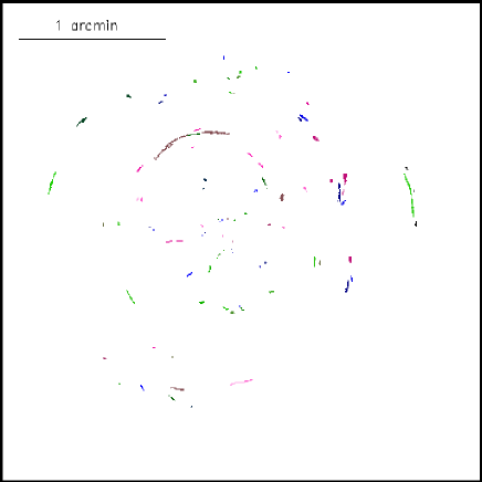
Figure 1: Data used in the mass reconstruction. There are 106 arcs in this image which are assigned to 30 different sources. Every arc has a flag associated to the putative source. Sources’ redshifts range from $z\approx 1$ to $z\approx 6$. The area in this plot is similar to the field of view of the original data and it covers $3.3\times 3.3$ arcmin².

The data used in this paper is described in detail in B2004. Here we only briefly summarize its main characteristics. The original ACS image of A1689 was obtained after integration of 20 orbits with the Hubble space telescope in 4 bands (G,R,I and Z). The final published image covers a field of view of $3.3\times 3.3$ arcmin² with a pixel size of $0.05\times 0.05$ arcsec². The catalog with the coordinates and redshifts of the contains the positions and redshifts of 106 arcs, 7 of which have been spectroscopically identified in previous works (Fort et al. 1997, Frye et al. 2002). The bulk of the redshifts were estimated using the Bayesian software BPZ (Benítez 2000). In addition to the five bands mentioned above, the ACS observations were complemented with U-band observations obtained with the DuPont telescope at Las Campanas Observatory and J,H,K data at La Silla with the NTT telescope. With these bands, the final photometric redshifts are typically uncertain by 15-20 %. The 106 arcs are associated with 30 systems or sources with redshifts in the range $1<z<6$.. The positions in the catalog correspond to the center of the arc. We only use these central positions to identify the arcs. Then we carefully select all the pixels in each arc to build the final strong lensing data set. We go through all the tabulated positions and select the pixels belonging to the specified arc by eye. We only select the pixels which are clearly connected with the arc. In the cases where the arc is too faint, a smoothed version of the data is used to enhance the signal to noise ratio. Eye selection is superior to algorithm selection in our case since software can not be trusted to separate the faintest arcs from the background. After all the positions in the arcs have been selected we repixelize the data in an area of $5\times 5$ arcmin² using $512\times 512$ pixels. Under this pixelization, the total number of pixels in our data set containing part of an arc is $N_{\theta}=601$. The resulting data set is show in figure 1. These are the 601 $\theta$ positions which are used to invert the lens. The results are described in the next section.

4 The recovered mass distribution of A1689

In this section we present the results of our analysis when applying the method of section 2 on the data from section 3. We show the results of 1000 minimizations, where the initial mass distribution and source redshifts are randomly varied. The maximum number of mass-cells is approximately 600.

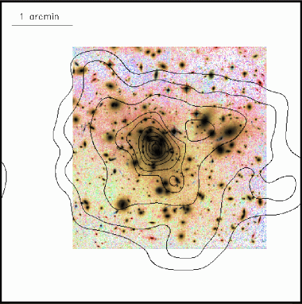
Figure 2: Mean recovered mass (contours) compared with true ACS image. The mass is the average of 1000 minimizations of the lens equation where at each minimization we change the grid, the initial conditions, $X_{o}$ and the redshifts of the sources. Contours go from $0.1$ to $0.97$ times the maximum mass density in intervals of $0.1$ ($0.097$ last interval). Total mass in the field of view is about $5.2\times 10^{14}h^{-1}M_{\odot}$. The field of view in this plot and the others is $5\times 5$ arcmin² unless otherwise noted.

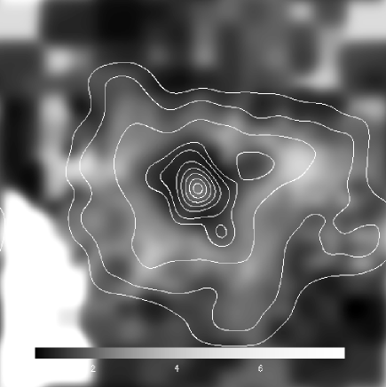
Figure 3: This grey scale map shows the signal to noise ratio (SNR) of the recovered mass which is obtained by dividing the mean recovered mass by the dispersion of the 1000 recovered maps. For clarity, the areas with SNR$>$8 have been saturated (white color). Note the low SNR at about 20” from the center of mass. The contours show the mean recovered mass of figure 2 The field of view is $5\times 5$ arcmin².

The result of this minimization process is shown in figure 2 where we compare the average of the 1000 recovered solutions with the ACS optical image of A1689. Keeping in mind that no information about the luminosity is used, the first obvious conclusion from this plot is the existing correlation between the luminous and the dark matter. The peak of the mass distribution falls very close to the central cD galaxy. There is also a clear correlation between the position of the subgroup to the right and a secondary peak in the mass distribution. The small subgroup at $\approx 30^{\prime\prime}$ to the south of the cD seems to be sitting close to the top of other over-density.

The substructure within 1 arcmin of the center of the cluster suggests that the cluster is not fully relaxed. Another possibility is that some of the substructure arises from projection rather than from substructure within the main cluster. However, the existing correlation between the recovered mass and the galaxies suggest that the substructure may be really present in the cluster. Another interesting feature is that the reconstructed mass seems to be insensitive to the external structure of A1689. There seems to be no significant structure beyond 2 arcmins from the central cD. This can be explained if the mass distribution beyond this radius can be approximated by a spherical distribution. In this case Gauss’ theorem implies that the strong lensing data should be independent of the unknown outer mass distribution.

Looking at the dispersion of the 1000 minimizations tells us something about the reliability of our recovered mass profile. An estimate of the dispersion of these solutions can be seen in figure 3 where we plot the signal to noise ratio, or SNR, which is defined as the ratio of the mean recovered map divided by the standard deviation map of the solutions. The first thing we should notice is that around 20”, the SNR drops below 3. In other words, the mass estimate in this region can not be trusted as well as in other regions. A similar behaviour can be observed at large radius as discussed above and may imply a degeneracy set by the limitations of the data we are using. The insensitivity of the data to the outer regions of the mass distribution is suggested also when we look at the average 1D profile. The 1D density profile is defined as the average profile at a given distance from the center normalized by the critical density, defined as;

$$\Sigma_{crit}=\frac{c^{2}}{4\pi G}\frac{D_{s}}{D_{d}D_{ds}}=4.29\times 10^{15}\frac{hM_{\odot}}{Mpc^{2}}$$ (9)

In the previous expression, we have assumed that $\Sigma_{crit}$ is defined at the mean redshift of the sources, that is, $z=3$ (B2004). Note that the units of $\Sigma_{crit}$ are $hM_{\odot}/Mpc^{2}$. These are the same as the recovered $\Sigma$ which is defined as;

$$\Sigma=\frac{Mass}{pixel}=\frac{h^{-1}M_{\odot}}{(h^{-1}Mpc)^{2}}=\frac{hM_{\odot}}{Mpc^{2}}$$ (10)

The recovered 1D profile is shown in figure 4. Also shown is the dispersion of the 1000 recovered profiles. The dotted-dashed line shows the best fitting NFW profile (Navarro et al. 1995) found by B2004 using the same data. By comparing the reconstructed profile with an NFW profile we can confirm the excess found in B2004. This excess may also be well described by an NFW profile. We will discuss this point later but here we anticipate that the data is more likely to be compatible with an NFW profile plus an excess (thick solid line). However, it is clear from figure 4 that our reconstructed profiles differ significantly from an NFW profile at large radii thus suggesting a possible bias in our results here. This possibility will be explored in more detail later.

Figure 4: The plot shows the mean value (squares) and the $99\%$ confidence region of the 1D profiles for the 1000 minimizations in case $i)$. The dot-dashed line is the best fitting NFW profile found in B2004. The density has been rescaled by the critical density, $\Sigma_{crit}$. The thick solid line is a very similar NFW profile plus an excess given by 3 NFW subhaloes around the main halo. See text for details.

When we look at the normalized 1D profile (figure 4), we find another striking feature which also suggests possible bias in our results, this time in the very central region. As opposed to previous results based on the same data (B2004), the central density deviates from a NFW profile and even shows a dip at distances around 20 arcsec from the central peak. The same dip can be observed if we look at the map of the signal to noise ratio, or SNR (see figure 3). This may be an indication that our algorithm is more sensitive to tangential than radial arcs. The radial images contain more information about the matter distribution in the very center of the cluster than the tangential ones. This could be explained because we are minimizing the residual of the lens equation. The residual is basically dominated by the tangential arcs since they have more pixels than the radial arcs and therefore contribute more to the residual. Again, this possible bias will be explored later.

Finally, an interesting conclusion from figure 4 is that using a non-parametric algorithm does not mean necessarily that the solution cannot be well constrained within the error bars. In fact, these error bars are comparable to the ones obtained with parametric methods.

5 Predicted positions of the sources.

The solution found in the previous section also gives us the original position of the sources. Let us recall that in our algorithm we assume that the sources are point-like and they are described by just two numbers, namely the $x$ and $y$ coordinates at the center. For each of the 1000 minimizations we obtain an estimate of the $(x,y)$ position of each source. The result is plotted in figure 5. The recovered sources fall in a small area of $\approx 1\times 1$ arcmin². Some sources seem to fall on top of others. Given the uncertainties in the photometric redshifts, it could happen that some of the sources are at the same redshift. This, together with the fact that they appear in the same area in the sky, make us think that some of these sources may be the same. We should note however that previous work has identified a systematic problem when minimizing the lens equation in the source plane, namely the fact that the minimization is biased toward higher masses for the lens and with the sources being in a more compact region. If we are indeed affected by this, this would explain why the sources seem to fall in such a compact region. This possible systematic effect will be also studied later.

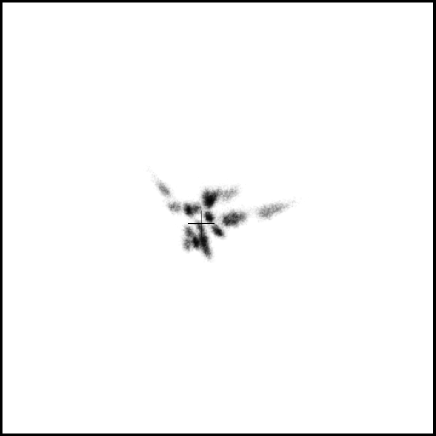
Figure 5: Zoomed version of the recovered $\beta$ positions after 1000 minimizations. The field of view is $3.3\times 3.3$ arcmin. The cross marks the position of the cD galaxy. Note how the small area of the source plane relative to the image plane and implies a high magnification of the background galaxies with a mean value of $\sim 8$.

6 Critical curves

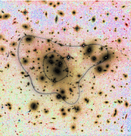
Figure 6: Critical curves for the mean recovered mass in figure 2. The field of view is the same as the original image (3.3 arcmin). Note the clear formation of a radial critical curve whose size relative to the tangential critical curve requires a shallow central mass profile.

It is interesting to look at the critical curves of our reconstructed mass. These curves are defined as the regions where the magnification diverges. Normally one expects to see two kind of curves, the tangential critical curve and the radial critical curve. The first one is normally associated with the Einstein radius and is where the big radial arcs tend to appear.

The radial critical curve defines the region where two multiple images merge or split in the radial direction. This curve is very interesting because it is sensitive to the particular profile of the inner region of the cluster. If we change the total mass, the concentration parameter and the characteristic scale, $r_{s}$, such that the tangential critical curve does not change much (i.e, we do not change the mass embedded within the giant tangential arcs) then we observe that smaller $r_{s}$’s produce smaller radial critical curves. In other words, the ratio between the tangential and the radial critical curves tells us something about the steepness of the profile between the radii of the giant arcs and the center. A steep profile will produce a small relatively small radial critical curve, for a fixed tangential critical curve. A relatively large radial critical curve, is generated by a flatter profile near the center of the cluster. Note that for profiles steeper than the isothermal case, the radial critical curve is reduced to a point at the position of the lens.

Previous analysis of A1689 based on the same data (B2004) found a relatively large radial critical curve extending up to 20” from the center of the cluster. NFW profiles are compatible with these large radial critical curves only if the halo characteristic radius, $r_{s}$, is relatively large. B2004 found best fitting values of $r_{s}=310h^{-1}$ kpc and concentration parameter $C_{N}=8.2$ (with $C_{N}=R_{virial}/r_{s}$). An NFW profile like this one reproduces well the derived critical curves in B2004.

The critical curves of our mean recovered model (see figure 2) are shown in figure 6. By comparing with the critical curves in B2004 we see that the inner curve (radial critical curve) is similar (or even larger in some areas) than the one obtained in B2004. This fact suggests that the characteristic scale, $r_{s}$, must be indeed large, of the order of 300 $h^{-1}$ kpc or more. Also from the same plot, our critical curves show a smoother behavior than previous analysis (B2004), which may suggest that we are not very sensitive to small details in the mass distribution. More specifically, the differences between our recovered critical curves and the ones found in B2004 are bigger in the case of the radial critical curve which is more sensitive to the details in the central part of the cluster. A higher resolution is expected in the center for the modeling of B2004 because of the mases of the tight clump of luminous cluster galaxies found there are included in the model as part of the cluster sequence component (B2004). This level of detail which is not easy to reproduce in detail with our fully non-parametric model, which would require more constraints in the center for a more detailed fit here, hence our results in the center $r<20^{\prime\prime}$ should probably be regarded as a somewhat smoothed version of the central mass profile. This very last point may be connected with the drop interior to the critical curve (around 20” from the center) in the mass density profile (see figure 4). This feature in the profile could be due to a degeneracy among the masses in the cells in the very central region of the cluster and could be easily explained by the argument used above that our algorithm is less sensitive to the radial than to the tangential arcs. The features in the profile may be real or due to a systematic bias in our algorithm. Answering this question is the purpose of the next sections.

7 Error analysis and possible systematics

The results in the previous section offer some answers about the mass distribution in A1689 but also raise some serious questions about the reliability of our results. A visual comparison with the results of B2004 indicates some disagreement between our mass distribution and theirs. Our recovered mass distribution shows substructure within the central 200 $h^{-}1$ kpc ($1.5$ arcmin) with dips and peaks around the central peak. The overall mass distribution is similar in shape to that of B2004, but with more pronounced substructure. The difference can be partially explained by the fact that parametric methods implicitly assume a smooth distribution for the main dark matter component with no dips while we do not. The second possibility is that the dips are an artifact coming from degeneracies of the modelling procedure. As shown in paper I, one may expect a variety of models to be consistent with the data. Some of these models may show degeneracies between neighboring cells at small scales if the result is not sensitive to these small scales, although in general is not possible to predict where the degeneracies will appear. One expects that the range of valid models reduces as the number of arcs increases. This means that each case has to be studied separately. This possibility will be explored further in the next section.

In this section we focus on another source of systematics. In section 4 we included in our analysis the numerical uncertainties in our algorithm. They were the uncertainty in the knowledge of the redshift of the sources and the uncertainty in the shape of the sources. The uncertainty in the redshift was included by assigning different redshifts to the sources at each minimization (Gaussian distribution), while the uncertainty in the shape of the sources was included by minimizing many times, each one with a different initial condition, $X_{o}$.

In section 4 we also changed the grid at each iteration using our dynamical adaptive grid which constructs the new grid based on the previous solution. For doing that we had to fix one parameter of the algorithm, the total number of cells, $N_{c}$. The algorithm needs another parameter to be defined, namely the minimum residual we want to achieve, $\epsilon$. The algorithm stops when $R^{2}<\epsilon$, where $\epsilon$ can be defined by the size of the sources and their number. In sections 2 and 4 we gave some intuitive motivation on how to choose $\epsilon$ and $N_{c}$ respectively. In this section we address the issue of how sensitive the results are to these two parameters.

We consider three different scenarios or cases.
$\bullet$ Case $i)$, the minimization is performed with a number of cells $N_{c}\approx 600$ and $\epsilon=2\times 10^{-11}$. This is the case used to present the results in section 4.
$\bullet$ Case $ii)$, as in case $i)$ but we reduce the number of cells to $N_{c}\approx 300$.
$\bullet$ Case $iii)$, as in case $i)$ but we reduce the size of the sources to $\epsilon=5\times 10^{-12}$

Figure 7: Recovered 1D profile with error bars (at 99 % level). The dot-dashed line is the best NFW profile found in B2004. This is case for ii) (300 cells, $2E-11$).

Case $i)$ was already studied in the previous sections and is used here for comparison. For each of the cases $ii)$ and $iii)$ , we run another 1000 minimizations changing the starting point, $X_{o}$, the redshifts and the grid as we did in case $i)$ (section 4).

In case $ii)$, by reducing the number of cells we reduce the number of possible solutions, i.e we reduce the uncertainty in the solution. We also degrade the resolution since we have to fill the same space ($5\times 5$ arcmin²) with half the number of cells. After averaging 1000 minimizations, the recovered mass distribution looks similar to the one found in case $i)$ with the main difference being in the outer areas were case $ii)$ shows an even larger deficit in mass when compared to the NFW profile. The critical curves^⋆ also look very similar to the ones found in case $i)$ but showing a slightly larger radial critical curve which suggests a higher concentration of mass near the center of the cluster. The average of the 1D profiles together with its $99\%$ error bars can be seen in figure 7. The plot clearly demonstrates the departure from the NFW profile at large radii. It also shows the reduction in the dispersion of the solutions as well as a lack of a dip at 20”. The same effect can be seen when we look at the predicted position of the sources (figure 8). Contrary to what happened in case $i)$ (see figure 5), the predicted positions of the sources in case $ii)$ do not suggest a smaller number of sources. A closer look reveals that in case $ii)$ the smaller number of cells produces a sequence of grids with very small differences between them. In other words, in case $ii)$ we are in a situation in which the grid has been practically fixed from iteration 1. This fact contributes crucially to the reduction in the range of solutions (masses and $\beta$ positions).

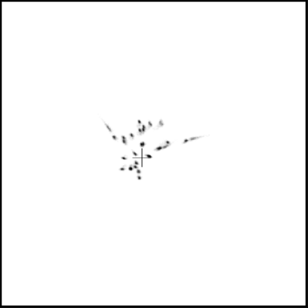
Figure 8: Zoomed version of the recovered $\beta$ positions after 1000 minimizations for case $ii)$. Field of view is $3.3\times 3.3$ arcmin².

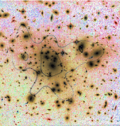
Figure 9: Critical curves for the mean recovered mass in the case $iii)$. The field of view is (3.3 arcmin)²

Case $iii)$ is interesting to explore because it forces the algorithm to find a solution closer to the unphysical point source solution. The total dispersion in the source plane has now been reduced by a factor 4. The solutions achieve this by adding more substructure to the mass distribution and when $\epsilon$ is made small enough, the $\beta$ positions are also shifted toward the position of the center of mass. This effect is well known and it was studied in paper I. In our particular case, the mean mass distribution of the 1000 solutions looks again similar^⋆ to the one found in case $i)$ but showing more substructure. The average 1D profile^⋆ is also similar to the one in figure 5. Here we present only the critical curves in figure 9 were the effect of the extra substructure can be appreciated.
The residual, $R$ or $\epsilon$, has the physical meaning of being the variance or size of the sources. Setting a very small $\epsilon$ produces a biased mass distribution which focuses the arcs into very small sources or point sources. The point source solution achieving this is normally unphysical as it was shown in paper I. On the contrary, choosing a large $\epsilon$ will stop the minimization early, resulting in a short sighted cluster, meaning the solution cannot focus the arcs properly. This short sighted cluster solution is normally a smoother, lower-mass version of the real solution.

8 Testing the results with simulations

The previous section has two possible interpretations. On the pessimistic side, we raised concerns about the reliability of our results since we show how the results change depending on our choice of number of cells and the stopping point of the minimization. On the other hand, the positive interpretation is that the change in the results is not dramatic and our conclusions seem to be relatively insensitive to big changes in the minimization process.

Although the last section gave us an idea about the dispersion in the solution, it did not address the issue of whether or not the recovered solution is biased. The problem in answering this question is of course that we do not know what the real mass distribution is, thus there is nothing to compare our results with. The aim of this section is to rectify this by using a simulated data set which mimics the main features of the real data. With a simulation we can easily check aspects like how sensitive the data is to the mass distribution in the very center or in the area beyond the tangential arcs. Our simulated cluster is a simplified version of the recovered mass distribution, made up of a superposition of NFW profiles. Since the recovered solution has a mass deficit in the outer parts, the simulated cluster has a larger total mass, but is chosen so that it resembles well the mass distribution within the giant arcs.

We use a total mass of $M_{T}=0.68\times 10^{15}h^{-1}M_{\odot}$ in the field of view ($5\times 5$ arcmin²). For simplicity, our simulated cluster is made of only four NFW halos. The main halo is assigned a mass of $M_{1}=0.53\times 10^{15}h^{-1}M_{\odot}$ and placed at the maximum of the averaged recovered mass in section 4. The second halo is given a mass of $M_{2}=0.07\times 10^{15}h^{-1}M_{\odot}$ and centred in the northeastern subgroup. The third halo with $M_{3}=0.03\times 10^{15}h^{-1}M_{\odot}$ is centered to the south-east of the main group, and finally the fourth halo with $M_{2}=0.05\times 10^{15}h^{-1}M_{\odot}$ is placed to the north-west of the main halo (see figure 10). This simulated cluster resembles the reconstructed mass profile found in section 4 but with the difference that it has a sharp cusp in the center (plus 3 off-peak sharp cusps) and the tails of the distribution do not fall off as quickly as in the recovered mass distribution. We have also verified that the model roughly reproduces the recovered critical curves^⋆. The 1D profile of this simulated cluster is shown in figure 4 (thick solid line) where it is compared with the reconstructed 1D profile and the best fitting NFW profile of B2004. The projected mass distribution is shown in figure 10. For the lensing simulation the cluster is located at the same redshift as A1689 ($z=0.18$).

The second ingredient of the simulation are the sources. We use 30 sources whose $\beta$ positions are taken as random within a box of $1\times 1$ arcmin around the center of the main halo. The sources are assumed to be circular with radii of a few kpc, and are placed at the redshifts published in B2004.

The final part of the simulation is to find the arcs corresponding to the previous configuration^⋆. For this we use a simple ray-tracing algorithm.

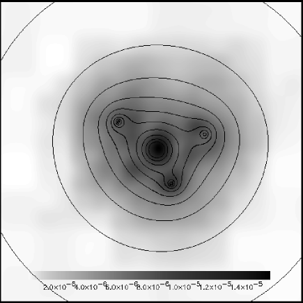
Figure 10: Recovered mass (grey scale) compared with the original simulated one (contours). The contours increase in steps of 0.5 times the maximum central density starting at 0.05 times the maximum. The units of the greyscale map are $10^{15}h^{-1}M_{\odot}/pixel$ and there are $512^{2}$ pixels in the image. The field of view is (5 arcmin)²

With this simulated data we follow a reconstruction process similar to the case $i)$ in the previous section. We run 1000 minimizations (but with 500 cells instead of 600 and with $\epsilon=2.0\times 10^{-11}$) and calculate the mean value and dispersion of the solutions.

Figure 11: The mean and error bars of the 1000 recovered profiles after changing the initial conditions, $X_{o}$, the redshifts and the grid at each minimization. The thick solid line is the original profile of the simulated cluster.

The average of the 1000 recovered masses is shown in figure 10 as a grey scale map and it is compared with the original mass distribution (contours). The position of the main halo is reconstructed with good accuracy. In the position of the secondary halos we reproduce an over-density although a spurious over-density also appears in the south-west of the main halo. The total recovered mass is $4\times 10^{15}h^{-1}M_{\odot}$, that is 40 % smaller than the original total mass. This deficit in mass is again concentrated in the outer areas, beyond the position of the giant arcs as can be seen from the recovered 1D profile (figure 11). The simulation confirms that the algorithm is insensitive to the mass distribution beyond the most distant arcs from the centre. Another interesting conclusion from figure 11 is that the algorithm also seems to have some problems finding the right mass in the central region. It over-predicts the central density and under-predicts the density in the area near the radial critical curve. It even suggests a fictitious dip in this area. When we repeat the same exercise but reducing the number of cells down to 300 (and keeping $\epsilon=2\times 10^{-11}$, we observe a similar behaviour to the one described in section 7^⋆. The recovered 1D profile does not show a dip at 20” and the profile falls faster at radii larger than 60”. Between 20” and 60”, the 1D profile over-predicts the real one by about 20 % in the case with 300 cells.

An interesting lesson can be learned when we combine both results. The recovered mass distribution interior to the radial critical curve is closer to the real one when we use a smaller number of cells (300) but between the radial and the tangential critical curves, the recovered mass profile is better when we increase the number of cells (500-600). Unsurprisingly, we are also able to conclude that we definitely recover a biased mass distribution beyond 70”or 80” from the centre.

Regarding the location of the sources, the recovered $\beta$ positions deviate from the true position by between 0” and 5” (see figure 12). Reducing the number of cells from 500 to 300 does not show any appreciable improvement in this situation and the recovered $\beta$ positions look almost indistinguishable from figure 12. This is to be contrasted by case $ii)$ in section 7. However, as opposed to that case, reducing the number of cells to 300 in the simulated data does not here produce a sequence of almost identical grids. This suggest that the recovered positions of case $ii)$ in section 7 (see figure 8) are more the product of fixing the grid than being the real position of the sources.

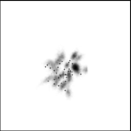
Figure 12: Reconstructed positions of the sources (grey scale) for 1000 minimizations. The true position of the sources is marked with small crosses. The big cross is the position of the main halo. The field of view is a zoomed version ($2\times 2$ arcmin) of the original 5 arcmin field of view.

9 Conclusions

Using a non-parametric algorithm (SLAP) we reconstruct the mass distribution of A1689 based on strong lensing data containing the 106 multiply lensed images identified by B2004. The reconstructed mass agrees well with previous estimations based on parametric algorithms (B2004). Our non parametric approach is an essential complement to the more model dependent methods and also allows us to understand better the uncertainties and potential ambiguities involved in using strong lensing data for generating surface mass distributions. In particular, we find that our recovered mass is biased toward smaller values beyond the most external tangential arcs and there is some evidence for degeneracy problems in the very central region. However, we also conclude that the total mass can be well constrained within 70” from the center of the cluster. The total projected mass within 70” from the center is found to be $0.25\times 10^{15}h^{-1}M_{\odot}$. The simulated work suggest that the estimated profile between 20” and 70” is reliable.
It also shows how the degeneracy in the central region can be reduced by taking a smaller number of cells which naturally decreases the degrees of freedom. This is done at the expense of a bias in the outer regions which is increased when the number of cells is low. Testing the algorithm with simulations which mimic the real data and the average estimated mass we found that the best results can be obtained combining a minimization with a relatively large number of cells ($N_{c}\approx 500$) with a minimization with a smaller number of cells ($N_{c}\approx 300$). Combining these results we find that the mass recovered in a non-parametric way is compatible with a NFW profile plus an excess associated to substructure around the central overdensity.

Our modeling indicates that the central region of the cluster is either affected by projection along the line of sight or is not yet fully relaxed as significant local density perturbations are found in our reconstruction. Evidence of ongoing merging has been also reported from an analysis of recent X-ray data (Andersson & Madejski 2004). The mass derived from the X-ray profile is about two times smaller than the one derived here when the cluster is assumed to be in a relaxed state (Andersson & Madejski 2004). If one believes the lensing results, it means the assumption of hydrostatic equilibrium used to derive the mass from X-rays may be hard to justify in detail (Xue & Wu, 2002).
Previous analysis of A1689 using different lensing techniques support this hypothesis as they tend to agree in the mass (Tyson & Fischer 1995, Taylor et al. 1998, Dye et al. 2001). Our integrated mass estimate agrees well with these previous analises^⋆.

In the bibliography one can find numerous studies of how masses derived from X-rays, optical and lensing compare (Miralda-Escudé & Babul 1995, Allen 1998, Wu et al. 1998, Wu 2000, Cypriano et al. 2004). Systematically, a discrepancy of about 2-4 is found in the central regions of some clusters, specially in the ones with evidence of being in a non-relaxed state (Allen 1998). A combination of the gravitational potential in the central region derived from strong lensing observations with high resolution X-ray data will allow exciting studies focusing on the dynamical state of the gas in these regions. Also interesting is to combine the strong lensing results in the central region with weak lensing information which allows to extend the analysis up to Mpc scales (Broadhurst et al. 2004b).

10 Acknowledgments

This work was supported by NSF CAREER grant AST-0134999, NASA grant NAG5-11099, the David and Lucile Packard Foundation and the Cottrell Foundation. The authors would like to thank Elizabeth E. Brait and E.Hayashi for useful discussions.

References

- [1] Abdelsalam H.M., Saha P. & Williams, L.L.R., 1998, MNRAS, 294, 734.
- [2] Abdelsalam H.M, Saha P. & Williams, L.L.R., 1998, AJ, 116, 1541.
- [3] Allen S.W., 1998, MNRAS, 296, 392.
- [4] Andersson K.E., Madejski G.M., 2004, ApJ, 607, 190.
- [5] Benítez N. 2000, ApJ, 536, 571.
- [6] Bartelmann M., Narayan R., Seitz S. Schneider P., 1996, ApJ, 464, L115. 2004, PhRvL, 92, 1301.
- [7] Broadhurst T.J., Taylor A.N., Peacock J.A., 1995, ApJ, 438, 49.
- [8] Broadhurst T., Benítez N., Coe D., Sharon K., Zekser K., White R., Ford H., Bouwens R., 2004a, Astrophysical Journal, in-press. preprint astro-ph/0409132. B2004.
- [9] Broadhurst T., Takada M., Umetsu K., Kong X., Arimoto N., Chiba M., Futamase T., 2004b, in preparation.
- [10] Cypriano E.S., Sodré L Jr., Kneib J.P., Campusano L.E., 2004, ApJ, 613, 95.
- [11] Diego J.M., Protopapas P., Sandvik H.B, Tegmark M. 2004, MNRAS submitted. preprint astro-ph/0408418. Paper I
- [12] Dye S., Taylor A.N., Thommes E.M., Meienheimer K., Wolf C., Peacock J.A.,
- [13] Fort B., Mellier Y., Dantel-Fort M., 1997, A&A, 321, 353.
- [14] Frye B., Broadhurst T. Benítez N. 2002, ApJ, 568, 558. 1998, ApJ, 503, 531.
- [15] Kneib J.-P., Mellier Y., Fort B., Mathez G., 1993,A&A, 273, 367.
- [16] Kneib J.-P., Mellier Y., Pello R., Miralda-Escudé J., Le Borgne J.-F.,Boehringer H., & Picat J.-P. 1995, A&A, 303, 27.
- [17] Kneib J.-P., Ellis R.S., Smail I.R., Couch W., & Sharples R. 1996, ApJ, 471, 643.
- [18] Kochanek C.S. & Blandford R.D., 1991, ApJ, 375, 492.
- [19] Miralda-Escudé J., & Babul A. 1995, ApJ, 449, 18.
- [20] Navarro J.F., Frenk C.S., White S.D.M., 1995, MNRAS, 275, 720.
- [21] Press W.H., Teukolsky S.A., Vetterling W.T., Flannery B.P., 1997, Numerical Recipes in Fortran 77. Cambrdige University Press.
- [22] Saha, P., Williams, L.L.R., 1997, MNRAS, 292, 148.
- [23] Saha P. 2000, AJ, 120, 1654.
- [24] Sand D.J., Treu T. Ellis R.S. 2002, ApJ, 574, 129.
- [25] Schneider P., 1995, A&A…302..639S.
- [26] Schneider P., & Seitz C. 1995, A&A, 294, 411.
- [27] Taylor A.N., Dye S., Broadhurst T.J., Benitez N., van Kampen E. 1998, ApJ, 501, 539.
- [28] Trotter C.S., Winn J.N., Hewitt J. N., 2000, ApJ, 535, 671.
- [29] Tyson J.A., Fischer P., 1995, ApJ, 446, L55.
- [30] Tyson J.A., Kochanski G.P., Dell’Antonio I., 1998, ApJL, 498, 107.
- [31] Wu X.-P., & Fang L.-Z. 1997, ApJ, 483, 62.
- [32] Wu X-P., Chiueh T., Fang L-Z., Xue Y-J., 1998, MNRAS, 301, 861.
- [33] Wu X-P., 2000, MNRAS, 316, 299.
- [34] Yamamoto K., Kadoya Y., Murata T., Futamase T., 2001, Progress of Theoretical Physics, 106, 917.
- [35] Xue S-J., Wu X-P., 2002, ApJ, 576, 152.